Abstract

To efficiently implement many-qubit gates for use in quantum simulations on quantum computers we develop and present methods reexpressing $\exp[-i(H_{1}+H_{2}+\dots)\Delta t]$ as a product of factors $\exp[-iH_{1}\Delta t]$, $\exp[-iH_{2}\Delta t]$, $\dots$ which is accurate to 3rd or 4th order in $\Delta t$. The methods we derive are an extended form of symplectic method and can also be used for the integration of classical Hamiltonians on classical computers. We derive both integral and irrational methods, and find the most efficient methods in both cases.

1 Introduction

Quantum computers have generated much interest recently, largely due to the result by Shor [1] that they can factor integers in polynomial time.

In a quantum computer the analog of a logical bit is the qubit. The canonical example of a qubit is a quantum spin. A quantum spin consists of two states, so a set of $n$ spins gives the quantum computer a $2^{n}$-dimensional Hilbert space.

To perform a calculation, one initializes the qubits, and then applies unitary logical gates to the qubits. Unitary logical gates are realised in different fashions depending on the quantum computer hardware, but they are all represented mathematically by a Hamiltonian acting on the quantum state of the qubits. In a typical quantum computer, technology restricts the Hamiltonian to act on a small number of qubits at a time, maybe two or three. A calculation is then built up of two- or three-qubit Hamiltonians, or gates, acting sequentially on the qubits.

An important and difficult to realise requirement is that the qubits maintain their coherence throughout an entire calculation. Maintaining coherence in quantum computers is a problem which has led to the development of error correcting codes (see [2] and included references). These codes are possible due to the fact that one does not need to know the state of a qubit in order to tell whether an error has occurred. With some ingenuity, it is possible to determine what kinds of errors have occurred during the course of a calculation and to correct the errors as the calculation proceeds. Simple error correction codes have already been shown to work on small numbers of qubits [3].

Effort has also been put into developing algorithms which make use of the quantum computer’s power. Shor’s algorithm showed that quantum computers are more powerful than classical computers, since integers cannot be factored in polynomial time on a classical computer, whereas they can on a quantum computer. Grover has also devised a method for searching a database in time proportional to the square root of the number of items involved in the search [4].

In addition to research into effective algorithms for use on quantum computers, simulations of quantum systems have also been shown to be possible in polynomial time [5]. Indeed, this was the first area for which it was proposed that quantum computers could fundamentally be more powerful (i.e. much faster) than classical computers [6].

This paper focuses on a problem which concerns simulational issues in quantum computation. Essentially, we have developed methods for reexpressing $\exp[-i(H_{1}+H_{2}+\dots)\Delta t]$ as a product of factors $\exp[-iH_{1}\Delta t]$, $\exp[-iH_{2}\Delta t]$, $\dots$ which is accurate to 3rd or 4th order in $\Delta t$, as mentioned in the abstract.

A simulation on a quantum computer consists of applying an operator $\exp(-iHt)$ on a set of qubits, where $H$, the Hamiltonian of the system of interest is suitably encoded (and discretized) to act on the set of qubits. For many body systems, $H$ is a sum of terms. For instance, in a one-dimensional Ising spin model, the Hamiltonian is

$$H=\sum_{n=1}^{N}\vec{\sigma}_{n}\cdot\vec{\sigma}_{n+1}$$ (1)

where $N$ is the number of spins. Another example is the Hubbard model Hamiltonian, used in the study of high-$T_{c}$ superconductivity, which can be written [7] as the sum

$$H=\sum_{i=1}^{m}V_{0}n_{i\uparrow}n_{i\downarrow}+\sum_{\langle i,j\rangle\sigma}t_{0}c_{i\sigma}^{*}c_{j\sigma}$$ (2)

where $V_{0}$ is the strength of the potential, and $n_{i\sigma}$ is the operator for the number of fermions of spin $\sigma$ at site $i$. In the second (kinetic energy) term, the sum $\langle i,j\rangle$ indicates all neighboring pairs of sites, $t_{0}$ is the strength of the “hopping”, and $c_{i\sigma}$, $c_{i\sigma}^{*}$ are annihilation and creation operators, respectively, of a fermion at site $i$ and spin $\sigma$.

These models give examples in which a large simulation on a classical computer is impossible due to the exponential increase in the size of the Hilbert space of the quantum system with the number of lattice sites. A many-particle system can sometimes be simulated with fewer qubits in first-quantized form [7], but in either case the Hamiltonian $H$ is a sum of terms, so our methods are equally applicable to both cases.

If the quantum computer cannot act on all spins at once, as is the case for quantum gate arrays [8], it becomes necessary to find ways of approximating the application of the above Hamiltonians with few-qubit gates. To second order, for instance, we find that

$$\left(e^{-iH_{1}\Delta t}e^{-iH_{2}\Delta t}\ldots e^{-iH_{N}\Delta t}\right)\left(e^{-iH_{N}\Delta t}\ldots e^{-iH_{2}\Delta t}e^{-iH_{1}\Delta t}\right)=e^{-i2(H_{1}+H_{2}+\ldots H_{N})\Delta t+{\cal O}\left[\left(\Delta t\right)^{3}\right]}$$ (3)

where $H_{n}$ are two-qubit gates (e.g. $\sigma_{n}\cdot\sigma_{n+1}$).

Below, we analyze the problem of deriving higher order methods of this type, and find a set of equations which, once solved, give $3$rd and $4$th order methods analogous to the above second-order method. We solve and present the formulae for $3$rd and $4$th order methods as well as developing methods for approximating expressions involving commutators, $\exp([A,B])$. Since there is a large set of solutions to our equations, we spend some effort trying to isolate and present only the most efficient methods.

After presenting our methods, we then provide results from a simple application to give the reader confidence that our methods are correct.

This kind of method has been investigated elsewhere, for different reasons, in the context of Hamiltonian systems under the name ‘symplectic’ method. In the section on symplectic methods, we comment on what we have done differently from other investigations of symplectic methods, and why our methods are applicable to more general problems. We then present a summary of our results in the conclusions section.

We also provide appendices with useful expressions used in the derivation of our results, and some proofs of statements in the text.

2 Mathematical Analysis and Equations

We want to express $\exp\left(\sum_{n=1}^{N}A_{n}\right)$ as a product of individual $\exp\left(A_{n}\right)$’s. In order to do this, we use the Campbell-Baker-Hausdorff formula. The Campbell-Baker-Hausdorff formula to 5th order is

$$\exp\left(aA_{1}\right)\exp\left(aA_{2}\right)=\exp\left[a\left(A_{1}+A_{2}\right)+\frac{1}{2}a^{2}A_{12}+\frac{1}{12}a^{3}\left(A_{112}+A_{221}\right)+\frac{1}{24}a^{4}A_{1221}\right.$$

$$\left.\mbox{}-\frac{1}{720}a^{5}\left(A_{11112}-2A_{21112}-6A_{11221}-6A_{22112}-2A_{12221}+A_{22221}\right)+{\cal O}\left(a^{6}\right)\right]$$ (4)

where

$$A_{kl\ldots mn}\equiv[A_{k},[A_{l},\ldots[A_{m},A_{n}]\ldots]]$$ (5)

To find combinations of operators $\exp{A_{i}}$ which approximate $\exp\left(\sum_{n=1}^{N}A_{n}\right)$ to some order it is first necessary to choose a strategy for searching among the large number of possible combinations. First of all, we cannot search brute force since there are too many possible combinations, and, in any case, this would not give us a formula valid for all $N$. Therefore, we pick a fundamental ordering of the product of exponentials with parameters allowing for transposes of the entire product as well as raising all the exponentials in the fundamental unit to the same power.

By iterating the Campbell-Baker-Hausdorff formula, we can get an expression for the fundamental unit in terms of a single exponential

$$\left(e^{aA_{1}}e^{aA_{2}}\ldots e^{aA_{N}}\right)^{\alpha}=\exp\sum_{p=1}^{\infty}\alpha a^{p}B_{N}^{p}$$ (6)

which defines the $B_{N}^{p}$ in terms of the $A_{n}$. Here, $p$ is an exponent on $a$, and a label on the matrices $B_{N}^{p}$. We take $\alpha=\pm 1$.

Now combine a succession $i=1,\dots,I$ of fundamental units with parameters $a_{i}$ and $\alpha_{i}$. Again iterating Campbell-Baker-Hausdorff gives

$$\exp\left(\sum_{p=1}^{\infty}\alpha_{1}a_{1}^{p}B_{N}^{p}\right)\ldots\exp\left(\sum_{p=1}^{\infty}\alpha_{I}a_{I}^{p}B_{N}^{p}\right)=\exp\left(\sum_{X}\sigma_{I}^{X}B_{N}^{X}\right)$$ (7)

The $B_{N}^{X}$ are generated from the $B_{N}^{p}$ by commutation. $X$ represents a label ${pq\ldots rs}$ where

$$B_{N}^{pq\ldots rs}\equiv[B_{N}^{p},[B_{N}^{q},\ldots[B_{N}^{r},B_{N}^{s}]\ldots]]$$ (8)

$B_{N}^{pq\ldots rs}$ is of order $p+q+\ldots+r+s$. Up to 5th order we can take

$$X\in\left\{1;2;3,12;4,13,112;5,14,23,113,221,1112\right\}$$ (9)

These $B_{N}^{X}$ span the space of commutators of the $B_{N}^{p}$’s to 5th order and for $N\geq 2$ they are independent. Formulae for the $B_{2}^{X}$ in terms of $A_{1}$ and $A_{2}$ are given in Appendix A.2. The $\sigma_{I}^{X}$ are defined in terms of $\alpha_{i}$ and $a_{i}$ by Eq. (7). Here again, the $X$’s are labels.

After some calculation, the Campbell-Baker-Hausdorff formula, Eq. (4), then gives

$$\sigma_{I}^{p}=\sum_{i=1}^{I}\alpha_{i}{a_{i}}^{p}$$ (10)

for $p=1,\ldots,5$,

$$\sigma_{I}^{pq}=-\frac{1}{2}\sigma_{I}^{p}\sigma_{I}^{q}+\frac{1}{2}\sum_{i=1}^{I}{a_{i}}^{q-p}\left[\left(\sigma_{i}^{p}\right)^{2}-\left(\sigma_{i-1}^{p}\right)^{2}\right]$$ (11)

for $pq=12,13,14,23$,

$$\sigma_{I}^{ppq}=-\frac{1}{2}\sigma_{I}^{p}\sigma_{I}^{pq}-\frac{1}{6}\left(\sigma_{I}^{p}\right)^{2}\sigma_{I}^{q}+\frac{1}{6}\sum_{i=1}^{I}{a_{i}}^{q-p}\left[\left(\sigma_{i}^{p}\right)^{3}-\left(\sigma_{i-1}^{p}\right)^{3}\right]$$ (12)

for $ppq=112,113,221$ ,

$$\sigma_{I}^{1112}=-\frac{1}{2}\sigma_{I}^{1}\sigma_{I}^{112}-\frac{1}{3}\left(\sigma_{I}^{1}\right)^{2}\sigma_{I}^{12}-\frac{1}{24}\left(\sigma_{I}^{1}\right)^{3}\sigma_{I}^{2}+\frac{1}{24}\sum_{i=1}^{I}a_{i}\left[\left(\sigma_{i}^{1}\right)^{4}-\left(\sigma_{i-1}^{1}\right)^{4}\right]$$ (13)

For approximations to $\exp\left(\sum_{n=1}^{N}A_{n}\right)$, we require all $\sigma_{I}^{X}=0$ except for $\sigma_{I}^{1}$ which is the coefficient of $B_{N}^{1}=\sum_{n=1}^{N}A_{n}$, and which should be greater than zero.

An interesting feature of 3rd order methods is that they require inverses, i.e. they require backward time evolution during part of the method. This can be proved using Eq. (10) with $p=3$. It has no nontrivial solutions when the product $\alpha_{i}a_{i}$ is positive for all $i$. Therefore for 3rd order methods, $\alpha_{i}a_{i}$ must be negative for at least one $i$. From the left hand side of Eq. (6), we see that this means that there must be at least one inverse. Similarly, from Eqs. (10) with $p=3$ and $p=4$ it can be proved that 4th order methods must have at least two inverses.

In Appendix A.1, we also prove the fact that for integral solutions $\sigma_{I}^{1}$ must be a multiple of 2 for a 2nd order method, a multiple of 6 for a 3rd or 4th order method, and a multiple of 30 for a 5th order method. Our searches suggest that the constraints on $\sigma_{I}^{1}$ may actually be stronger; all 4th order methods that we have found have $\sigma_{I}^{1}$ a multiple of 12, and we have not been able to find any 5th order methods.

In Section 7, we will consider approximation to $\exp[A_{1},A_{2}]$ for which we require all $\sigma_{I}^{X}=0$ except for $\sigma_{I}^{2}$.

3 Numerical Method for Solution of the Equations

We solve our equations for both integer and irrational solutions, using different methods for each search.

Our method to solve Eqs. (10-12) for integers is to pick values of $\alpha_{i}$ and $a_{i}$ and see if they satisfy the equations. To do this we restrict the number of fundamental units by fixing $I$. We also restrict the range of the $a_{i}$’s.

We start with Eq. (10), since, in this equation, order with respect to $i$ does not matter. So, for a given set of values, we need to consider only one permutation, not all permutations of the values. This greatly reduces the size of the search.

Furthermore, we start by considering $p=1$ and $3$, since it is only the sign of $\alpha_{i}a_{i}$ that matters in these equations. This means we can consider only the sign of the combination $\alpha_{i}a_{i}$, and not the signs of $\alpha_{i}$ and $a_{i}$ individually. This reduces the search further. These equations are particularly restrictive for the case of few inverses.

After solving the $p=1$ and $3$ equations, we introduce separate signs for the $\alpha_{i}$’s and $a_{i}$’s and solve the equation with $p=2$, and $p=4$ for the 4th order case.

Finally, into the restricted set of solutions to Eq. (10) we introduce permutations of the $\alpha_{i}$’s and $a_{i}$’s with respect to the index $i$ and solve Eqs. (10-12).

We solved Eqs (10) and (11) analytically to find the unique shortest irrational 3rd order method. To find 4th order irrational methods, we made a symmetric ansatz and solved Eqs. (10-12) analytically to find the shortest symmetric irrational 4th order methods. We checked numerically, using the globally convergent technique prescribed in [10], that these are all the shortest irrational 4th order methods.

The methods are presented in Section (5).

4 Criteria for Selecting Among the Solutions

With our strategy for finding solutions to Eqs. (10-12) we find a larger number of solutions than we can easily present. We need to select solutions to present and we also want to present solutions which are in some sense optimal. To do this, we consider the form of the operator resulting from a given method

$$\prod_{j=1}^{I}\left(e^{-ia_{j}A_{1}\,\Delta t}\,e^{-ia_{j}A_{2}\,\Delta t}\ldots e^{-ia_{j}A_{N}\,\Delta t}\right)^{\alpha_{j}}=\exp\left[-i\sigma_{I}^{1}\sum_{n=1}^{N}A_{n}\,\Delta t+r(-i\,\Delta t)^{o+1}\right]$$ (14)

where $\Delta t\ll 1$ is a time step, $o$ is the order of the method, and

$$r=\sum_{X}\sigma_{I}^{X}B_{N}^{X}$$ (15)

where $X\in\{4,13,112\}$ for a 3rd order method and $X\in\{5,14,23,113,221,1112\}$ for a 4th order method.

$r$ is an error which takes values in the vector space of the commutators for which we do not have a metric. Therefore, we make the ad hoc choice of basis that is given in Appendix A.3. This allows us to replace $r$ by a single real scalar $R$ as is also described in Appendix A.3. The error from the method can then be taken to be

$$E=nR\,\Delta t^{o+1}$$ (16)

where $n$ is the number of times we apply the approximate method.

If the physical time we want to simulate is $T_{p}$, then

$$T_{p}=nD\Delta t$$ (17)

where $D\equiv\sigma_{I}^{1}$ is given by the method.

The computer time it takes for a given simulation can be written

$$T_{c}=nINt_{g}+nLNt_{s}$$ (18)

where $I$ is the number of fundamental units in the method and $N$ is the number of terms in a unit, $t_{g}$ is the time it takes to make the gate change,

$$L\equiv\sum_{i=1}^{I}|a_{i}|$$ (19)

so that $LN$ is the total time the gates are applied for in the method, and $t_{s}$ is the time each individual gate is applied for. The time an individual gate is applied for will be $t_{s}=b\,\Delta t$, where $b$ is a proportionality constant dictated by the actual couplings in the quantum computer hardware.

Using Eqs. (16) and (17), the computer time can be rewritten

$$T_{c}=\left\{\left(\frac{T_{p}^{o+1}}{E}\right)^{\frac{1}{o}}\left(\frac{I}{D}\right)\left(\frac{R}{D}\right)^{\frac{1}{o}}t_{g}+\frac{LbT_{p}}{D}\right\}N$$ (20)

There are two possible limits to this equation. If $\Delta t$ can be made very small (from the hardware point of view), then making the error small forces the computer time to be dominated by gate switching. In this case, we want the factor

$$Z=(I/D)(R/D)^{1/o}$$ (21)

to be small.

If there is a lower limit to $\Delta t=\epsilon$, and it is reached before the computer time is gate switching dominated, then the computer time may be dominated by gate application. In this second limit, we want $L/D$ small, and to minimize the error $E$, we want $(R/D)(\Delta t)^{o}$ small. In this limit, each gate can only be applied for an integral number of the minimum timestep $\epsilon$. Thus, to use an irrational method, one must approximate the method by an integral method containing large integers, and so with a large $D$. Because $\Delta t=\epsilon$ is fixed, the error $E$ goes like $R/D\propto D^{o}$, and thus is large for irrational methods. We thus do not consider irrational methods in this limit.

To summarize, we want methods with small $L/D$ and $R/D$.

5 3rd and 4th Order Formulae for $\exp\left(\sum_{n=1}^{N}A_{n}\right)$

From this analysis, we want to choose methods for which $Z$, or $L/D$ and $R/D$ are small. Below we list the methods and their properties. We use the notation

$$(\alpha a)$$ (22)

to represent

$$\left(e^{aA_{1}}e^{aA_{2}}\ldots e^{aA_{N}}\right)^{\alpha}$$ (23)

if $\alpha=1$, and

$$(\alpha a)^{T}$$ (24)

to represent

$$\left(e^{aA_{1}}e^{aA_{2}}\ldots e^{aA_{N}}\right)^{\alpha}$$ (25)

if $\alpha=-1$. So, for example, the 2nd order method

$$\left(e^{A_{1}}e^{A_{2}}\ldots e^{A_{N}}\right)\left(e^{A_{N}}\ldots e^{A_{2}}e^{A_{1}}\right)=\left(e^{A_{1}}e^{A_{2}}\ldots e^{A_{N}}\right)\left(e^{-A_{1}}e^{-A_{2}}\ldots e^{-A_{N}}\right)^{-1}$$ (26)

is represented by

$$(1)(1)^{T}$$ (27)

Note that the transpose of any method gives another equivalent method, as does permuting the entries in the fundamental unit.

For odd order methods, the residue has an odd number of brackets in the commutators. So, because the transpose of an individual bracket is minus that bracket,

$$\left(\mbox{odd order method}\right)\left(\mbox{same odd order method transpose}\right)$$ (28)

gives a method of one order higher. For example, we can make a 4th order method from a 3rd order method, or a 6th order method from a 5th order method.

5.1 Integer solutions

The 3rd order integer methods that we have selected using the criteria of Section 4 are given below.

	3rd Order Methods
${\cal Z}_{3}^{1}$	$(1)^{T}(1)(1)(1)(1)^{T}(-2)^{T}(1)(1)(1)$
${\cal Z}_{3}^{2}$	$(1)^{T}(4)(2)(-5)^{T}(2)^{T}(3)(2)(2)^{T}(1)$
${\cal Z}_{3}^{3}$	$(1)^{T}(2)(2)(-3)^{T}(1)^{T}(2)(1)^{T}$
${\cal Z}_{3}^{4}$	$(3)(-4)^{T}(1)(3)(2)^{T}(1)$
${\cal Z}_{3}^{5}$	$(5)^{T}(7)(12)(-13)^{T}(1)$

	$D$	$L$	$I$	$L/D$	$R/D$	$Z$
${\cal Z}_{3}^{1}$	6	10	9	1.67	0.2	0.9
${\cal Z}_{3}^{2}$	12	22	9	1.83	0.6	0.6
${\cal Z}_{3}^{3}$	6	12	7	2.00	0.4	0.9
${\cal Z}_{3}^{4}$	6	14	6	2.33	1.7	1.2
${\cal Z}_{3}^{5}$	12	38	5	3.17	98.8	1.9

And the 4th order integer methods are

	4th Order Methods
${\cal Z}_{4}^{1}$	$(1)^{T}(1)(1)^{T}(-2)(1)^{T}(1)^{T}(1)^{T}(1)^{T}(1)(1)^{T}(1)(1)(1)(1)(-2)^{T}(1)(1)^{T}(1)$
${\cal Z}_{4}^{2}$	$(1)^{T}(2)(1)^{T}(-3)^{T}(2)(2)(1)(2)^{T}(2)^{T}(-3)(2)^{T}(1)(1)(1)^{T}$
${\cal Z}_{4}^{3}$	$(1)^{T}(2)(3)^{T}(1)^{T}(-4)(3)^{T}(3)(-4)^{T}(1)(3)(2)^{T}(1)$
${\cal Z}_{4}^{4}$	$(6)^{T}(-7)(1)^{T}(1)(5)^{T}(5)(1)^{T}(1)(-7)^{T}(6)$

	$D$	$L$	$I$	$L/D$	$R/D$	$Z$
${\cal Z}_{4}^{1}$	12	20	18	1.67	0.6	1.3
${\cal Z}_{4}^{2}$	12	24	14	2.00	0.8	1.1
${\cal Z}_{4}^{3}$	12	28	12	2.33	4.6	1.5
${\cal Z}_{4}^{4}$	12	40	10	3.33	50.2	2.2

5.2 Irrational solutions

The equations that we have derived can be solved for irrational solutions. We have been able to find the shortest 3rd order method analytically. It can be proven to be unique. It is

$$\left(a_{1}\right)\left(-a_{2}\right)^{T}\left(-a_{3}\right)^{T}\left(a_{4}\right)$$ (29)

where

$$a_{1} = 1$$

$$a_{2} = -\frac{1}{6}\left(5-\sqrt{13}\,+2\sqrt{5+2\sqrt{13}}\right)$$

$$a_{3} = 1/\left(1+a_{2}\right)$$

$$a_{4} = -a_{2}\left(1+a_{2}\right)/\left(3+2a_{2}\right)$$ (30)

Renormalising to give $\sigma_{I}^{1}=1$, we have method ${\cal R}_{3}^{1}$

$$\begin{array}[]{rcr}a_{1}&=&0.451525513208585723409578820\\ a_{2}&=&-0.630880954030002500791663663\\ a_{3}&=&-1.136710925213995714728206549\\ a_{4}&=&-1.219117392452583938929449032\end{array}$$ (31)

accurate to 27 decimal places. This method has $Z=1.7$.

From this 3rd order method, we can generate the 4th order method

$$\left(a_{1}\right)\left(-a_{2}\right)^{T}\left(-a_{3}\right)^{T}\left(a_{4}\right)\left(a_{4}\right)^{T}\left(-a_{3}\right)\left(-a_{2}\right)\left(a_{1}\right)^{T}$$ (32)

We have also found short fourth order methods. We assume a solution of symmetric form, using the ansatz $\alpha_{I-i+1}=-\alpha_{i}$ and $a_{I-i+1}=-a_{i}$. For $I=6$, this leaves us with the equations

$$\sum_{i=1}^{3}\alpha_{i}a_{i}=\frac{1}{2}$$ (33)

$$\sum_{i=1}^{3}\alpha_{i}a_{i}^{3}=0$$ (34)

$$\sum_{i=1}^{3}\left[a_{i}^{3}+2\alpha_{i}a_{i}^{2}\left(\sigma_{3}^{1}-\sigma_{i}^{1}\right)\right]=0$$ (35)

to solve.

Combining equations and setting $\alpha_{1}=1$, we find solutions of the form

$$a_{1} = \frac{1}{2\left(\alpha_{2}x+\alpha_{3}y+1\right)}$$

$$a_{2} = xa_{1}$$

$$a_{3} = ya_{1}$$ (36)

where

$$y=-\alpha_{3}\left(\alpha_{2}x^{3}+1\right)^{1/3}$$ (37)

and $x$ has four possible values depending on the $\alpha_{i}$’s. From our ansatz, $\alpha_{4}=-\alpha_{3}$, $\alpha_{5}=-\alpha_{2}$, $\alpha_{6}=-\alpha_{1}$, $a_{4}=-a_{3}$, $a_{5}=-a_{2}$ and $a_{6}=-a_{1}$.

For $\alpha_{2}=-\alpha_{3}=-1$, $x=-1$ giving the method ${\cal R}_{4}^{1}$

$$\begin{array}[]{rcrcr}a_{1}&=&\frac{1}{4}\left(2+\sqrt{2}\right)&\simeq&0.675603595979828817023843904\\ a_{2}&=&-\frac{1}{4}\left(2+\sqrt{2}\right)&\simeq&-0.675603595979828817023843904\\ a_{3}&=&-\frac{1}{2}\left(1+\sqrt{2}\right)&\simeq&-0.851207191959657634047687809\end{array}$$ (38)

This method has been found previously by Yoshida [11] in the two-operator case, we see here that it is also a method for an arbitrary sum of non-commuting operators. This method has $Z=2.67$.

For $\alpha_{2}=\alpha_{3}=-1$, $x$ is the solution of

$$x^{5}+3x^{4}+3x^{3}-3x-3=0$$ (39)

giving the method ${\cal R}_{4}^{2}$

$$\begin{array}[]{rcr}a_{1}&=&-1.075035037431900314780251056\\ a_{2}&=&-1.024607977441460486144230714\\ a_{3}&=&-0.550427059990439828636020342\end{array}$$ (40)

This method has $Z=2.53$, and is slightly better than the above method of Yoshida.

For $\alpha_{2}=-\alpha_{3}=1$, $x$ is the solution of

$$2x^{5}+3x^{3}+3x^{2}+3=0$$ (41)

giving the method ${\cal R}_{4}^{3}$

$$\begin{array}[]{rcr}a_{1}&=&0.938925888779098070854126976\\ a_{2}&=&-1.002122279211397565598116356\\ a_{3}&=&-0.563196390432299494743989380\end{array}$$ (42)

This method has $Z=3.56$.

And finally, for $\alpha_{2}=\alpha_{3}=1$, $x$ is the solution of

$$x^{9}+3x^{7}+x^{6}+3x^{5}+3x^{4}+3x^{2}+1=0$$ (43)

giving the method ${\cal R}_{4}^{4}$

$$\begin{array}[]{rcr}a_{1}&=&1.087752928204421689142747144\\ a_{2}&=&-1.131212302433601022822197398\\ a_{3}&=&0.543459374229179333679450254\end{array}$$ (44)

This method has $Z=4.39$.

We also searched numerically for other irrational solutions and found no short asymmetric solutions (i.e. shorter than the symmetric solutions found analytically).

6 An Efficient Technique for Deriving Sub-optimal
Higher Order Methods

The technique for finding higher order methods described above used a first order method as a fundamental unit. We can also use higher order methods as fundamental units. This makes it easier to derive very high order methods, but the methods will be sub-optimal in the sense that we only generate a restricted set of solutions, which is unlikely to contain the method that is optimal with respect to any given criteria.

The technique of using higher order fundamental units works as follows:

The method of order $o$ from which we form the fundamental unit is

$$\prod_{i=1}^{I}\left(e^{a_{i}A_{1}}\ldots e^{a_{i}A_{N}}\right)^{\alpha_{i}}$$ (45)

and the fundamental unit is

$$\left[\prod_{i=1}^{I}\left(e^{a_{i}bA_{1}}\ldots e^{a_{i}bA_{N}}\right)^{\alpha_{i}}\right]^{\beta}=\exp\left(\beta b\sigma_{I}^{1}\sum_{n=1}^{N}A_{N}+\beta b^{o+1}r\right)$$ (46)

Combining a succession $j=1,\ldots,J$ of fundamental units with parameters $b_{j}$ and $\beta_{j}$ gives

$$\prod_{j=1}^{J}\left[\prod_{i=1}^{I}\left(e^{a_{i}b_{j}A_{1}}\ldots e^{a_{i}b_{j}A_{N}}\right)^{\alpha_{i}}\right]^{\beta_{j}}=\exp\left(\sum_{j=1}^{J}\beta_{j}b_{j}\sigma_{I}^{1}\sum_{n=1}^{N}A_{N}+\sum_{j=1}^{J}\beta_{j}b_{j}^{o+1}r\right)$$ (47)

Therefore, to obtain a method of order $o+1$, we require

$$\sum_{j=1}^{J}\beta_{j}b_{j}>0$$ (48)

and

$$\sum_{j=1}^{J}\beta_{j}b_{j}^{o+1}=0$$ (49)

This technique can be iterated to get arbitrarily high order methods.

As an example, we start with the first order method

$$\left(1\right)$$ (50)

by transposing, we get the second order method

$$\left(1\right)\left(1\right)^{T}$$ (51)

now, we solve the equations

$$\sum_{j=1}^{J}\beta_{j}b_{j}>0$$ (52)

and

$$\sum_{j=1}^{J}\beta_{j}b_{j}^{3}=0$$ (53)

A simple solution to Eqs. (52 and 53) is $2^{3}=1^{3}\times 8$. Ordering is not dictated by the solution, so we choose the method which is its own transpose and hence 4th order accurate

$$\left[\left(1\right)\left(1\right)^{T}\right]^{4}\left[\left(-2\right)\left(-2\right)^{T}\right]\left[\left(1\right)\left(1\right)^{T}\right]^{4}$$ (54)

Again, we solve the equations

$$\sum_{k=1}^{K}\gamma_{k}c_{k}>0$$ (55)

and

$$\sum_{k=1}^{K}\gamma_{k}c_{k}^{5}=0$$ (56)

which have the simple solution $2^{5}=1^{5}\times 32$. Again, choosing the ordering so that the method is its own transpose, gives the 6th order method

$$\left\{\left[\left(1\right)\left(1\right)^{T}\right]^{4}\left[\left(-2\right)\left(-2\right)^{T}\right]\left[\left(1\right)\left(1\right)^{T}\right]^{4}\right\}^{16}\left[\left(-2\right)\left(-2\right)^{T}\right]^{4}\left[\left(4\right)\left(4\right)^{T}\right]\left[\left(-2\right)\left(-2\right)^{T}\right]^{4}$$

$$\left\{\left[\left(1\right)\left(1\right)^{T}\right]^{4}\left[\left(-2\right)\left(-2\right)^{T}\right]\left[\left(1\right)\left(1\right)^{T}\right]^{4}\right\}^{16}$$ (57)

where $I=594$.

7 4th and 5th Order Formulae for $\exp([A_{1},A_{2}])$

As a byproduct of our analysis, we can also use Eqs. (10-12) to search for approximations to gates involving commutators. To do this, we set $\sigma_{I}^{2}>0$ and $\sigma_{I}^{X}=0$ for $X\neq 2$. An approximation for a gate involving a commutator may be useful if only a subset of the generators of a particular group is available in hardware, but a given algorithm needs another generator of the group. For instance, if $\exp{(-i\sigma_{x}\Delta t)}$ and $\exp{(-i\sigma_{y}\Delta t)}$ are available in hardware, but $\exp{(-i\sigma_{z}\Delta t)}$ is not, then we need a way to generate $\exp{\left(-\frac{1}{2}\left[\sigma_{x},\sigma_{y}\right]\Delta t\right)}$.

After some searching, we have been able to find one method for $\exp{[A,B]}$ to fourth order. It is

$$(-2)^{T}(2)^{T}\left[(-1)(1)\right]^{12}\left[(1)(-1)\right]^{4}$$ (58)

with residuals

$\rho_{12}$	$\rho_{11112}$	$\rho_{21112}$	$\rho_{11221}$	$\rho_{22112}$	$\rho_{12221}$	$\rho_{22221}$
12.0	1.0	2.0	0.0	0.0	-2.0	-1.0

This method can be combined with its transpose to give a 5th order method.

8 A Simple Application

To illustrate our methods, we have applied first, second, third and fourth order methods to the exactly soluble operator

$$e^{-i\Delta t(\sigma_{x}+\sigma_{y}+\sigma_{z})}=\left(\begin{array}[]{cc}\cos\left(\sqrt{3}\,\Delta t\right)-i\frac{1}{\sqrt{3}}\sin\left(\sqrt{3}\,\Delta t\right)&-(i+1)\frac{1}{\sqrt{3}}\sin\left(\sqrt{3}\,\Delta t\right)\\ -(i-1)\frac{1}{\sqrt{3}}\sin\left(\sqrt{3}\,\Delta t\right)&\cos\left(\sqrt{3}\,\Delta t\right)+i\frac{1}{\sqrt{3}}\sin\left(\sqrt{3}\Delta t\right)\end{array}\right)$$ (59)

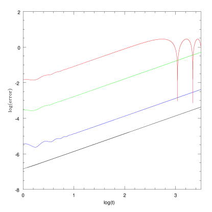
Figure 1: Here, we plot log(error) vs. log(time). Error is calculated according to Eq. (67). The lines from top to bottom correspond to the 1st, 2nd, 3rd and 4th order methods of Eqs. (60), (61), (65) and (66).

We used the first order method

$${\cal Z}_{1}^{1}=(1)=\left(e^{-i\Delta t\sigma_{x}}e^{-i\Delta t\sigma_{y}}e^{-i\Delta t\sigma_{z}}\right)$$ (60)

the second order method

$${\cal Z}_{2}^{1}=(1)(1)^{T}=\left(e^{-i\Delta t\sigma_{x}}e^{-i\Delta t\sigma_{y}}e^{-i\Delta t\sigma_{z}}\right)\left(e^{-i\Delta t\sigma_{z}}e^{-i\Delta t\sigma_{y}}e^{-i\Delta t\sigma_{x}}\right)$$ (61)

the third order method

$${\cal Z}_{3}^{1} = (1)^{T}(1)(1)(1)(1)^{T}(-2)^{T}(1)(1)(1)$$ (65)

$$= \begin{array}[]{l}\left(e^{-i\Delta t\sigma_{z}}e^{-i\Delta t\sigma_{y}}e^{-i\Delta t\sigma_{x}}\right)\left(e^{-i\Delta t\sigma_{x}}e^{-i\Delta t\sigma_{y}}e^{-i\Delta t\sigma_{z}}\right)\left(e^{-i\Delta t\sigma_{x}}e^{-i\Delta t\sigma_{y}}e^{-i\Delta t\sigma_{z}}\right)\\ \left(e^{-i\Delta t\sigma_{x}}e^{-i\Delta t\sigma_{y}}e^{-i\Delta t\sigma_{z}}\right)\left(e^{-i\Delta t\sigma_{z}}e^{-i\Delta t\sigma_{y}}e^{-i\Delta t\sigma_{x}}\right)\left(e^{2i\Delta t\sigma_{z}}e^{2i\Delta t\sigma_{y}}e^{2i\Delta t\sigma_{x}}\right)\\ \left(e^{-i\Delta t\sigma_{x}}e^{-i\Delta t\sigma_{y}}e^{-i\Delta t\sigma_{z}}\right)\left(e^{-i\Delta t\sigma_{x}}e^{-i\Delta t\sigma_{y}}e^{-i\Delta t\sigma_{z}}\right)\left(e^{-i\Delta t\sigma_{x}}e^{-i\Delta t\sigma_{y}}e^{-i\Delta t\sigma_{z}}\right)\end{array}$$

and similarly for the fourth order method

$${\cal Z}_{4}^{1}=(1)^{T}(1)(1)^{T}(-2)(1)^{T}(1)^{T}(1)^{T}(1)^{T}(1)(1)^{T}(1)(1)(1)(1)(-2)^{T}(1)(1)^{T}(1)$$ (66)

As a measure of the error, we take the difference between the $\sigma_{x}$, $\sigma_{y}$ and $\sigma_{z}$ components of the exact solution and our methods, $\Delta\sigma_{x}$, $\Delta\sigma_{y}$ and $\Delta\sigma_{z}$. We then calculate the error

$$E=\sqrt{\left(\Delta\sigma_{x}\right)^{2}+\left(\Delta\sigma_{y}\right)^{2}+\left(\Delta\sigma_{z}\right)^{2}}$$ (67)

In Fig. (1), we plot the logarithm of the error as a function of the logarithm of the time that the system was evolved for. The first order method results are uppermost and higher order results lie underneath each other with fourth order results being the lowermost plotted. $\Delta t=0.01$ for all methods.

Notice that the first order error oscillates once it reaches order $1$. The rest of the errors remain small throughout the simulation, with the fourth order error remaining below $10^{-3}$ for the entire evolution.

The error for all methods goes as $nR\left(\Delta t\right)^{o+1}$, where $n$ is the number of times the method has been applied. Therefore, $\log E=\log\left[R\left(\Delta t\right)^{o+1}\right]+\log n$. For $\Delta t=0.01$, this makes the $y$-intercept decrease by order $-2$ as the order of the method increases. Since the time evolved is proportional to $n$, the slope of the errors is $1$ for all methods.

9 Symplectic Methods

In the study of classical Hamiltonian systems, we can cast the evolution of the coordinates $q_{i}$ and momenta $p_{i}$ of fields or particles in the same language as we have done above for quantum systems.

Write $z=(q_{i},p_{i})$. Then the Hamilton equations for the system are

$$\dot{z}=\{z,H\}$$ (68)

where $\{a,b\}$ is a Poisson bracket. Now, define $D_{H}z\equiv\{z,H\}$. The Hamilton equations become

$$\dot{z}=D_{H}z$$ (69)

The formal solution to these equations is then,

$$z(t)=e^{D_{H}t}z_{0}$$ (70)

Often, $D_{H}$ can be separated into kinetic and potential parts $D_{H}=D_{K}+D_{V}$. In this case, we have the formal solution

$$z(t)=e^{(D_{K}+D_{V})t}z_{0}$$ (71)

Typically, symplectic methods approximate the above case (71), in which there are only two operators in the exponential. Symplectic methods for two operators exist up to 8th order in the expansion [11].

In our work, we have developed methods to approximate the case where there are an arbitrary number of operators in the exponential. This is important for simulations on both quantum and classical computers, since there can often be more than two terms which do not commute in the Hamiltonian.

For example, any Hamiltonian of the form

$$H=g_{ij}(q)p_{i}p_{j}+V(q)$$ (72)

where $g_{ij}$ and $V$ are functions of the $q_{i}$’s, can have an arbitrary number of terms which do not commute with each other.

A simple example of a quantum system where extra terms in the sum are necessary is an Ising spin system with next-nearest neighbor interactions. Here, the Hamiltonian becomes

$$H=\sum_{i=1}^{N}\left(\sigma_{i}\cdot\sigma_{i+1}+\sigma_{i}\cdot\sigma_{i+2}\right)$$ (73)

In this Hamiltonian, none of the terms $\sigma_{i-2}\cdot\sigma_{i}$, $\sigma_{i-1}\cdot\sigma_{i}$, $\sigma_{i}\cdot\sigma_{i+1}$ or $\sigma_{i}\cdot\sigma_{i+2}$ commute. Therefore, for this system, we can arrange the Hamiltonian to have, at best, four terms which do not commute with each other.

10 Conclusions

The object of this paper has been to provide higher order approximation methods for operators of the form $\exp{\sum_{i=1}^{N}A_{N}}$ in terms of operators of the form $\exp{(A_{1})}$, $\exp{(A_{2})}$, $\ldots$, $\exp{(A_{N})}$. We have focused on approximation methods of this kind since they are particularly useful in quantum many-particle simulations for which the discretised Hamiltonian on a quantum computer takes the form of an exponential of a sum of non-commuting terms.

To find higher order methods, we have derived and solved equations for methods up to 4th order. We find that the equations give a large number of methods, so we have selected a small number of them based on what seem to us to be reasonable criteria and presented them above.

As a by-product of our search, we have also been able to find higher order approximation methods for operators of the form $\exp{[A,B]}$ in terms of operators of the form $\exp{(A)}$ and $\exp{(B)}$. These may be useful for quantum gates where $\exp{(A)}$ and $\exp{(B)}$ are available in hardware, but the gate $\exp{[A,B]}$ is desired for some particular algorithm.

Our analysis has also shown that there is a quick technique for deriving approximation methods to arbitrarily high order involving the solution of relatively simple equations at each order. We have also presented these results, but it turns out that they lead to approximations that are far from optimal in the sense that there are many more gates in these methods than should be necessary. That is, they are accurate to high order, but relatively costly to implement.

As an example of how useful our approximations can be, let us consider a case in which we want to apply an approximation method for time $T=1$ with total error $E=10^{-4}$. For a first order method, this means that we require about $5000$ applications of the method. For second order, we require about $30$ applications. For our third order method ${\cal Z}_{3}^{1}$, we need $2$ applications. And for fourth order method ${\cal Z}_{4}^{1}$, one application of the method is more than sufficient. This results in a reduction of orders of magnitude in the computational cost of a given simulation or gate application.

Using our equations, it is possible to search for 5th order methods (and from these, via transposition, to obtain 6th order methods). We made a number of attempts at the search, but were unable to find any 5th order methods due to the large size of the search space. Thus, the only methods of 5th order and higher that we found were those methods mentioned above which tend to involve unnecessarily large numbers of gates.

Appendices

A.1   Proof of lower bounds on integral method sizes

$$\left(\sigma_{I}^{1}\right)^{p} = \sum_{i=1}^{I}\left[\left(\sigma_{i}^{1}\right)^{p}-\left(\sigma_{i-1}^{1}\right)^{p}\right]$$ (74)

$$= \sum_{i=1}^{I}\left[\left(\sigma_{i-1}^{1}+\alpha_{i}a_{i}\right)^{p}-\left(\sigma_{i-1}^{1}\right)^{p}\right]$$

$$= \sum_{i=1}^{I}\left[\sum_{q=1}^{p-1}\frac{p!}{q!(p-q)!}\left(\alpha_{i}a_{i}\right)^{q}\left(\sigma_{i-1}^{1}\right)^{p-q}+\alpha_{i}^{p}a_{i}^{p}\right]$$

$\alpha_{i}=\pm 1$. Therefore, if $p$ is odd, then

$$\sum_{i=1}^{I}\alpha_{i}^{p}a_{i}^{p}=\sum_{i=1}^{I}\alpha_{i}a_{i}^{p}=\sigma_{I}^{p}$$ (75)

and if $p$ is even, then

$$\sum_{i=1}^{I}\alpha_{i}^{p}a_{i}^{p}=\sum_{i=1}^{I}a_{i}^{p}=\sum_{i=1}^{I}\left(1-\alpha_{i}\right)a_{i}^{p}+\sum_{i=1}^{I}\alpha_{i}a_{i}^{p}=\sum_{i=1}^{I}\left(1-\alpha_{i}\right)a_{i}^{p}+\sigma_{I}^{p}$$ (76)

Taking $p=2$, the factor $\frac{p!}{q!(p-q)!}$, $q=1$, is equal to 2, and the factor $\left(1-\alpha_{i}\right)$ is 0 or 2. A 2nd-order method requires $\sigma_{I}^{2}=0$, therefore $\left(\sigma_{I}^{1}\right)^{2}$ must be even, and so $\sigma_{I}^{1}$ must also be even.

Taking $p=3$, the factors $\frac{p!}{q!(p-q)!}$, $q=1,2$, are equal to 3. A 3rd-order method requires $\sigma_{I}^{3}=0$, therefore $\left(\sigma_{I}^{1}\right)^{3}$ must be a multiple of 3, and so $\sigma_{I}^{1}$ must also be a multiple of 3.

Taking $p=4$, the factor $\frac{p!}{q!(p-q)!}$, $q=1,2,3$, is even, and the factor $\left(1-\alpha_{i}\right)$ is 0 or 2. A 4th-order method requires $\sigma_{I}^{4}=0$, therefore $\left(\sigma_{I}^{1}\right)^{4}$ must be even, and so $\sigma_{I}^{1}$ must also be even.

Taking $p=5$, the factors $\frac{p!}{q!(p-q)!}$, $q=1,2,3,4$, are multiples of 5. A 5th-order method requires $\sigma_{I}^{5}=0$, therefore $\left(\sigma_{I}^{1}\right)^{5}$ must be a multiple of 5, and so $\sigma_{I}^{1}$ must also be a multiple of 5.

Combining these $\sigma_{I}^{1}$ must be a multiple of 2 in a 2nd-order method, a multiple of 6 in a 3rd or 4th order method, and a multiple of 30 in a 5th-order method.

A.2   Formulae for the $B_{2}^{X}$’s in terms of the commutators of $A_{1}$ and $A_{2}$

The $B_{2}^{p}$ are defined by

$$e^{aA_{1}}e^{aA_{2}}=\exp\sum_{p=1}^{\infty}a^{p}B_{2}^{p}$$ (77)

The Campbell-Baker-Hausdorff formula, Eq. (4), then gives

$$B_{2}^{1} = A_{1}+A_{2}$$ (78)

$$B_{2}^{2} = \frac{1}{2}A_{12}$$ (79)

$$B_{2}^{3} = \frac{1}{12}\left(A_{112}+A_{221}\right)$$ (80)

$$B_{2}^{12}\equiv\left[B_{2}^{1},B_{2}^{2}\right] = \frac{1}{2}\left(A_{112}-A_{221}\right)$$ (81)

$$B_{2}^{4} = \frac{1}{24}A_{1221}$$ (82)

$$B_{2}^{13}\equiv\left[B_{2}^{1},B_{2}^{3}\right] = \frac{1}{12}\left(A_{1112}+A_{2221}\right)$$ (83)

$$B_{2}^{112}\equiv\left[B_{2}^{1},B_{2}^{12}\right] = \frac{1}{2}\left(A_{1112}-A_{2221}-2A_{1221}\right)$$ (84)

$$B_{2}^{5} = -\frac{1}{720}\left(A_{11112}-2A_{21112}-6A_{11221}\right.$$ (85)

$$\left.\hskip 56.9055pt\mbox{}-6A_{22112}-2A_{12221}+A_{22221}\right)$$

$$B_{2}^{14}\equiv\left[B_{2}^{1},B_{2}^{4}\right] = \frac{1}{24}\left(A_{11221}-A_{22112}\right)$$ (86)

$$B_{2}^{23}\equiv\left[B_{2}^{2},B_{2}^{3}\right] = \frac{1}{24}\left(\left[A_{12},A_{112}\right]+\left[A_{12},A_{221}\right]\right)$$ (87)

$$= -\frac{1}{24}\left(A_{21112}+A_{11221}-A_{22112}-A_{12221}\right)$$

$$B_{2}^{113}\equiv\left[B_{2}^{1},B_{2}^{13}\right] = \frac{1}{12}\left(A_{11112}+A_{21112}+A_{12221}+A_{22221}\right)$$ (88)

$$B_{2}^{221}\equiv-\left[B_{2}^{2},B_{2}^{12}\right] = \frac{1}{4}\left(-\left[A_{12},A_{112}\right]+\left[A_{12},A_{221}\right]\right)$$ (89)

$$= \frac{1}{4}\left(A_{21112}+A_{11221}+A_{22112}+A_{12221}\right)$$

$$B_{2}^{1112}\equiv\left[B_{2}^{1},B_{2}^{112}\right] = \frac{1}{2}\left(A_{11112}+A_{21112}-2A_{11221}\right.$$ (90)

$$\left.\hskip 56.9055pt\mbox{}+2A_{22112}-A_{12221}-A_{22221}\right)$$

A.3   A simple measure of the error

The error for a given method is given by Eq. (15)

$$r=\sum_{X}\sigma_{I}^{X}B_{N}^{X}$$ (91)

where $X\in\{4,13,112\}$ for a 3rd order method and $X\in\{5,14,23,113,221,1112\}$ for a 4th order method.

$r$ is a vector in the vector space of the commutators for which we do not know the metric. We would like to have a scalar measure of the error, and thus must pick some basis for the vector space. We choose the basis to be the commutators of $A_{1}$ and $A_{2}$. This basis is simple and spans the vector space of the $B_{N}^{X}$’s without redundancy. Since this basis spans the space of the $B_{N}^{X}$’s, we do not need to go to $N$ larger than $2$. For $N=2$, we can re-express $r$ as

$$r=\sum_{Y}\rho_{Y}A_{Y}$$ (92)

where

$$Y\in\{1112,1221,2221\}$$ (93)

for a 3rd order method and

$$Y\in\{11112,21112,11221,22112,12221,22221\}$$ (94)

for a 4th order method. The formulae for the $\rho_{Y}$’s in terms of the $\sigma_{I}^{X}$’s are given in Appendix A.4. In this basis, our measure of the error then becomes

$$R\equiv\sqrt{\sum_{Y}(\rho_{Y})^{2}}$$ (95)

A.4   Formulae for the $\rho_{Y}$’s in terms of the $\sigma_{I}^{X}$’s

For $N=2$,

$$r=\sum_{X}\sigma_{I}^{X}B_{2}^{X}=\sum_{Y}\rho_{Y}A_{Y}$$ (96)

Therefore, using the formulae in Appendix A.2, we obtain

$$\rho_{1} = \sigma_{I}^{1}$$ (97)

$$\rho_{2} = \sigma_{I}^{1}$$ (98)

$$\rho_{12} = \frac{1}{2}\sigma_{I}^{2}$$ (99)

$$\rho_{112} = \frac{1}{12}\sigma_{I}^{3}+\frac{1}{2}\sigma_{I}^{12}$$ (100)

$$\rho_{221} = \frac{1}{12}\sigma_{I}^{3}-\frac{1}{2}\sigma_{I}^{12}$$ (101)

$$\rho_{1112} = \frac{1}{12}\sigma_{I}^{13}+\frac{1}{2}\sigma_{I}^{112}$$ (102)

$$\rho_{1221} = \frac{1}{24}\sigma_{I}^{4}-\sigma_{I}^{112}$$ (103)

$$\rho_{2221} = \frac{1}{12}\sigma_{I}^{13}-\frac{1}{2}\sigma_{I}^{112}$$ (104)

$$\rho_{11112} = -\frac{1}{720}\sigma_{I}^{5}+\frac{1}{12}\sigma_{I}^{113}+\frac{1}{2}\sigma_{I}^{1112}$$ (105)

$$\rho_{21112} = \frac{1}{360}\sigma_{I}^{5}-\frac{1}{24}\sigma_{I}^{23}+\frac{1}{12}\sigma_{I}^{113}+\frac{1}{4}\sigma_{I}^{221}+\frac{1}{2}\sigma_{I}^{1112}$$ (106)

$$\rho_{11221} = \frac{1}{120}\sigma_{I}^{5}+\frac{1}{24}\sigma_{I}^{14}-\frac{1}{24}\sigma_{I}^{23}+\frac{1}{4}\sigma_{I}^{221}-\sigma_{I}^{1112}$$ (107)

$$\rho_{22112} = \frac{1}{120}\sigma_{I}^{5}-\frac{1}{24}\sigma_{I}^{14}+\frac{1}{24}\sigma_{I}^{23}+\frac{1}{4}\sigma_{I}^{221}+\sigma_{I}^{1112}$$ (108)

$$\rho_{12221} = \frac{1}{360}\sigma_{I}^{5}+\frac{1}{24}\sigma_{I}^{23}+\frac{1}{12}\sigma_{I}^{113}+\frac{1}{4}\sigma_{I}^{221}-\frac{1}{2}\sigma_{I}^{1112}$$ (109)

$$\rho_{22221} = -\frac{1}{720}\sigma_{I}^{5}+\frac{1}{12}\sigma_{I}^{113}-\frac{1}{2}\sigma_{I}^{1112}$$ (110)

A.5   Tables of Residual Errors

3rd Order Integer Methods

	$\rho_{1}$	$\rho_{1112}$	$\rho_{1221}$	$\rho_{2221}$
${\cal Z}_{3}^{1}$	6.0	-1.0	0.5	0.0
${\cal Z}_{3}^{2}$	12.0	-4.0	-3.0	5.0
${\cal Z}_{3}^{3}$	6.0	-2.0	1.5	1.0
${\cal Z}_{3}^{4}$	6.0	0.0	4.5	9.0
${\cal Z}_{3}^{5}$	12.0	-864.0	792.0	180.0

	$\rho_{11112}$	$\rho_{21112}$	$\rho_{11221}$	$\rho_{22112}$	$\rho_{12221}$	$\rho_{22221}$
${\cal Z}_{3}^{1}$	2.2	3.1	-3.2	5.3	0.1	-1.3
${\cal Z}_{3}^{2}$	13.4	104.2	105.6	26.1	84.2	28.9
${\cal Z}_{3}^{3}$	0.7	5.1	3.3	1.8	3.1	1.2
${\cal Z}_{3}^{4}$	2.7	8.1	-2.7	10.8	-6.9	-13.8
${\cal Z}_{3}^{5}$	-3801.6	-1900.8	2505.6	-1166.4	499.2	206.4

3rd Order Irrational Method

	$\rho_{1}$	$\rho_{1112}$	$\rho_{1221}$	$\rho_{2221}$
${\cal R}_{3}^{1}$	1.0	0.012008	-0.052816	-0.058414

	$\rho_{11112}$	$\rho_{21112}$	$\rho_{11221}$	$\rho_{22112}$	$\rho_{12221}$	$\rho_{22221}$
${\cal R}_{3}^{1}$	0.001754	0.003500	-0.009304	0.017412	-0.014311	-0.026310

4th Order Integer Methods

	$\rho_{1}$	$\rho_{11112}$	$\rho_{21112}$	$\rho_{11221}$	$\rho_{22112}$	$\rho_{12221}$	$\rho_{22221}$
${\cal R}_{4}^{1}$	12.0	-1.6	0.2	-3.4	5.6	-1.8	-2.6
${\cal R}_{4}^{2}$	12.0	3.4	6.2	3.6	3.6	2.2	-4.6
${\cal R}_{4}^{3}$	12.0	26.4	40.2	-5.4	21.6	16.2	5.4
${\cal R}_{4}^{4}$	12.0	-369.6	-220.8	309.6	-86.4	259.2	86.4

4th Order Irrational Methods

	$\rho_{1}$	$\rho_{11112}$	$\rho_{21112}$	$\rho_{11221}$	$\rho_{22112}$	$\rho_{12221}$	$\rho_{22221}$
${\cal R}_{4}^{1}$	1.0	-0.000414	-0.008682	-0.007027	-0.026045	-0.026732	-0.004684
${\cal R}_{4}^{2}$	1.0	-0.022171	-0.013256	0.014902	-0.009176	0.002796	0.001717
${\cal R}_{4}^{3}$	1.0	-0.001297	0.038072	0.035227	-0.080082	-0.079215	0.001270
${\cal R}_{4}^{4}$	1.0	0.002074	0.196582	0.194095	-0.052861	-0.050727	-0.002155

References

- [1] P. W. Shor, in Proceedings of the 35th Annual Symposium on Foundations of Computer Science, Santa Fe, NM, 1994, edited by Shafi Goldwasser (IEEE Computer Society Press, Los Alamitos, CA, 1994), 124-134; SIAM J. Comput. 26, 1484-1509 (1997).
- [2] J. Preskill, quant-ph/9712048.
- [3] R. Laflamme, E. Knill, W. H. Zurek, T. F. Havel and S. S. Somaroo, Phys. Rev. Lett. 81, 2152-2155 (1998).
- [4] L. Grover, Phys. Rev. Lett. 79, 325-328 (1997).
- [5] B. M. Boghosian and W. Taylor IV, quant-ph/9701019; quant-ph/9701016; quant-ph/9604035; D. S. Abrams and S. Lloyd, Phys. Rev. Lett. 79, 2589-2589 (1997).
- [6] R. P. Feynman, Int. Jour. of Theor. Phys. 21, 467-488 (1982).
- [7] D. S. Abrams and S. Lloyd, Phys. Rev. Lett. 79, 2586-2589 (1997).
- [8] A. Steane, quant-ph/9708022; S. Lloyd, Phys. Rev. Lett. 75, 346-349 (1995); D. Deutsch, A. Barenco and A. Ekert, quant-ph/9505018; A. Barenco, et. al., quant-ph/9503016.
- [9] D. Goldman and T. Kaper, SIAM J. Num. Anal. 33, 349-367 (1996). M. Suzuki, Phys. Lett. A 146, 319-323 (1990); M. Suzuki, J. Math. Phys. 32, 400-407 (1991);
- [10] Numerical Recipes, The Art of Scientific Computing, W. H. Press, S. A. Teukolsky, W. T. Vetterling and B. P. Flannery, Cambridge University Press, 376-381 (1992).
- [11] H. Yoshida, Phys. Lett. A 150, 262-268 (1990).