Quantum interference by two temporally distinguishable pulses

Abstract

We report a two-photon interference effect, in which the entangled photon pairs are generated from two laser pulses well-separated in time. In a single pump pulse case, interference effects did not occur in our experimental scheme. However, by introducing a second pump pulse delayed in time $T$, quantum interference was then observed. The visibility of the interference fringes shows dependence on the delay time $T$ between two laser pulses. The results are explained in terms of indistinguishability of biphoton amplitudes which originated from two temporally separated laser pulses.

The superposition principle plays the central role in interference phenomena in quantum mechanics. In a quantum mechanical picture, interference occurs because there are indistinguishable ways of an event to occur [1]. Classically, one would not expect to observe interference from two temporally separated laser pulses. To observe interference the two pulses, if coherent, must be brought back together in space or “spread” by a narrow-band filter. However, it is possible to observe interference effects for entangled two-photon states generated by two laser pulses which are well-separated in time.

In this paper, we report a quantum interference experiment in which the interference occurs between amplitudes of entangled two-photon states generated by two temporally well-separated laser pulses. The delay between the two pump laser pulses is chosen to be much greater than the width of the pump pulse and the width of the “wavepacket” determined by the spectral filter used in front of the detectors. Therefore, the “wavepackets” are well distinguishable from single-photon point of view. We first show why interference effects are not expected for the case of a single pump pulse in our experimental setup. Then we introduce a second pump pulse delayed in time $T$ and show how one can recover quantum interference. In this sense, this experiment can be viewed as a temporal quantum eraser.

The two-photon state in this experiment is generated by spontaneous parametric down conversion (SPDC). SPDC is a nonlinear optical process in which a higher energy UV pump photon is converted to a pair of lower energy photons (usually called signal, and idler) inside a non-centrosymmetric crystal (in this case, $\beta-BaB_{2}O_{4}$, called “BBO”), when the phase matching condition ($\omega_{p}=\omega_{s}+\omega_{i}$, $\vec{k}_{p}=\vec{k}_{s}+\vec{k}_{i}$, where the subscripts refer to the pump, signal, and idler) is satisfied [2]. Signal

and idler have the same polarization in type I SPDC, and orthogonal polarization in type II SPDC.

Let us first consider the case in which a single pump pulse is used for a SPDC process in the experimental setup shown in Fig. 1. A pair of SPDC photon is fed into the interferometer. Two photon counting detectors are placed at the two output ports of the interferometer. The coincidences between the two detectors are recorded. There are two biphoton amplitudes which could result in coincidence counts for this interferometer: both signal and idler are (1) transmitted (t-t), (2) reflected (r-r) at the beamsplitter (BS). If the pump is CW, interference between amplitudes t-t and r-r may occur. Due to the long coherence length of the pump, the two biphoton amplitudes t-t and r-r may be indistinguishable, although delays $\tau$ and $\tau_{1}$ are introduced as shown in Fig. 1 [3]. However, when a short pulse pump is used, the interference can never occur. It is, in principle, possible to know which path (t-t or r-r) the pair took to contribute a coincidence count. See the Feynman diagrams in Fig. 2. One can distinguish t-t and r-r amplitudes by measuring the time difference between the pulse pump and the detection at one detector since the pump pulse acts as a clock fixing the origin of the biphoton. In other words, the Feynman alternatives which originated from a single pulse are distinguishable. It is clear that no interference will be observed in this case.

In a formal quantum mechanical representation [4], the field at the detectors can be written as:

$$E_{1}^{(+)}(t_{1}) = \frac{1}{\sqrt{2}}\sum_{\omega}e_{\omega}\left((\hat{e}_{x}\cdot\hat{e}_{1})a_{1s}(k(\omega))e^{-i\omega(t_{1}-\tau_{1})}\right.$$ (1)

$$+ \left.i(\hat{e}_{y}\cdot\hat{e}_{1})a_{1i}(k(\omega))e^{-i\omega(t_{1}-\tau)}\right)\quad,$$ (2)

$$E_{2}^{(+)}(t_{2}) = \frac{1}{\sqrt{2}}\sum_{\omega}e_{\omega}\left((\hat{e}_{y}\cdot\hat{e}_{2})a_{2i}(k(\omega))e^{-i\omega(t_{2}-\tau)}\right.$$ (3)

$$+ \left.i(\hat{e}_{x}\cdot\hat{e}_{2})a_{2s}(k(\omega))e^{(-i\omega t_{2})}\right)\quad,$$ (4)

where, for example, $a_{1s}(k(\omega))$ is the annihilation operator of a photon arriving at $D_{1}$ from the transmitted beam $s$ with wave number $k(\omega)$, $e_{\omega}=\sqrt{\frac{\hbar\omega}{2\epsilon_{0}V_{Q}}}$, $V_{Q}$ is the quantization volume, and $t_{i}=T_{i}-\frac{l_{i}}{c}$, $i=1,2$ with $l_{i}$ denoting the optical path length from the output face of the crystal to detector $i$. $\hat{e}_{x}$ and $\hat{e}_{y}$ are the unit vectors representing the polarization of the photons and $\hat{e}_{1}$ and $\hat{e}_{2}$ are the unit vectors representing the orientations of the analyzers placed in front of the detectors. We can define the scalar projections of the polarizations onto the detector analyzers as $\hat{e}_{x}\cdot\hat{e}_{i}=\cos\theta_{i}$ and $\hat{e}_{y}\cdot\hat{e}_{i}=\sin\theta_{i}$, where $i=1,2$. The coincidence counting rate is given by integrals over the firing times of the two detectors, $T_{1},T_{2}$ respectively [5]:

$$R_{c} \propto \frac{1}{T}\int_{0}^{T}dT_{1}dT_{2}\langle\Psi|E_{1}^{(-)}E_{2}^{(-)}E_{2}^{(+)}E_{1}^{(+)}|\Psi\rangle$$ (5)

$$= \frac{1}{T}\int_{0}^{T}dT_{1}dT_{2}\left|\langle 0|E_{2}^{(+)}E_{1}^{(+)}|\Psi\rangle\right|^{2}\quad.$$ (6)

In our experiment, the pump pulse is linearly polarized and propagating in the $z$-direction. The central frequency of the pump pulse is $\Omega_{p}$ and it has an envelope of arbitrary shape, $\tilde{E}_{p}$. Then the pump pulse field can be defined by

$$E_{p}(z,t) = e^{-i\Omega_{p}t}\tilde{E}_{p}(z,t)\quad,$$ (7)

$$\tilde{E}_{p}(z,t) = \int d\nu_{p}\bar{E}_{p}(\nu_{p})e^{ik_{p}(\Omega_{p}+\nu_{p})z-i\nu_{p}t}\quad.$$ (8)

The SPDC state vector is given by

$$|\Psi\rangle=|0\rangle+g\sum_{k_{s},k_{i}}\bar{E}_{p}(\omega_{i}+\omega_{s}-\Omega_{p})\times$$ (9)

$$a_{s}^{\dagger}(k_{s}(\omega_{s}))a_{i}^{\dagger}(k_{i}(\omega_{i}))|0\rangle\quad,$$ (10)

where $|0\rangle$ is the vacuum state, and all constants have been gathered in $g$. Here we consider the degenerate case ($\omega_{i}=\omega_{s}$). Let us define $t_{+}\equiv\frac{1}{2}(t_{1}+t_{2}-2\tau),t_{12}\equiv t_{1}-t_{2}+\tau.$ If $t_{12}$ is positive, the idler arrives after the signal. We may think of $t_{+}$ as the mean time at which the two-photon wavepacket arrives at the detectors. The biphoton wavepackets are “superposed” in the form:

$$\langle 0|E_{2}^{(+)}E_{1}^{(+)}|\Psi\rangle= - \sin\theta_{1}\cos\theta_{2}A(t_{+}-\tau_{1},t_{12}-2\tau+\tau_{1})$$ (11)

$$+ \cos\theta_{1}\sin\theta_{2}A(t_{+},-t_{12})\quad.$$ (12)

In Eq. (12) the first term represents the amplitude (wavepacket) where both signal and idler are transmitted (t-t) at the beamsplitter (BS) and the second term represents the amplitude (wavepacket) where both signal and idler are reflected (r-r) at the beamsplitter. Here we have considered only the terms which could result in coincidence counts. To observe interference, the t-t and the r-r biphoton amplitudes must be indistinguishable for a given detection time pair ($t_{1},t_{2}$). Indistinguishability of the two Feynman alternatives implies that it is impossible to tell the biphoton path from the detection times. It can be shown [4] that the two biphoton amplitudes cannot be indistinguishable when we choose a delay $\tau>\sigma_{pulse}$, the pump pulse width, as in our experiment. Thus the interference cannot occur in our experimental setup from a single pulse pump.

Now, we might ask ourselves, in the case of $\tau>\sigma_{pulse}$, whether it is possible to “recover” the quantum interference. This can be accomplished by introducing a second pulse delayed in time $T$ with $T=\tau>\sigma_{pulse}$. This solution may come with a serious question: Can interference occur between two temporally distinguishable pulses? The answer is yes. Fig. 3 shows the Feynman diagrams for this two-pulse-pump scheme. The complete theoretical treatment can be found in [4]. The condition for interference is found to be:

$$T=\tau,\quad 2\tau=\tau_{1}\quad.$$ (13)

When this condition is satisfied, even though (1) the two pump pulses are well distinguishable in time, (2) detection events for signal or idler are distinguishable, the r-r amplitude from the first pulse and the t-t amplitude from the second pulse are indistinguishable with respect to the coincidence detections. This is illustrated in Fig. 3. This is a two-photon interference phenomenon between biphoton amplitudes which originated from two temporally well-separated pulses.

It can be easily shown that the maximum visibility of the interference fringe for two pulses is $50\%$ by simply using the Feynman diagrams shown in Fig. 3. The coincidence counting rate is proportional to $\left|\langle 0|E_{2}^{(+)}E_{1}^{(+)}|\Psi\rangle\right|^{2}$,

$$R_{c}\propto|A_{1tt}+A_{2tt}+A_{1rr}+A_{2rr}|^{2}\quad,$$ (14)

where $A_{1}$ and $A_{2}$ represent the biphoton amplitudes resulting from the first and the second pulse pump, respectively. Subscripts $tt$ and $rr$ simply refer to transmitted-transmitted and reflected-reflected. Considering the non-zero terms of Eq. (14) only,

$$R_{c}\propto 4+A_{2tt}A_{1rr}^{*}+A_{1rr}A_{2tt}^{*}\quad,$$ (15)

which shows $50\%$ visibility at maximum if $A_{2tt}$ and $A_{1rr}$ overlap. This deserves further comments. It is usually understood that quantum phenomena show $100\%$ maximum visibility while classical correlation of fields shows $50\%$ maximum visibility in fourth-order interference experiments [6]. In our case, however, maximum visibility is $50\%$ although the interference is purely quantum mechanical in nature: it is due to the quantum entanglement. If we consider multiple pulses ($N>2$) delayed in time $T$ with respect to one another and include more biphoton amplitudes, maximum visibility can reach $100\%$ [4]. When $N$ pulse pumps are considered, the visibility is given by:

$$V(\Delta m,N)=\frac{N-\Delta m}{N}\quad,$$ (16)

where $\Delta m$ is the difference in pulse numbers of the involved pump pulses. (For adjacent pulses, $\Delta m=1$.)

In our experiment, two temporally separated pump pulses were obtained by transmitting a single pump pulse through a quartz rod with the optic axis normal to the pump beam and rotated by 45 deg with respect to the pump polarization. See Fig. 4a. Since the e-ray and o-ray inside the quartz propagate with different group velocities, the incident single pulse starts to separate into two pulses. The length of the quartz rod controls the delay between the two output pulses: one polarized in the fast axis direction and the other polarized in the slow axis direction of the quartz rod. We can further vary this delay by placing quartz plates after the quartz rod to either make the delay bigger (optic axis parallel to that of the quartz rod) or smaller (optic axis perpendicular to that of the quartz rod). The repetition rate of the original pump pulse is about $90MHz$, so the distance between adjacent pulse is about $11nsec.$ The single pump pulse has about $140fsec.$ width and central wavelength of $400nm$. The delay ($T$) between the two pulses is varied from $160\mu m\sim 280\mu m$ (or $533fsec.\sim 933fsec.$), and a coincidence time window of $3ns$ is used. Therefore we can safely say that the two pulses are temporally well-separated and we only accept biphoton amplitudes originating from two neighboring pump pulses.

In the experiment, we made use of type II degenerate collinear SPDC ($\lambda_{s}=\lambda_{i}=2\lambda_{p}$, where $s$, $i$, and $p$ stands for signal, idler, and pump respectively). The schematic of the experiment is shown in Fig. 4b. In this scheme, an orthogonal polarized signal-idler photon pair (one with horizontal polarization, and the other with vertical polarization with respect to the optic table) propagates in the same direction as the pump. The thickness of the BBO crystal used in the experiment was $100\mu m$ and the filter bandwidth was chosen to be $10nm$ ($l_{coh}\simeq\lambda^{2}/\Delta\lambda\simeq 64\mu m$). The interferometer consists of many quartz rods and quartz plates. If the quartz rods (plates) are placed with optic axis parallel or perpendicular to that of the BBO crystal, they introduce delays between the signal-idler photon pair. The first delay ($\tau$: QR1 and QP1) is chosen to be $197\mu m$ (or $657fsec.$) and the second delay ($\tau_{1}$: QR2, QR3, QP2, and QP3) is chosen to be $2\times 197\mu m$. So, here we satisfy one of the two conditions to observe two-photon interference from two separate pulses, which is $\tau_{1}=2\tau$. $\tau$ delays idler relative to signal and $\tau_{1}$ delays signal relative to idler.

To demonstrate the two-photon interference effects, we first show the polarization interference. The analyzer $A_{2}$ is fixed at $45^{o}$ and $A_{1}$ is rotated while recording the coincidence and single counts. The single counting rate of the detector $D_{1}$ is found to be almost constant while the coincidence counts show $\sin^{2}(\theta_{1}-\theta_{2})$ or $\sin^{2}(\theta_{1}+\theta_{2})$ modulation depending on the phases introduced when changing the inter-pulse delay $T$ [3, 7, 8]. We record the visibility of this polarization interference while varying the delay $T$ between the two pulses. This is shown in Fig. 5. It is clearly shown that when the delay $T$ is equal to the interferometer delay $\tau$, the maximum visibility, which in this case is $33\%$, is observed.

We also observed the dependence of coincidence counting rate on the phase shift between the two pump pulses: the space-time interference [8]. This is done by orienting the two polarizers ($A_{1}$ and $A_{2}$) at $45^{o}$ and by placing two additional quartz plates after QR1. By tilting the quartz plates, we introduce additional phase delay between the pump pulses. From eqs. (12) and (15), we expect to observe,

$$R_{c}\propto 4-2\eta(T)\cos(\Omega_{p}\phi_{p})\quad,$$ (17)

where $\Omega_{p}$ is the pump frequency, $\phi_{p}$ is the pump phase, and $\eta(T)$ has a value of $0\sim 1$ and reflects the fact that the visibility of the interference fringe depends on the value of the inter-pulse delay $T$. For the case of maximum visibility, $\eta(\tau)=1$. The data shown in Fig. 6 demonstrates dependence on pump phase change. The modulation period is $400nm$ (pump wavelength) as expected from Eq. (17). Data shown in Figs. 5 and 6 clearly demonstrate two-photon interference effects between biphoton amplitudes generated from two temporally separated pump pulses.

In conclusion, we have experimentally demonstrated the two-photon interference between biphoton amplitudes arising from two temporally well-separated pump pulses. It is important to note the following. (1) The pump pulse intensity was low enough so that single counting rates of the detectors were kept much smaller than the pulse repetition rate: the probability of having one SPDC photon pair per pulse in our experiment is negligible. Hence the interference cannot be explained as two SPDC photons from two pump pulses (one SPDC pair from each pulse) interfering at the detectors. The two pump pulses simply provide two biphoton amplitudes which could result in coincidence counts, and interference occurs between these two biphoton amplitudes only when they are indistinguishable. (2) The BBO crystal in our experiment was only $100\mu m$ thick, so the two-pulse did not exist in the BBO at the same time at any moment. (3) Due to the delays in the interferometer ($\tau$, $\tau_{1}$), the signal and idler never met at the beamsplitter (BS). Therefore, the existence of two-photon interference cannot be viewed as the interference between the signal and idler photons. These three points again emphasize the fact that it is the indistinguishability of the Feynman alternatives for the biphoton amplitudes which is responsible for the quantum interference effects.

This work was supported, in part, by the U.S. Office of Naval Research, and the National Security Agency. MVC and SPK would like to thank the Russian Foundation for Basic Research, Grant # 97-02-17498 for supporting their visit to Univ. of Maryland, Baltimore County.

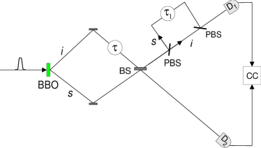
FIG. 1.: Schematic of the experiment.

FIG. 2.: Feynman diagrams for the single pulse case. Two amplitudes are distinguishable since the pump pulse acts as a clock.

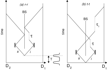
FIG. 3.: Feynman diagrams for the two-pulse case. r-r (1st pulse) and t-t (2nd pulse) are indistinguishable in terms of the detector firing times.

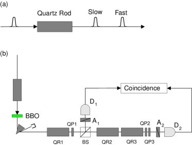
FIG. 4.: (a) Scheme to produce a train of two pulses. See text for details. (b) Experimental setup. Each detector package consists of a short focus lens, an interference filter with $10nm$ FWHM, and an avalanche photo-diode.

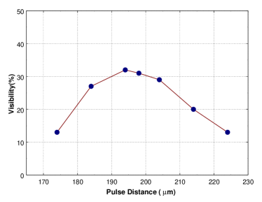
FIG. 5.: Visibility change of the polarization interference while the delay between two pulses is varied. When $T=\tau$, maximum visibility was observed.

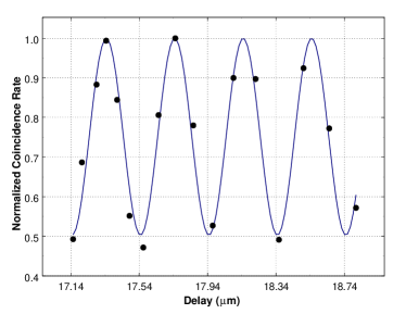
FIG. 6.: Space-time interference showing dependence on pump phase. The modulation period is $400nm$ as expected from Eq. (17).

REFERENCES

- [1] R.P. Feynman, QED The Strange Theory of Light and Matter (Princeton Univ. Press, Princeton, NJ, 1985)
- [2] D.N. Klyshko, Photon and Nonlinear Optics (Gordon and Breach Science, New York, 1988).
- [3] T.B. Pittman, et al., Phys. Rev. Lett. 77, 1917 (1996).
- [4] T.E. Keller, et al., Phys. Lett. A, 244, 507 (1998).
- [5] R.J. Glauber, Phys. Rev. 130, 2529 (1963); 131 , 2766 (1963).
- [6] L. Mandel, Phys. Rev. A 28, 929 (1983); R. Ghosh and L. Mandel, Phys. Rev. Lett. 59, 1903 (1987).
- [7] Y.H. Shih and A. V. Sergienko, Phys. Lett. A 186, 29 (1994), Y.H. Shih, et al., Phys. Rev. A 50, 23 (1994), P.G. Kwiat, et al., Phys. Rev. Lett. 75, 4337 (1995).
- [8] Y.H. Shih, et al., Phys. Rev. A 47, 1288 (1993); T.B. Pittman, et al., Phys. Rev. A 51, 3495 (1995); D.V. Strekalov, et al., Phys. Rev. A 54, R1 (1996).