Creation of coherence in Bose-Einstein condensates by atom detection

Abstract

We investigate the creation of a relative phase between two Bose-Einstein condensates, initially in number states, by detection of atoms and show how the system approaches a coherent state. Two very distinct time scales are found: one for the creation of the interference is of the order of the detection time for a few single atoms and another, for the preparation of coherent states, of the order of the detection time for a significant fraction of the total number of atoms. Approximate analytic solutions are derived and compared with exact numerical results.

PACS number(s): 03.75.Fi, 05.30.Jp, 42.50.Ar

I Introduction

The first experimental realisations of Bose-Einstein condensation in dilute atomic gases [1, 2, 3] have opened up a new field in atomic and quantum physics. Despite its apparent complexity, the condensate is well-described by a macroscopic wavefunction, or complex field, obeying a nonlinear wave equation (the Gross-Pitaevskii equation). The nature of this complex field and in particular its apparent phase has been the subject of some debate.

One specific topic which has been frequently investigated is the question of the coherence properties [4, 5] of Bose-Einstein condensates as established in interference experiments [6, 7]. The underlying question is whether the phase or, more precisely, the relative phase of two condensates is created by a spontaneously broken symmetry [8] or by some other mechanisms [9]. It has been suggested [10] (and studied in detail by several authors [11, 12, 13, 14, 15, 16]) that such a relative phase can be created by the detections of individual atoms in an interferometric setup, that is, where the origin of the detected atoms is intrinsically unknown. This process gives rise to a definite (but unpredictible) relative phase of two condensates even if the initial states of the condensates are of undefined phase, as for initial number states [10, 11, 13], initial Poissonian states [12, 14], or initial thermal states [14], by entangling the states of the two condensates.

In this work we will study in detail the creation of coherence between two condensates which initially have well defined occupation numbers, not only in the limit where the number of atoms detected is small compared to the total number of atoms but also in the long time limit. We concentrate thereby on two manifestations of coherence: the creation of interference fringes and the evolution of the compound two-condensate system towards a kind of coherent state. We start with an idealized model (Secs. III-IV) and later introduce more realistic features including atomic collisions (Sec. V). We use exact numerical simulations combined with approximate analytical solutions to determine the time evolution of our system. We show that these two measures of coherence are created on very different time scales. The relative phase associated with the appearance of interference fringes develops in a time of order $1/(N\gamma)$, where $N$ is the total initial number of atoms in the two condensates and $\gamma$ is the rate at which atoms leak out of the condensates and are detected. The approach towards coherent states, in contrast, takes a larger time of order $1/\gamma$. These two timescales correspond to timescales recently identified for the interaction of a Bose-Einstein condensate or other bosonic system with its environment [17]. In this case, a well-specified atom number will change on the timescale $1/(N\gamma)$ but any coherence present decays on a timescale $1/\gamma$.

II Model

Let us first introduce the model system which we use to investigate the coherence properties in Bose-Einstein condensation [10, 11, 12, 13, 14, 15, 16]. We consider two independent non-interacting single-mode Bose-Einstein condensates with creation (annihilation) operators $a^{\dagger}$ ($a$) and $b^{\dagger}$ ($b$), respectively. Atoms are leaking out of the condensates and are detected individually and spatially resolved. The same detectors simultaneously monitor decays from both condensates, that is, atoms coming from different condensates are allowed to interfere, see Fig. 1. Thus, the detections are described by the annihilation operators

$$a(\phi)=\frac{1}{\sqrt{2}}\left(a+be^{-i\phi}\right)$$ (1)

where $\phi\in[-\pi,\pi]$ is related to the position of the detector $x$ by $\phi=px/\hbar$ where $p$ is the momentum of the atoms leaking out of the condensates.

Assume now that the system can be described at a certain time $t$ by a wave function $|\psi\rangle$. Then the probability of detecting the next atom at position $\phi$ is given by

$$P(\phi)={\cal N}\langle\psi|a(\phi)^{\dagger}a(\phi)|\psi\rangle$$ (2)

where the normalisation constant ${\cal N}$ is chosen such that

$$\int_{-\pi}^{\pi}d\phi\,P(\phi)=1.$$ (3)

This probability function can be rewritten as

$$P(\phi)=\frac{1}{2\pi}\left[1+\beta_{c}\cos(\phi-\theta)\right]$$ (4)

where

$$\beta_{c}=\frac{2|\langle\psi|a^{\dagger}b|\psi\rangle|}{\langle\psi|a^{\dagger}a+b^{\dagger}b|\psi\rangle}$$ (5)

is the visibility of the interference fringes conditioned on the quantum state $|\psi\rangle$, and $\theta$ gives the most likely position of detection of the next atom. It should be emphasized that this visibility is not the one obtained by detecting a large number of atoms from the initial state $|\psi\rangle$, but the one obtained by preparing this state $|\psi\rangle$ very often and measuring a single atom in each run. This difference is important since every detection changes the state of the system and thus changes the conditional visibility $\beta_{c}$.

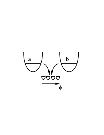
FIG. 1.: Schematic representation of the interfering Bose-Einstein condensates.

This system has already been investigated by several authors [10, 11, 12, 13, 14, 15, 16] in order to show that the detection of atoms breaks the underlying symmetry of the system and thus creates interference fringes. This is true even if the initial state of the system does not exhibit any prefered phase so that $\beta_{c}=0$. It is the main purpose of our work to quantify this creation of coherence between two initially uncorrelated Bose-Einstein condensates.

III Creating interference from initial number states

In this section we will discuss the creation of interference fringes as a consequence of consecutive detections of atoms when the two condensates are initially in number states. The full system is given initially by the quantum state

$$|\psi_{0}\rangle=|n_{1},n_{2}\rangle.$$ (6)

After the detection of $k$ atoms at positions $\phi_{1}$, $\phi_{2}$, …, $\phi_{k}$ the (unnormalized) state of the system is then

$$|\psi_{k}\rangle=(a+be^{i\phi_{k}})\dots(a+be^{i\phi_{1}})|\psi_{0}\rangle.$$ (7)

The conditional probability of detecting the $(k+1)$th atom at $\phi_{k+1}$ then reads

$$P(\phi_{k+1}|\phi_{k},...,\phi_{1})=$$ (8)

$$\quad\quad=\frac{1}{2\pi}\frac{\langle\psi_{k}|(a^{\dagger}+b^{\dagger}e^{-i\phi_{k+1}})(a+be^{i\phi_{k+1}})|\psi_{k}\rangle}{\langle\psi_{k}|a^{\dagger}a+b^{\dagger}b|\psi_{k}\rangle}$$ (9)

$$\quad\quad=\frac{1}{2\pi}\frac{\langle\psi_{k+1}|\psi_{k+1}\rangle}{(N-k)\langle\psi_{k}|\psi_{k}\rangle}$$ (10)

where $N=n_{1}+n_{2}$. Thus, the probability for the sequence of detections $\phi_{1}$, $\phi_{2}$, …, $\phi_{k}$ is

$$P(\phi_{k},...,\phi_{1})=P(\phi_{1})P(\phi_{2}|\phi_{1})...=$$ (11)

$$\quad\quad=\frac{1}{(2\pi)^{k}}\frac{\langle\psi_{k}|\psi_{k}\rangle}{N(N-1)...(N-k+1)}.$$ (12)

The conditional visibility $\beta$ (we will write $\beta$ instead of $\beta_{c}$ in this section in order to simplify the notation) for the state after $k$ detections is

$$\beta=\frac{2|\langle\psi_{k}|a^{\dagger}b|\psi_{k}\rangle|}{\langle\psi_{k}|a^{\dagger}a+b^{\dagger}b|\psi_{k}\rangle}=\frac{2|\langle\psi_{k}|a^{\dagger}b|\psi_{k}\rangle|}{(N-k)\langle\psi_{k}|\psi_{k}\rangle}.$$ (13)

Thus the average visibility after $k$ detections is

$$\langle\beta\rangle_{k}=\int d\phi_{1}...d\phi_{k}\frac{2}{(2\pi)^{k}}\frac{(N-k-1)!}{N!}|\langle\psi_{k}|a^{\dagger}b|\psi_{k}\rangle|.$$ (14)

Note, however, that this mean conditional visibility is rather difficult to access experimentally since it involves the averaging over ensembles of experiments where each ensemble consists of repeatedly preparing the quantum state of the system by the same sequence of detections from the same initial number state and measuring the position of the next detection. Nevertheless, this proves to be a useful measure theoretically especially to describe the time scale on which interference is created as we will show later in this section.

For the first two detections, that is, $k=1$, $2$, the integral in Eq. (14) can be evaluated analytically with the results

$$\langle\beta\rangle_{1} = \frac{2n_{1}n_{2}}{(n_{1}+n_{2})^{2}-(n_{1}+n_{2})},$$ (15)

$$\langle\beta\rangle_{2} = \frac{4}{\pi}\langle\beta\rangle_{1}.$$ (16)

For $n_{1}=n_{2}=N/2$ we thus obtain [11, 14]

$$\langle\beta\rangle_{1}=\frac{1}{2}\frac{1}{1-1/N}.$$ (17)

For any initial number of atoms this is larger than $1/2$, meaning that the first detection already increases the average visibility from zero to more than half its maximum value of one.

For $k>2$ Eq. (14) can no longer be evaluated analytically but we will derive an approximate solution in the following. Let us assume that the system starts in the quantum state $|\psi_{0}\rangle=|n,n\rangle$ (same number of atoms in both condensates) and all detections occur at the same position $\phi$. Of course, this is a highly unlikely detection sequence, but this assumption gives surprisingly good approximate results as we will see. Without loss of generality we may assume $\phi=0$. Thus

$$|\psi_{k}\rangle=(a+b)^{k}|\psi_{0}\rangle.$$ (18)

From this we obtain the norm of the state as

$$\langle\psi_{k}|\psi_{k}\rangle = \sum_{m=0}^{k}\left(\begin{array}[]{c}k\\ m\end{array}\right)^{2}\langle n,n|(a^{\dagger})^{m}a^{m}(b^{\dagger})^{k-m}b^{k-m}|n,n\rangle$$ (21)

$$= \frac{n!^{2}}{(2n-k)!}\sum_{m=0}^{k}\left(\begin{array}[]{c}k\\ m\end{array}\right)^{2}\left(\begin{array}[]{c}2n-k\\ n-m\end{array}\right).$$ (26)

We now approximate the binomial coefficients by Gaussians using

$$\left(\begin{array}[]{c}k\\ m\end{array}\right)\approx 2^{k}\sqrt{\frac{2}{\pi k}}e^{-\frac{2}{k}(m-k/2)^{2}}$$ (27)

and replace the sum over $m$ by an integral from $-\infty$ to $\infty$ which yields

$$\langle\psi_{k}|\psi_{k}\rangle\approx\frac{n!^{2}}{(2n-k)!}2^{2n+k}\frac{2}{\pi}\frac{1}{\sqrt{k(4n-k)}}.$$ (28)

Analogously we obtain

$$\langle\psi_{k}|a^{\dagger}b|\psi_{k}\rangle\approx\frac{n!^{2}}{(2n-k-1)!}2^{2n+k-1}\frac{2}{\pi}\frac{e^{-1/k}}{\sqrt{k(4n-k-2)}}$$ (29)

and thus from Eq. (5) the final result

$$\beta_{k}\approx e^{-1/k}$$ (30)

independent of $n$ (to order $1/n$). Hence, independent of the initial number of atoms in the condensates, it always needs the same (and very small) number of detected atoms to create the interference. If the initial total number of atoms is $N$ and each atom decays with a rate $\gamma$ out of the condensate, then the time to create the interference pattern will thus be of the order of $1/(N\gamma)$.

In Fig. 2 we compare the approximate result of Eq. (30) with the exact numerical solution of Eq. (13). The comparison shows that the approximation is excellent for $k$ as low as 2 (10% difference), 3 (5%) and 4 (3%) for $n=100$, even if the approximation made in Eq. (27) only holds for $k\gg 1$. We also plot the numerical solution of Eq. (14), that is, the visibility averaged over all possible outcomes with the appropriate probabilities which we obtained by Monte-Carlo simulations of the detection process. We see that the difference in the creation of interference fringes between the case where all atoms are detected at the same place and the case where all possible detection positions are allowed is relatively small. This is somewhat surprising given the great difference between the extremely peaked distribution of detection positions of our approximation compared with the expected sinusoidal behavior [see Eq. (4)]. It is, however, a consequence of the fact that only a small number of detections determine the interference pattern for all subsequent detections.

FIG. 2.: Average conditional visibility $\langle\beta\rangle$ vs number of detected atoms $k$: exact numerical solution (solid curve), numerical solution if all atoms are detected at the same position (dashed curve), approximate analytical solution (dotted curve). The initial state is $n_{1}=n_{2}=100$.

So far we have restricted ourselves to the case of equal initial occupation numbers of the two condensates. In the case of unequal initial numbers the approximation assuming that all the detections occur at the same position fails as it turns out that this changes the relative occupation of the two condensates (which is constant if the condensate decay rates are equal). An analytic approximation can be found, however, assuming that the number of detected atoms $k$ is small compared to the total number of atoms $N$. In this case the normalisation of the state after $k$ equal detections is

$$\langle\psi_{k}|\psi_{k}\rangle=$$ (31)

$$\quad=\sum_{m=0}^{k}\left(\begin{array}[]{c}k\\ m\end{array}\right)^{2}\langle n_{1},n_{2}|(a^{\dagger})^{m}a^{m}(b^{\dagger})^{k-m}b^{k-m}|n_{1},n_{2}\rangle$$ (34)

$$\quad\approx\sum_{m=0}^{k}\left(\begin{array}[]{c}k\\ m\end{array}\right)^{2}n_{1}^{m}n_{2}^{k-m}.$$ (37)

The latter expression can be approximated by replacing the binomials with Gaussians and the sum by an integral as before. Applying the same procedure to $\langle\psi_{k}|a^{\dagger}b|\psi_{k}\rangle$ one finally obtains the conditional visibility

$$\beta_{k}\approx\frac{2\sqrt{n_{1}n_{2}}}{n_{1}+n_{2}}e^{-1/k}$$ (38)

the long-time limit of which ($k\gg 1$) has also been found in Ref. [14].

Three features are worth mentioning here. First, the evolution of the visibility as a function of the number of detected atoms is the same as in the case of equal initial atom numbers. Hence, also in this case only a few detections are required to establish the interference pattern and hence the corresponding time scale is again given by $1/(N\gamma)$. Second, the maximum possible visibility is reduced to a value which depends on the ratio of the initial occupation numbers of the two condensates. Third, this maximum visibility is exactly the same as for initial coherent states of the condensates with the same mean numbers of atoms.

FIG. 3.: Average conditional visibility $\langle\beta\rangle$ vs number $n_{2}$ of atoms initially in one of the condensates, the total number is $n_{1}+n_{2}=100$. Solid curve: exact numerical result after 99 detections, dashed: exact result after 5 detections, dotted: approximate analytic result after 99 detections, dash-dotted: approximate result after 5 detections.

In Fig. 3 we compare these results with the exact numerical solutions for arbitrary detection positions. We see that in the long-time limit, with nearly all of the atoms detected, the agreement is exact, thus the visibility approaches the value found for coherent states of the same mean atom number. After a small number $k$ of detections a more significant deviation from our approximate result is found, especially for significantly differing initial occupation numbers $n_{1}$ and $n_{2}$. However, we still find that Eq. (38) predicts the correct order of magnitude for the time required to establish the interference.

IV Preparation of coherent states from initial number states

In this section we will discuss how the system state approaches a coherent state in course of the sequence of detections. However, in order to simplify the discussion and the numerical simulations we will assume that the total number of atoms in the two condensates is exactly known at any time; the system is initially in a number state $|n_{1},n_{2}\rangle$ with $n_{1}$ atoms in condensate $a$ and $n_{2}$ atoms in condensate $b$ and the number $k$ of detected atoms is known at any time. Thus the system will never approach a harmonic oscillator coherent state, that is, an eigenstate to the annihilation operators $a$ and $b$, since these are superposition states of different total atom numbers. Instead it will be shown that the system approaches a state which can be described as the restriction of a coherent state to the subset of states with a fixed total number of atoms. Hereafter we will refer to these states as “atomic coherent states” as they are a representation of the atomic coherent states [18]. We can define these states to be

$$|\mu,\nu\rangle_{N}=\frac{1}{\sqrt{N!}}\left(a^{\dagger}\mu+b^{\dagger}\nu\right)^{N}|0,0\rangle$$ (39)

where $\mu$ and $\nu$ obey the relation $|\mu|^{2}+|\nu|^{2}=1$. Some properties of these atomic coherent states and their relation to the coherent states are discussed in Appendix A.

The specific case of these states with $\mu=e^{i\phi}/\sqrt{2}$ and $\nu=e^{-i\phi}/\sqrt{2}$ has also been refered to as “phase states” [13, 16],

$$|\phi\rangle_{N}=\frac{1}{\sqrt{2^{N}N!}}\left(a^{\dagger}e^{i\phi}+b^{\dagger}e^{-i\phi}\right)^{N}|0,0\rangle$$ (40)

since their conditional visibility is $\beta_{c}=1$.

The problem which we will consider in this section is the following. Assume the system is initially in the number state $|\psi_{0}\rangle=|n_{1},n_{2}\rangle$. Then $k$ atoms are detected at positions $\phi_{1}$, $\phi_{2}$, …, $\phi_{k}$ and the resulting state $|\psi_{k}\rangle$ is analyzed. What is the probability of finding an atomic coherent state $|\mu,\nu\rangle_{N-k}$, where $N=n_{1}+n_{2}$? To answer this we have to evaluate the probability function

$$P(\mu,\nu)=\frac{|\langle\psi_{k}|\mu,\nu\rangle_{N-k}|^{2}}{\langle\psi_{k}|\psi_{k}\rangle},$$ (41)

or equivalently

$$P(\phi)=\frac{|\langle\psi_{k}|\phi\rangle_{N-k}|^{2}}{\langle\psi_{k}|\psi_{k}\rangle}$$ (42)

in the case of $n_{1}=n_{2}=N/2$.

Let us consider first the case of equal initial atom numbers $n_{1}=n_{2}=n$ and assume without loss of generality that the first atom is detected at position $\phi_{1}=0$ so that $|\psi_{1}\rangle=(a+b)|n,n\rangle$. We then find

$$P(\phi)=\frac{1}{2^{2n}}\left(\begin{array}[]{c}2n\\ n\end{array}\right)(1+\cos 2\phi)\approx\frac{1}{\sqrt{\pi n}}(1+\cos 2\phi)$$ (43)

where for the last approximation we have again used Eq. (27). One can easily check by numerical simulation that this approximation is highly acurate even for just a few atoms in the condensates. Hence the overlap of the state after one detection with any phase state is very small of the order of $1/\sqrt{n}$.

For the analysis of the state after $k$ detections we will assume, as in the previous section, that all atoms are detected in the same position, so that $|\psi_{k}\rangle=(a+b)^{k}|\psi_{0}\rangle$, and will compare the results for $P(\phi)$ with numerical simulations at the end. The state overlap after $k$ detections is then

$$\langle\psi_{k}|\phi\rangle_{2n-k} = \frac{1}{\sqrt{2^{2n-k}(2n-k)!}}$$ (45)

$$\times\langle n,n|(a^{\dagger}+b^{\dagger})^{k}(a^{\dagger}e^{i\phi}+b^{\dagger}e^{-i\phi})^{2n-k}|0,0\rangle$$

$$= \frac{n!}{\sqrt{2^{2n-k}(2n-k)!}}$$ (51)

$$\times\sum_{p=0}^{k}\left(\begin{array}[]{c}k\\ p\end{array}\right)\left(\begin{array}[]{c}2n-k\\ n-p\end{array}\right)e^{i\phi(k-2p)}$$

which, after applying the approximation of Eq. (27), becomes

$$\langle\psi_{k}|\phi\rangle_{2n-k}\approx\frac{1}{\sqrt{2^{2n-k}(2n-k)!}}\frac{n!2^{2n}}{\sqrt{\pi n}}e^{-\frac{\phi^{2}}{4}\frac{k(2n-k)}{n}}.$$ (52)

This, together with the normalization factor, Eq. (28), yields

$$P(\phi)\approx\frac{1}{2}\sqrt{\frac{k(4n-k)}{n^{2}}}e^{-\frac{\phi^{2}}{2}\frac{k(2n-k)}{n}}.$$ (53)

In the limit of $k\ll n$ this result is consistent with the results presented in Refs. [12, 13, 15].

FIG. 4.: Probability $P(\phi)$ of finding the phase state $|\phi\rangle$ after $k$ atom detections from initial state $|n_{1}=100,n_{2}=100\rangle$. The solid curves correspond to exact numerical solutions (averaged over 1000 Monte-Carlo simulations) and the dashed curves to the analytic approximation given in Eq. (53).

In Fig. 4 we compare this analytic approximation for the probability function $P(\phi)$ with the exact numerical solution obtained by Monte-Carlo simulations where all possible detection positions are taken into account. (On the scale of Fig. 4 the curves for the approximate solution and the exact solution if all atoms are detected at the same position coincide almost exactly.) After only a few detections ($k=10$ in the figure) the probability function is already well approximated by a broad Gaussian with a relatively small maximum, so the overlap with any phase state is still small at this time. However, we note that the maximum overlap is larger than predicted by the approximate analytic solution, which was derived under the assumption that all atoms are detected at the same position. This may seem surprising but can be explained by the fact that such a highly peaked position distribution of the detected atoms is far from the one expected for a coherent state. After the detection of half of the atoms ($k=100$) the maximum overlap with a phase state is already close to one and the width of the Gaussian has decreased significantly. For a larger number of detected atoms ($k=190$) the maximum overlap still increases but the width of the probability function increases again which is due to the changing non-orthogonality of the phase states for changing number of atoms, see Eq. (A3).

FIG. 5.: Maximum of the probability function $P(\mu,\nu)$ after $k$ atom detections out of the $N=n_{1}+n_{2}$ initial atoms. The solid curves correspond to the initial state $|\psi_{0}\rangle=|n_{1}=100,n_{2}=100\rangle$, the dashed curve to $|\psi_{0}\rangle=|n_{1}=200,n_{2}=50\rangle$, and the dotted curve is the maximum of the approximate analytic solution, Eq. (53). The first two cases are the results obtained from averaging over 2000 Monte-Carlo simulations.

In Fig. 5 we plot the maximum of the probability function $P(\mu,\nu)$ as a function of the fraction of the detected atoms. The approximate solution given by Eq. (53) is independent of the total number $N=n_{1}+n_{2}$ of atoms initially in the two condensates and is a quarter of a circle as a function of $k/N$. As already seen above, the approach to an atomic coherent state starting from a pure number state is in fact faster than given by the approximation. Here we also plotted the numerical result for an initial state with unequal atom numbers in the two condensates and we note that also in this case the approximation by Eq. (53) is a relatively good one.

Hence, we find that a significant fraction of the total number of atoms must be detected in order that the system approaches an atomic coherent state. Thus the time-scale for the preparation of such a state by detections is given by $1/\gamma$ which widely differs from the time scale of $1/(N\gamma)$ found in the previous section to be relevant for the creation of interference fringes.

V Generalisations of the model

A Imperfect detection

We will now generalize our results from the previous sections to the case of imperfect atom detection. Assuming that the detector efficiency is $\eta<1$ we expect that after $k$ atoms have been lost from the condensates only $\eta k$ out of these are detected in the interferometric setup and thus contribute to the build-up of coherence between the two condensates, whereas the remaining $(1-\eta)k$ atoms are simple losses from either of the two condensates.

Hence, under the assumption that all detected atoms are found at the same position (as in the previous sections) and the undetected atoms are coming with the same probability from either of the two condensates, the state after $k$ atoms have been lost from the condensates is approximately

$$|\psi_{k}\rangle = (a+b)^{\eta k}a^{\xi k}b^{\xi k}|n,n\rangle$$ (54)

$$= \frac{n!}{(n-\xi k)!}(a+b)^{\eta k}|n-\xi k,n-\xi k\rangle$$ (55)

[where $\xi=(1-\eta)/2$] instead of the one given in Eq. (18). Thus, in our earlier results, Eqs. (30) and (53), we only have to substitute $n\rightarrow n-\xi k$ and $k\rightarrow\eta k$ to obtain the approximate results for imperfect detector efficiency

$$\beta_{k} \approx e^{-1/(\eta k)},$$ (56)

$$P(\phi) \approx \sqrt{1-\left(1-\frac{\eta k}{2n-k+\eta k}\right)^{2}}e^{-\phi^{2}\frac{\eta k(2n-k)}{2n-k+\eta k}}.$$ (57)

As in the previous sections, comparison of these analytic approximations with exact numerical solutions shows excellent agreement for the visibility $\beta$ and an actually faster approach towards coherent states as predicted by this approximation for $P(\phi)$.

Eq. (56) shows that the only effect of imperfect detection on the creation of interference fringes is that the number of atoms detected per unit time is decreased and and thus it takes more time to detect the same number of atoms as for perfect detectors. The effect of losses of atoms from individual condensates does not seem to have any influence even if this changes the relative atom number in the two condensates. However, since only a few atoms need to be detected in order to build up the interference, the fluctuations of the condensate occupation numbers remain very small compared to the total number of atoms and thus the maximum visibility is very close to the one for the unperturbed initial state.

The situation is more complicated for the approach of the system state towards an atomic coherent state (or a phase state) because, not only the number of detected atoms, but also the total number of atoms left in the system plays an important role, so that $P(\phi)$ depends on $k$ and $n$. The preparation of an atomic coherent state also occurs on a larger time scale than for $\eta=1$ but the dependence on $\eta$ is not simple.

B Proper time evolution

Another possible generalisation of our model is to investigate the system evolution as a function of time instead of the number of detected atoms. Given a constant decay rate of $\gamma$ for individual atoms from the condensates the actual decay processes still occur in a probabilistic manner. Thus after a certain amount of time the number of atoms remaining in the system is uncertain. However, since the condensate decay follows an exponential law the mean number of remaining atoms is

$$\langle n\rangle(t)=Ne^{-2\gamma t}$$ (58)

and so the mean number of detected atoms is

$$\langle k\rangle(t)=N\left(1-e^{-2\gamma t}\right).$$ (59)

We can generalise the results of the previous sections to incorporate this time evolution by simply replacing the number $k$ of detected atoms in Eqs. (30) and (53) by its mean value according to Eq. (59).

Using this assumption we compared the exact numerical results for the cases of the system evolution versus number of detections and versus time. We found that the visibility is established slightly more slowly in the latter case. Let us consider, for example, the state of the system after such a time $t$ that $\langle k\rangle(t)=1$. At this time there is still a significant probability that no atom was detected which greatly decreases the average visibility. On the other hand there is a certain probability that two or three atoms were detected which increases the average visibility, but since the difference between $\beta_{0}$ and $\beta_{1}$ is much larger than the difference between $\beta_{1}$ and $\beta_{2}$ [see Eqs. (15), (16)] the former term dominates and the average visibility is smaller than $\beta_{1}$. However, this difference between the results for the two models decreases when more atoms are detected and, starting from 100 atoms in each of the condensates, after $k=10$ detections the numerically found difference is already down to 1.7%. A similar agreement is also found for the maximum overlap of the system state with atomic coherent states in the two models. We may thus conclude that our approximate analytic solutions also describe the time evolution of the system if one substitutes $k\rightarrow\langle k\rangle(t)$.

C Effect of collisions

So far we have assumed the idealized case of noninteracting particles in the condensates, so that our system was completely analogous to a system of photons in two high-quality cavities from which the photons decay and interfere. All of our previous results apply to this case as well [19].

However, it is well known that atomic collisions play an important role in the context of Bose-Einstein condensation [4, 20, 21]. We will discuss the modifications to our results in this case in the following. To this end, the free time evolution of the system between two quantum jumps now has to be replaced by the time evolution due to the collisional Hamiltonian which in our simple model of two single-mode condensates is [11, 16, 22]

$$H=\kappa\left[(a^{\dagger}a)^{2}+(b^{\dagger}b)^{2}\right].$$ (60)

The action of this Hamiltonian is to give different time dependent phases to the various number states of the quantum state of the system of, for example, an atomic coherent state. This dephasing gives rise to a time dependent “decay” of the coherence and therefore of the conditional visibility $\beta$. This decay of the coherence counteracts the creation of coherence due to atom detections and thus prevents the system of reaching a state of maximum visibility.

FIG. 6.: Time evolution of the conditional visibility $\beta$ for different quantum states including collisions of atoms in the condensates. The initial quantum state is a state after 50 detections from the number state $|100,100\rangle$ (solid line), the state after 50 equal detections $(a+b)^{50}|100,100\rangle$ (dashed), and a phase state $|\phi\rangle_{N=150}$ (dotted), respectively.

First we study the evolution of various quantum states under the action of the Hamiltonian (60) without atomic decays. Let the system initially be in an atomic coherent state with equal mean atom number $N$ in the two condensates, $|\psi\rangle=|\mu,\mu\rangle_{N}$. The time evolution of the visibility $\beta$, given by Eq. (5) can then be evaluated analytically as

$$\beta(t)=\left[\cos(2\kappa t)\right]^{N-1}\approx e^{-2\kappa^{2}t^{2}(N-1)}$$ (61)

where the latter approximation holds for small times $t\ll 1/\kappa$. Note that the exact result of Eq. (61) predicts the well known [13, 16, 22, 23] revivals of the visibility after times which are multiples of $\pi/(2\kappa)$.

As noted, however, in the preceding sections, the atomic coherent states are in general not a good approximation to the state of the system until a significant number of atoms have been detected. A better approximation is provided by considering the evolution of the initial state $|\psi_{k}\rangle=(a+b)^{k}|n,n\rangle$. Using again the approximation of Eq. (27) we obtain for this case

$$\beta(t)\approx e^{-1/k}\exp\left\{-2\kappa^{2}t^{2}\frac{k(2n-k-1)}{4n-k-2}\right\}.$$ (62)

In the limit of $k\ll n$, we thus find that $\beta$ decays as $\exp(-\kappa^{2}t^{2}k)$ which is much slower than the decay for an atomic coherent state (61). For $k\rightarrow 2n$ the two expressions converge since the state $|\psi_{k}\rangle$ approaches an atomic coherent state in this case.

In Fig. 6 we compare $\beta(t)$ for an atomic coherent state, the state $|\psi_{k}\rangle$, and the numerical result for a state after 50 detections from an initial number state $|100,100\rangle$ (all of these contain a total number of 150 atoms). We see that in any case the collision-induced decay can be well described by a Gaussian. The decay obtained for the state with simulated detections is faster than the one of Eq. (62) which agrees with our finding of Sec. III that an atomic coherent state is approached faster with arbitrary detections than if all detections occur at the same position.

We will now use these results to derive an approximate analytic expression for the visibility $\beta$ after $k$ detections including the effects of atomic collisions. Let us assume that at a given time $t_{0}$ exactly $k$ atoms have been detected from an initial number state $|n,n\rangle$ and that the visibility is $\beta=\beta_{0}$. Then the probability of detecting the next atom at time $t_{0}+t$ is given by

$$P(t)=2n_{0}\gamma e^{-2n_{0}\gamma t}$$ (63)

where $n_{0}=2n-k$ is the number of atoms left in the system at time $t_{0}$. Thus, if we write the decay of the visibility as

$$\beta(t_{0}+t)=\beta(t_{0})e^{-t^{2}/\tau^{2}},$$ (64)

where $\tau$ is given in Eq. (62), then the visibility at the time immediately before the next atom detection is on average given by

$$\langle\beta(t_{0}+t)\rangle = \int_{0}^{\infty}dt\,\beta(t_{0}+t)P(t)$$ (65)

$$= \beta(t_{0})2n_{0}\gamma\tau\frac{\sqrt{\pi}}{2}e^{n_{0}^{2}\gamma^{2}\tau^{2}}\left[1-\Phi(n_{0}\gamma\tau)\right],$$ (66)

where $\Phi$ denotes the error function. Let us now assume that the system is in steady state between the creation and the decay of $\beta$, that is, the following detection increases the visibility again to its value $\beta(t_{0})$ at time $t_{0}$. Hence, writing

$$\beta(t_{0})=e^{-1/k_{0}}\approx 1-\frac{1}{k_{0}}$$ (67)

and using our previous result for the increase of $\beta$ with the number of detections, Eq. (30), we obtain the following condition

$$\left(1-\frac{1}{k_{0}}\right)\langle\beta(t_{0}+t)\rangle=1-\frac{1}{k_{0}-1}$$ (68)

with the solution

$$k_{0}=1+\frac{1}{\sqrt{1-\langle\beta(t_{0}+t)\rangle}}$$ (69)

and thus the steady state visibility is

$$\beta_{\text{st}}=\frac{1}{1+\sqrt{1-\langle\beta(t_{0}+t)\rangle}}.$$ (70)

FIG. 7.: Visibility $\beta$ vs number of detected atoms $k$ from an initial number state $|100,100\rangle$ including atom collisions. Solid lines are exact results (averages of 1000 Monte-Carlo simulations), dashed lines are the corresponding analytic approximations given by Eq. (70). The parameters are (from top to bottom) $\kappa=0.5\,\gamma$, $\kappa=2\,\gamma$, and $\kappa=5\,\gamma$.

We compare this result with the results of Monte-Carlo simulations in Fig. 7 for different values of $\kappa$. From this we note that the approximation yields values of $\beta$ that are too large. This is especially true for small numbers $k$ of detected atoms ($k<n$). This was to be expected since (i) the approximation was based on the assumption of a steady state whereas it takes a certain number of detections to reach this state in the simulations and (ii) in the discussion of Fig. 6 we have already seen that the actual decay of the visibility occurs faster than predicted by Eq. (62) which in turn decreases the steady state value. On the other hand, the approximation yields values of $\beta$ below the numerical results for values of $\beta<0.8$ where we know that the increase of the visibility due to detections is faster than given by Eq. (30).

Finally we will investigate the effects of atomic collisions in the condensates on the creation of atomic coherent states. To this end we calculate the maximum overlap of the time evolved state

$$|\psi_{k}(t)\rangle=e^{-iHt}|\psi_{k}\rangle,$$ (71)

where $|\psi_{k}\rangle$ is the state after $k$ equal detections from the number state $|n,n\rangle$ as used before, with the atomic coherent states. Following the same steps as in Sec. IV one obtains

$$\mbox{max}\{P(\phi,t)\}=\frac{\mbox{max}\{P(\phi,t=0)\}}{\sqrt{1+\left[t\kappa k(2n-k)/(2n)\right]^{2}}}$$ (72)

where $\mbox{max}\{P(\phi,t=0)\}$ is the maximum overlap at time $t=0$ given by Eq. (53). Hence, for $k\ll n$ this maximum overlap decays on a time scale of $t\sim 1/(\kappa k)$ which is much faster than the time scale of the decay of the visibility where $t\sim 1/(\kappa\sqrt{k})$, Eq. (62). This, together with the much longer time scale necessary to create a significant overlap with coherent states, shows that atomic collisions have a much larger effect on $P(\phi,t)$ than on the visibility. The time scales for the decay and the build-up of this state overlap also prevent the system from reaching a steady state and thus no analytic approximation analogous to Eq. (70) can be found. Hence we have to rely on numerical simulations in this case, see Fig. 8.

FIG. 8.: Maximum overlap $\mbox{max}\{P(\mu,\nu)\}$ vs number of detected atoms $k$ from an initial number state $|n_{1}=n_{2}=100\rangle$ including atom collisions with collision rate $\kappa=0.1\,\gamma$ (solid line), $\kappa=0.5\,\gamma$ (dashed), and $\kappa=5\,\gamma$ (dotted). Each curve is obtained from averaging over 1000 Monte-Carlo simulations.

We note that for small numbers of detected atoms the maximum overlap increases close to the case of $\kappa=0$. For larger $k$, corresponding to a broader distribution of the relative atom number between the two condensates, the dephasing due to the atom collisions starts to dominate and significantly reduces $\mbox{max}\{P(\mu,\nu)\}$ even for small values of $\kappa$. However, when most of the atoms have been detected ($k\rightarrow 2n$) the function approaches unity as all one-particle states and the final vacuum state are exact atomic coherent states.

VI Conclusions

In this work we have studied in detail the creation of coherence between two initially uncorrelated Bose-Einstein condensates according to the detections of individual atoms in an interferometric setup. Our main finding is that first order coherence, as observed in the interference fringes of the condensates, is established on a time scale corresponding to the detection of only a few atoms, that is, within times $t\sim 1/(N\gamma)$, where $N$ is the total number of atoms in the condensates and $\gamma$ is the single-atom decay rate. On the other hand, high-order coherence, which in this article we describe by the overlap of the quantum state of the system with coherent states, is created by detecting a certain (large) fraction of the condensed atoms, so the time scale for this develop is given by $t\sim 1/\gamma$. These results were obtained from approximate analytic solutions as well as from exact numerical simulations.

We have also investigated the effect of atomic collisions on these results. In this case the dephasing of the quantum state of the system due to the collisions counteracts the entangling effect of the atom detections. However, according to the widely different time scales a good visibility of the interference fringes can be maintained whereas the atomic collisions effectively prevent the preparation of a coherent state even for relatively small collision rates.

A Atomic coherent states

The atomic coherent states [18] were defined in Eq. (39) to be

$$|\mu,\nu\rangle_{N}=\frac{1}{\sqrt{N!}}\left(a^{\dagger}\mu+b^{\dagger}\nu\right)^{N}|0,0\rangle,$$ (A1)

where $|\mu|^{2}+|\nu|^{2}=1$. These are states with precisely $N$ atoms shared between the two condensates and can be expressed as an entangled superposition of all product number states for which the total number is $N$:

$$|\mu,\nu\rangle_{N}=\nu^{N}\sum_{n=0}^{N}\left(\begin{array}[]{c}N\\ n\end{array}\right)^{1/2}\left(\frac{\mu}{\nu}\right)^{n}|n,N-n\rangle.$$ (A2)

The number of atoms in one of the condensates, therefore, has a binomial distribution. Different atomic coherent states to the same number of atoms $N$ are in general not orthogonal to each other, but have a nonvanishing scalar product

$${}_{N}\langle\mu^{\prime},\nu^{\prime}|\mu,\nu\rangle_{N}=\left(\mu\mu^{\prime*}+\nu\nu^{\prime*}\right)^{N}.$$ (A3)

The atomic coherent states are related to the familiar two-mode coherent states $|\alpha,\alpha^{\prime}\rangle$ by

$$|\alpha,\alpha^{\prime}\rangle=e^{-(|\alpha|^{2}+|\alpha^{\prime}|^{2})/2}\sum_{N=0}^{\infty}\sqrt{\frac{(|\alpha|^{2}+|\alpha^{\prime}|^{2})^{N}}{N!}}|\mu,\nu\rangle_{N}$$ (A4)

with

$$\mu = \frac{\alpha}{\sqrt{|\alpha|^{2}+|\alpha^{\prime}|^{2}}},$$ (A5)

$$\nu = \frac{\alpha^{\prime}}{\sqrt{|\alpha|^{2}+|\alpha^{\prime}|^{2}}}.$$ (A6)

Clearly, the restriction of a two-mode coherent state to the $N$ particle subset of states is an atomic coherent state.

The atomic coherent states satisfy the following useful identities

$$a|\mu,\nu\rangle_{N} = \sqrt{N}\mu|\mu,\nu\rangle_{N-1},$$ (A7)

$$b|\mu,\nu\rangle_{N} = \sqrt{N}\nu|\mu,\nu\rangle_{N-1}.$$ (A8)

From these it immediately follows that the expectation values of $a$ and $b$ in an atomic coherent state are zero so that neither condensate exhibits a prefered phase. It is also clear that the mean number of atoms in the condensates $a$ and $b$ are $N|\mu|^{2}$ and $N|\nu|^{2}$, respectively, and that the expectation value of $a^{\dagger}b$ is $N\mu^{*}\nu$. It follows that the conditional visibility for an atomic coherent state is

$$\beta_{c}=2|\mu||\nu|$$ (A9)

which assumes its maximum value of unity if and only if the two condensates have the same mean occupation number. Restricting considerations to equal mean occupation numbers leads to the phase states [13, 16] defined in Eq. (40). Further properties of the atomic coherent states can be found in the literature [18].

REFERENCES

- [1] M. H. Anderson, J. R. Ensher, M. R. Matthews, C. E. Wieman, and E. A. Cornell, Science 269, 198 (1995).
- [2] C. C. Bradley, C. A. Sackett, J. J. Tollett, and R. G. Hulet, Phys. Rev. Lett. 75, 1687 (1995).
- [3] K. B. Davis, M.-O. Mewes, M. R. Andrews, N. J. van Druten, D. S. Durfee, D. M. Kurn, and W. Ketterle, Phys. Rev. Lett. 75, 3969 (1995).
- [4] E. A. Burt, R. W. Ghrist, C. J. Myatt, M. J. Holland, E. A. Cornell, and C. E. Wieman, Phys. Rev. Lett. 79, 337 (1997).
- [5] W. Ketterle and H.-J. Miesner, Phys. Rev. A 56, 3291 (1997).
- [6] M. R. Andrews, C. G. Townsend, H.-J. Miesner, D. S. Durfee, D. M. Kurn, and W. Ketterle, Science 275, 637 (1997).
- [7] D. S. Hall, M. R. Matthews, C. E. Wieman, and E. A. Cornell, Phys. Rev. Lett. 81, 1543 (1998).
- [8] A. J. Leggett and F. Sols, Found. Phys. 21, 353 (1991).
- [9] Y. Kagan and B. V. Svistunov, Phys. Rev. Lett. 79, 3331 (1997).
- [10] J. Javanainen and S. M. Yoo, Phys. Rev. Lett. 76, 161 (1996).
- [11] T. Wong, M. J. Collett, and D. F. Walls, Phys. Rev. A 54, R3718 (1996).
- [12] J. I. Cirac, C. W. Gardiner, M. Naraschewski, and P. Zoller, Phys. Rev. A 54, R3714 (1996).
- [13] Y. Castin and J. Dalibard, Phys. Rev. A 55, 4330 (1997).
- [14] R. Graham, T. Wong, M. J. Collett, S. M. Tan, and D. F. Walls, Phys. Rev. A 57, 493 (1998).
- [15] J. Ruostekoski, M. J. Collett, R. Graham, and D. F. Walls, Phys. Rev. A 57, 511 (1998).
- [16] A. Sinatra and Y. Castin, Eur. Phys. J. D 4, 247 (1998).
- [17] S. M. Barnett, K. Burnett, and J. A. Vaccarro, J. Res. Natl. Inst. Stand. Technol. 101, 593 (1996).
- [18] The atomic coherent states, also known as spin coherent states and angular momentum coherent states, are familiar in discussions of rotation. J. M. Radcliffe, J. Phys. A: Math. Gen. 4, 313 (1971); F. T. Arecchi, E. Courtens, R. Gilmore, and H. Thomas, Phys. Rev. A 6, 2211 (1972); A. Perelomov, Generalized Coherent States and their Applications (Springer-Verlag, Berlin, 1986); S. M. Barnett and P. M. Radmore, Methods in Theoretical Quantum Optics (Oxford University Press, Oxford, 1997).
- [19] K. Mølmer, J. Mod. Opt. 44, 1937 (1997).
- [20] M. Lewenstein and L. You, Phys. Rev. Lett. 77, 3489 (1996).
- [21] J. Javanainen and M. Wilkens, Phys. Rev. Lett. 78, 4675 (1997).
- [22] M. J. Steel and D. F. Walls, Phys. Rev. A 56, 3832 (1997).
- [23] E. M. Wright, D. F. Walls, and J. C. Garrison, Phys. Rev. Lett. 77, 2158 (1996); E. M. Wright, T. Wong, M. J. Collett, S. M. Tan, and D. F. Walls, Phys. Rev. A 56, 591 (1997).