Quantum jumps in a two-level atom

Abstract

A strongly-driven ($\Omega\gg\gamma$) two level atom relaxes towards an equilibrium state $\rho$ which is almost completely mixed. One interpretation of this state is that it represents an ensemble average, and that an individual atom is at any time in one of the eigenstates of $\rho$. The theory of Teich and Mahler [Phys. Rev. A 45, 3300 (1992)] makes this interpretation concrete, with an individual atom jumping stochastically between the two eigenstates when a photon is emitted. The dressed atom theory is also supposed to describe the quantum jumps of an individual atom due to photo-emissions. But the two pictures are contradictory because the dressed states of the atom are almost orthogonal to the eigenstates of $\rho$. In this paper we investigate three ways of measuring the field radiated by the atom, which attempt to reproduce the simple quantum jump dynamics of the dressed state or Teich and Mahler models. These are: spectral detection (using optical filters), two-state jumps (using adaptive homodyne detection) and orthogonal jumps (another adaptive homodyne scheme). We find that the three schemes closely mimic the jumps of the dressed state model, with errors of order $\frac{3}{4}(\gamma/\Omega)^{2/3}$, $\frac{1}{4}(\gamma/\Omega)^{2}$, and $\frac{3}{4}(\gamma/\Omega)^{2}$ respectively. The significance of this result to the program of environmentally-induced superselection is discussed.

I Introduction

The quantum jump, the effectively instantaneous transition of an atom from one state to another, was the first form of nontrivial quantum dynamics to be postulated [1]. Of course Bohr’s theory did not survive the quantum revolution of the 1920s. In particular, the idea of jumps appeared to be in sharp conflict with the continuity of Schrödinger’s wave mechanics [2]. In the aftermath of the revolution, quantum jumps were revived [3] with a new interpretation as state reduction caused by measurement. But Wigner and Weisskopf [4] had already derived the exponential decay of spontaneous emission from the coupling of the atomic dipole to the continuum of electromagnetic field modes. That is, they did not require the hypothesis of quantum jumps. Later, more sophisticated theoretical techniques, such as the master equation, were developed for dealing with the irreversible dynamics of such open quantum systems [5, 6, 7]. In the master equation description, the atom’s state evolves smoothly and deterministically. Perhaps as a consequence, interest in quantum jumps as a way of describing of atomic dynamics faded.

Quantum jump models for atoms were never entirely forgotten; the dressed state model [8] was used successfully to give an intuitive explanation of the Mollow triplet [9] in resonance fluorescence. However, it was the electron shelving experiments of Itano and co-workers [10] which refocussed attention on the conditional dynamics of individual atoms. Subsequent work on waiting time distributions [11, 12] led to a renewal of interest in quantum jump descriptions [13]. It was shown by Carmichael [14] that quantum jumps are an implicit part of standard photodetection theory. This link between continuous quantum measurement theory and stochastic quantum evolution for the pure state of the system was considered by many other workers around the same time and subsequently [15, 16, 17, 18, 19, 20, 21, 22, 23, 24]. Independently, Dalibard, Castin and Mølmer [25] derived the same stochastic Schrödinger equations, driven by the need for efficient methods for numerically simulating moderately large quantum systems. This technique, called Monte-Carlo wavefunction simulations, has been applied to great advantage in describing the optical-cooling of a fluorescent atom [26, 27, 28, 29, 30]. Regardless of the motivation for their use, the evolution of systems undergoing quantum jumps (and other stochastic quantum processes), are known widely as quantum trajectories [14].

Remarkably, also around the same time as quantum trajectory theory was being developed, an entirely different theory of quantum jumps in atomic systems was proposed by Teich and Mahler (TM) [31]. These authors claimed that the quantum jumps in their theory also corresponded to photon detections. However, it is plain that, except in trivial cases, the TM trajectories are different from the quantum trajectories from direct photodetection. The internal consistency of the TM trajectories has also been criticised by one of us [18], but it turns out that there are some subtle issues involved here (as will be discussed later). This, combined with the simplicity of the TM theory, suggests that it may be worth a closer look.

In this paper we use the TM trajectories as a base from which to explore quantum jumps for the simplest non-trivial atomic system, a two-level atom in a strong resonant driving field. First (Sec. II) we summarize the TM theory and, following Teich and Mahler, derive the TM trajectories for this example. We then identify various features of these trajectories, and the interpretation given them by Teich and Mahler, and ask the question: can any of these features be reproduced by other jump models? Specifically, we examine four other jump models: the dressed atom model (Sec. III), spectral detection (Sec. IV), two-state jumps (Sec. V), and orthogonal jumps (Sec. VI). The last three models derive from quantum trajectories but use detection schemes which are progressively harder to implement. The results of these comparisons are discussed in Sec. VII.

II The Theory of Teich and Mahler

A General Theory

In this section we summarize the theory of Teich and Mahler in our own notation. The most general form of Markovian master equation for a quantum system is the Lindblad form [32]

$$\dot{\rho}={\cal L}\rho={\cal L}_{\rm rev}\rho+{\cal L}_{\rm irr}\rho.$$ (1)

Here the reversible and irreversible terms are

$${\cal L}_{\rm rev}\rho=-i[H,\rho],$$ (2)

$${\cal L}_{\rm irr}\rho=\sum_{j}{\cal D}[c_{j}]\rho.$$ (3)

Here $H$ is an Hermitian operator, the $c_{j}$ are arbitrary operators and ${\cal D}$ is a superoperator defined for arbitrary operators $A$ and $B$ as

$${\cal D}[A]B\equiv ABA^{\dagger}-\mbox{$\frac{1}{2}$}\{A^{\dagger}A,B\}.$$ (4)

Say the solution of the master equation Eq. (1) is $\rho(t)$. Then $\rho(t)$ can be diagonalized at any time as

$$\rho(t)=\sum_{\mu=1}^{D}p_{\mu}(t)|{\phi_{\mu}(t)}\rangle\langle{\phi_{\mu}(t)}|,$$ (5)

where $D$ is the dimension of the Hilbert space of the system. The time-dependent eigenstates of $\rho(t)$ are always orthogonal to one another, and so evolve according to a Unitary transformation:

$$\frac{\partial}{\partial{t}}|{{\phi}_{\mu}(t)}\rangle=-iK(t)|{\phi_{\mu}(t)}\rangle,$$ (6)

for some Hermitian operator $K(t)$ which will depend upon $\rho(t)$ but not upon $\mu$. The rate of change of the eigenvalues is thus given by

$$\frac{\partial}{\partial{t}}p_{\mu}(t) = \frac{\partial}{\partial{t}}{\rm Tr}[\rho(t)|{\phi_{\mu}(t)}\rangle\langle{\phi_{\mu}(t)}|]$$ (7)

$$= -i{\rm Tr}\{\rho(t)[K(t),|{\phi_{\mu}(t)}\rangle\langle{\phi_{\mu}(t)}|]\}$$ (10)

$$-i{\rm Tr}\{|{\phi_{\mu}(t)}\rangle\langle{\phi_{\mu}(t)}|[H,\rho(t)]\}$$

$$+{\rm Tr}[|{\phi_{\mu}(t)}\rangle\langle{\phi_{\mu}(t)}|{\cal L}_{\rm irr}\rho].$$

Using the cyclic properties of the trace operation and the fact that $[|{\phi_{\mu}(t)}\rangle\langle{\phi_{\mu}(t)}|,\rho(t)]=0$, the first two terms vanish. Thus one is left with

$$\frac{\partial}{\partial{t}}p_{\mu}(t) = \langle{\phi_{\mu}(t)}|\left[c_{j}\rho(t)c_{j}^{\dagger}\right.$$ (12)

$$\left.\phantom{\langle{\phi_{\mu}(t)}|}-\,\mbox{$\frac{1}{2}$}c_{j}^{\dagger}c_{j}\rho(t)-\mbox{$\frac{1}{2}$}\rho(t)c_{j}^{\dagger}c_{j}\right]|{\phi_{\mu}(t)}\rangle,$$

where the Einstein summation convention for latin indices is being used. Using Eq. (5) and the completeness relation $1=\sum_{\nu}|{\phi_{\nu}(t)}\rangle\langle{\phi_{\nu}(t)}|$, one obtains finally

$$\frac{\partial}{\partial{t}}p_{\mu}(t) = \sum_{\nu}\left[\langle{\phi_{\nu}(t)}|c^{\dagger}_{j}|{\phi_{\mu}(t)}\rangle\langle{\phi_{\mu}(t)}|c_{j}|{\phi_{\nu}(t)}\rangle p_{\nu}(t)\right.$$ (14)

$$-\,\left.\langle{\phi_{\mu}(t)}|c^{\dagger}_{j}|{\phi_{\nu}(t)}\rangle\langle{\phi_{\nu}(t)}|c_{j}|{\phi_{\mu}(t)}\rangle p_{\mu}(t)\right].$$

Teich and Mahler interpret the state matrix $\rho(t)$ as pertaining to an ensemble of individual systems. The individual systems, they say, are always in one of the states $|{\phi_{\mu}(t)}\rangle$ but jump stochastically between these states. To derive the rates of these jumps, they rewrite Eq. (14) as

$$\dot{p}_{\mu}(t)=\sum_{\nu}R_{\mu\nu}(t)p_{\nu}(t)-R_{\nu\mu}(t)p_{\mu}(t),$$ (15)

where

$$R_{\mu\nu}(t)=\sum_{j}\left|\langle{\phi_{\mu}(t)}|c_{j}|{\phi_{\nu}(t)}\rangle\right|^{2}.$$ (16)

In this form it is clear that $R_{\mu\nu}$ can be interpreted as the probability per unit time for the system in state $|{\phi_{\nu}(t)}\rangle$ to jump to state $|{\phi_{\mu}(t)}\rangle$. Note that jumps which leave the system in the same state also occur, since $R_{\mu\mu}$ is in general non zero. Between jumps, the system remains in one of the states $|{\phi_{\mu}(t)}\rangle$, and hence changes smoothly in time according to Eq. (6). It is clear that the TM trajectories do reproduce the master equation Eq. (1), as Eq. (15) is equivalent to Eq. (1).

From the form of Eq. (16) it appears that the rates may depend on the way that ${\cal L}_{\rm irr}$ is written. The choice of operators $c_{j}$ in the definition of ${\cal L}_{\rm irr}$ is not unique; a unitary rearrangement leaves ${\cal L}_{\rm irr}$ invariant. That is, if we define

$$c_{k}^{\prime}=U_{kj}c_{j},$$ (17)

where $U_{kj}U_{kl}^{*}$ then

$$\sum_{j}{\cal D}[c_{j}]=\sum_{k}{\cal D}[c_{k}^{\prime}].$$ (18)

It turns out that this rearrangement leaves $R_{\mu\nu}$ unchanged also:

$$\sum_{j}\left|\langle{\phi_{\mu}}|c_{j}|{\phi_{\nu}}\rangle\right|^{2}=\sum_{k}\left|\langle{\phi_{\mu}}|c^{\prime}_{k}|{\phi_{\nu}}\rangle\right|^{2},$$ (19)

so that the TM trajectories do not depend on the way that ${\cal L}_{\rm irr}$ is written.

However, it turns out that the rates $R_{\mu\nu}$ do depend on the way that ${\cal L}$ is split into ${\cal L}_{\rm rev}$ and ${\cal L}_{\rm irr}$. It is possible to change ${\cal L}_{\rm rev}$ and ${\cal L}_{\rm irr}$ while leaving ${\cal L}$ unchanged by the following transformation:

$$c_{j} \to c_{j}^{\prime}=c_{j}+\lambda_{j},$$ (20)

$$H \to H^{\prime}=H-\frac{i}{2}[\lambda_{j}^{*}c_{j}-\lambda_{j}c^{\dagger}_{j}],$$ (21)

where the $\lambda_{j}$ are arbitrary c-numbers. It is simple to see $R_{\mu\nu}$ is not invariant under this transformation. Teich and Mahler do not state what $\lambda_{j}$ should be chosen before applying their method; their Eq. (1) already assumes the separation ${\cal L}$ into ${\cal L}_{\rm rev}$ and ${\cal L}_{\rm irr}$. One general choice which one might make (and which coincides with the choices made by Teich and Mahler in the simple systems they consider) is that the $\lambda_{j}$ be such that $c_{j}^{\prime}$ be traceless operators.

In steady state, $\rho(t)$ is time-independent and we will denote it simply

$$\rho=\sum_{\mu}p_{\mu}|{\phi_{\mu}}\rangle\langle{\phi_{\mu}}|.$$ (22)

In this case the rates are also time-independent and are given by

$$R_{\mu\nu}=\sum_{j}|\langle{\phi_{\mu}}|c_{j}|{\phi_{\nu}}\rangle|^{2}.$$ (23)

In what follows we will only consider this stationary stochastic evolution.

B The Two-Level Atom

Consider an atom with two relevant levels $\{|{g}\rangle,|{e}\rangle\}$. Let there be a dipole moment between these levels so that the coupling to the continuum of electromagnetic field modes in the vacuum state will cause the atom to decay at rate $\gamma$. So that the atom does not simply decay to the state $|{g}\rangle$, add driving by a classical field (such as that produced by a laser) of Rabi frequency $\Omega$. Then the evolution of the atom’s state matrix can then be described by the master equation (in the interaction picture)

$$\dot{\rho}=-i\frac{\Omega}{2}[\sigma_{x},\rho]+\gamma{\cal D}[\sigma]\rho.$$ (24)

Here $\sigma=|{g}\rangle\langle{e}|$ and $\sigma_{x}=\sigma+\sigma^{\dagger}$.

The stationary stationary solution of Eq. (24) is

$$\rho=\frac{\Omega^{2}+\Omega\gamma\sigma_{y}+\gamma^{2}(1-\sigma_{z})/2}{2\Omega^{2}+\gamma^{2}},$$ (25)

where the Pauli matrices have their usual meaning. To simplify matters, consider the strong driving limit $\Omega\gg\gamma$. Then to first order in $\gamma/\Omega$ we have

$$\rho=\frac{\Omega+\gamma\sigma_{y}}{2\Omega}.$$ (26)

Diagonalizing this $\rho$ as in Eq. (22) yields the following

$$\sqrt{2}\,|{\phi_{1}}\rangle = |{g}\rangle-i|{e}\rangle,$$ (27)

$$\sqrt{2}\,|{\phi_{2}}\rangle = |{g}\rangle+i|{e}\rangle,$$ (28)

$$p_{1} = \frac{1}{2}\left(1+\frac{\gamma}{\Omega}\right),$$ (29)

$$p_{2} = \frac{1}{2}\left(1-\frac{\gamma}{\Omega}\right).$$ (30)

Following the choice in Eq. (24) of ${\cal L}_{\rm irr}=\gamma{\cal D}[\sigma]$, the jump rates can be written

$$R_{\mu\nu}=\gamma|\langle{\phi_{\mu}}|\sigma|{\phi_{\nu}}\rangle|^{2}.$$ (31)

Substituting the expressions for $|{\phi_{1,2}}\rangle$ into Eq. (31) gives

$$R_{11}=R_{12}=R_{21}=R_{22}=\gamma/4.$$ (32)

The fact that $R_{21}=R_{12}$ means that the TM trajectories would actually predict $p_{1}=p_{2}=1/2$. To obtain rates which would give the correct probabilities it would be necessary to determine $|{\phi_{1,2}}\rangle$ to higher order in $\gamma/\Omega$.

Teich and Mahler associate each jump, including those which leave the system state unchanged, with the emission of a photon. In this case the total rate of photoemission is therefore $\gamma/2$. To first order in $\gamma/\Omega$ this agrees with the expression from the stationary density operator:

$$\gamma\langle{e}|\rho|{e}\rangle=\frac{\gamma}{2}+O\left(\frac{\gamma^{3}}{\Omega^{2}}\right).$$ (33)

Photons associated with state-preserving jumps Teich and Mahler assign to the central peak of the Mollow triplet, while the state-changing emissions they assign to the sidebands. The ratio of intensities in the central peak and the sidebands thus agree with those in the Mollow triplet [9].

The TM trajectories have a number of interesting characteristics. For the purposes of the rest of the paper, there are three in particular to which we wish to draw attention: (i) In steady state, the jumps supposedly correspond to photoemissions into the three peaks of the Mollow triplet; (ii) In steady state, the atomic state is always one of two fixed pure states; (iii) At all times, the state after a jump is orthogonal to the one before.

III The Dressed Atom Model

The dressed atom model [8] can be applied to an arbitrary atomic system but for simplicity we will consider only the case at hand, the resonant two-level atom. The model is based on replacing the Hamiltonian in Eq. (24), in which the driving laser is treated as a classical field, with one in which the driving laser is treated as a single-mode quantum field. Putting in the self-Hamiltonians of the atom and field gives (in the rotating-wave approximation)

$$H=\hbar\omega_{0}\left(a^{\dagger}a+\sigma^{\dagger}\sigma\right)+\hbar\frac{g}{2}(a^{\dagger}\sigma+a\sigma^{\dagger}),$$ (34)

where $a$ is the annihilation operator for the driving field and $g$ is the dipole coupling constant also known as the one-photon Rabi frequency. This Hamiltonian has eigenstates

$$\sqrt{2}\,|n,\pm\rangle=|n\rangle|g\rangle\pm|n-1\rangle|e\rangle,$$ (35)

where $|n\rangle$ are number states of the driving field. These eigenstates are known as dressed states of the atom, as opposed to $\{|{e}\rangle,|{g}\rangle\}$, the bare atomic energy states. They have energies

$$E_{n,\pm}=\hbar(n\omega_{0}\pm\sqrt{n}\,g/2).$$ (36)

For large coherent driving field and small coupling constant $g$ the classical approximation is valid and one can replace $\sqrt{n}g$ by $\sqrt{\bar{n}}g=\Omega$. Then, for $n\sim\bar{n}$, the ladder of energy eigenstates (36) will consist of pairs of closely-spaced rungs, with an inter-pair separation of $\hbar\omega_{0}$, and an intra-pair separation of $\hbar\Omega$.

Now one can interpret the Mollow triplet in terms of spontaneous-emission-induced transitions between these stationary states. If the dressed atom is in one of the states $|n,\pm\rangle$, it can spontaneously emit a photon and drop down a rung on the ladder. If it drops to $|n-1,\pm\rangle$ (that is, the atom effectively remains in the same state), then the change in energy of the dressed atom is $\hbar\omega_{0}$ and so the frequency of the emitted photon must be $\omega_{0}$ — in the central peak of the triplet. If the atom changes state via a transition to $|n-1,\mp\rangle$, then the frequency of the emitted photon must be $\omega_{0}\pm\Omega$ — in the sideband peaks.

The rates of these transitions are calculated according to the same formula as in Teich and Mahler’s scheme. For example, if the system were in the dressed state $|{n,+}\rangle$ then the probability of it to spontaneously emit and make a transition to the dressed state $|{n-1,-}\rangle$ is

$$R_{-+}=\gamma\left|\langle{n-1,-}|\sigma|{n,+}\rangle\right|^{2}.$$ (37)

Substituting this expression into Eq. (35), and doing similarly for the other transitions, gives

$$R_{-+}=R_{++}=R_{+-}=R_{++}=\gamma/4.$$ (38)

That is, all of the transition rates are equal. A strict ordering of transitions will also occur, ensuring that a high frequency photon must be emitted between emissions of low frequency photons, and vice versa.

All of the features of the dressed-state model discussed above agree with those of the TM theory. Teich and Mahler even go so far as to call their theory a “generalization of the dressed state picture.” [31] However, in one crucial respect the two theories are completely at odds: the state of the atom. In TM theory it jumps between the states $|{\phi_{1}}\rangle$ and $|{\phi_{2}}\rangle$ of Eqs. (27) and (28). These are eigenstates of $\sigma_{y}$. By contrast, for a coherent driving field the dressed states of the atoms are

$$\sum_{n=0}^{\infty}e^{-|\alpha|^{2}/2}\frac{\alpha^{n}}{\sqrt{2(n!)}\,}\left(|n\rangle|g\rangle\pm|n-1\rangle|e\rangle\right).$$ (39)

For $|\alpha|$ large the field and atom states are very nearly not entangled, and the state of the atom is very close to a pure state $|{\pm}\rangle$. For $\alpha$ real, as required to make the replacement

$$\frac{g}{2}(a^{\dagger}\sigma+a\sigma^{\dagger})\to\frac{g\alpha}{2}(\sigma+\sigma^{\dagger}),$$ (40)

so as to yield the master equation (24) with $\Omega=g\alpha$, these pure states are defined by

$$\sqrt{2}\,|{\pm}\rangle=|{g}\rangle\pm|{e}\rangle.$$ (41)

These are eigenstates of $\sigma_{x}$. Thus the atomic states in the dressed atom model are as different as it possible to be (on the Bloch sphere) from the atomic states in the TM model.

IV Spectral Detection

The disagreement between the dressed state model and the TM model, both of which claim to describe emission into the three peaks of the Mollow triplet, suggest that it would be worthwhile investigating such emissions by a third, independent theory. The theory we use in this section is that of quantum trajectories, developed initially by Carmichael [14] and subsequently by many other authors. This theory is essentially an application of quantum measurement theory of continuously monitored systems, so we will briefly review this theory. We will consider only efficient measurements in which no information is lost. In the optical context, this requires complete collection of the emitted light and unit efficiency photodetectors.

A Quantum Trajectories

The aim of quantum measurement theory is, given the initial state of the system, to be able to specify the probability of a particular measurement result, and the state of the system immediately following this result. Say the measurement result is $\alpha$, a random variable which will be assumed discrete for convenience. Then both the probability and the conditioned state can be found from the set of operators $\{\Omega_{\alpha}(T)\}$. Here $T$ is the duration of the measurement and the operators $\Omega_{\alpha}(T)$ are arbitrary, with one condition,

$$\sum_{\alpha}\Omega_{\alpha}^{\dagger}(T)\Omega_{\alpha}(T)=1,$$ (42)

where the sum is over all possible results. This is known as the completeness condition [33].

The probability for obtaining a particular result $\alpha$ is found from the measurement operator by

$$P_{\alpha}={\rm Tr}[\tilde{\rho}_{\alpha}(t+T)],$$ (43)

where

$$\tilde{\rho}_{\alpha}(t+T)=\Omega_{\alpha}(T)\rho(t)\,\Omega_{\alpha}^{\dagger}(T)$$ (44)

is an unnormalized density operator, where $\rho(t)$ is the density operator at the beginning of the measurement. The state of the system conditioned on the result $\alpha$ is simply given by

$$\rho_{\alpha}(t+T)=\tilde{\rho}_{\alpha}(t+T)/P_{\alpha}.$$ (45)

This economy of theory is a consequence of a more fundamental notion of probability relating to projectors in Hilbert space [34]. If the initial state of the system is pure ($\rho=|\psi\rangle\langle\psi|$), then the unnormalized conditioned state is obviously

$$|\tilde{\psi}_{\alpha}(t+T)\rangle=\Omega_{\alpha}(T)|\psi(t)\rangle.$$ (46)

If the measurement is performed, but the result ignored, then the new state of the system will be mixed in general and cannot be represented by a state vector. It is equal to the sum of the conditioned density operators (45), weighted by the probabilities (43)

$$\rho(t+T) = \sum_{\alpha}P_{\alpha}\rho_{\alpha}(t+T)$$ (47)

$$= \sum_{\alpha}\Omega_{\alpha}(T)\rho(t)\,\Omega_{\alpha}^{\dagger}(T).$$ (48)

It is easy to verify from the completeness condition (42) that ${\rm Tr}[\rho(t+T)]=1$, as required by conservation of probability.

Continuous measurement theory can now be cast as a special case of quantum measurement theory where a constant measurement interaction allows successive measurements, the duration of each being infinitesimal. If the state matrix at time $t$ is $\rho(t)$, then the unnormalized conditioned density operator after the measurement in the interval $[t,t+dt)$ is denoted

$$\tilde{\rho}_{\alpha}(t+dt)=\Omega_{\alpha}(dt)\rho(t)\,\Omega_{\alpha}^{\dagger}(dt),$$ (49)

where the operators $\Omega_{\alpha}(dt)$ are arbitrary as yet. The unconditioned infinitesimally evolved state matrix is then

$$\rho(t+dt)=\sum_{\alpha}\Omega_{\alpha}(dt)\rho(t)\,\Omega_{\alpha}^{\dagger}(dt).$$ (50)

This represents the evolution of the system, ignoring the measurement results. If the $\Omega_{\alpha}(dt)$ are time-independent, this nonselective evolution is obviously Markovian (depending only on the state of the system at the start of the interval).

As noted in Sec. II A, the most general form of Markovian equation of motion for the density operator of a system is a master equation of the Lindblad form [32]. Consider a special case of Eq. (1) where there is a single Lindblad operator $c$. Then, by inspection, there are only two necessary measurement results (say 0 and 1), with corresponding operators

$$\Omega_{1}(dt) = \sqrt{dt}\,c,$$ (51)

$$\Omega_{0}(dt) = 1-\left[iH+\frac{1}{/}{2}c^{\dagger}c\right]dt.$$ (52)

The two unnormalized conditioned density operators are

$$\tilde{\rho}_{1}(t+dt) = dt\,c\rho c^{\dagger},$$ (53)

$$\tilde{\rho}_{0}(t+dt) = \rho+dt\left(-i[H,\rho]-\frac{1}{/}{2}\{c^{\dagger}c,\rho\}\right).$$ (54)

It is easy to see that

$$\rho(t+dt)=\tilde{\rho}_{1}(t+dt)+\tilde{\rho}_{0}(t+dt)=\rho+dt\dot{\rho},$$ (55)

where $\dot{\rho}$ is given by the master equation (1).

Evidently, almost all infinitesimal intervals yield the measurement result 0. Upon such result, the system state evolves infinitesimally (but not unitarily). Whenever the result 1 is obtained, however, the system state changes by a finite operation. This discontinuous change can be justifiably called a quantum jump, and the measurement event a detection. As with all efficient measurements, if the initial state of the system is pure, then the conditioned state of the system will remain pure. The stochastic evolution of such a conditioned state has been called a quantum trajectory by Carmichael [14], as discussed in the introduction.

Now consider the application of continuous quantum measurement theory to the damped, driven two-level atom which is the subject of this paper. The master equation for this system is given by Eq. (24), and this can be most simply unraveled using the two measurement operators

$$\Omega_{0}(dt) = 1-i\frac{\Omega}{2}\sigma_{x}dt-\frac{\gamma}{2}\sigma^{\dagger}\sigma dt,$$ (56)

$$\Omega_{1}(dt) = \sqrt{\gamma dt}\,\sigma.$$ (57)

In this unraveling, the rate of jumps is $\gamma\langle{\sigma^{\dagger}\sigma}\rangle$, which is identical to the rate of spontaneous emissions. Thus this unraveling corresponds to direct detection (by a photodetector) of all of the light emitted by the atom. Indeed, the detection operator $\Omega_{1}(dt)$ is proportional to the part of the field radiated by the atom.

It is evident that under this detection scheme, the atomic state immediately following a jump is always the ground state $|{g}\rangle$. Thus these quantum jumps are quite different from those in either the dressed state or the TM model. This is not surprising, as the photodetector does not distinguish photons of different frequencies, as required in these other models.

In order to distinguish photons of different frequency it is necessary to use optical filters in the detection apparatus prior to photodetection. There are a number of ways to describe such a detection scheme. One is to use a non-Markovian evolution equation for the system, as done by Jack, Collett and Walls [35]. However, this has the added complication that the system is represented not by a single state vector but by a sequence of state vectors (which in principle is infinite). Also, this formalism does not directly give the state of the system at the time $t$ of the measurement, but rather the retrodicted state [36] at time $t-T_{m}$. Here $T_{m}$ is the time required by the filtering process. In this work we adopt a different procedure in which the filters are described as quantum optical systems (cavities). In our formalism only a single state vector is required, but it exists in the enlarged Hilbert space of the system (the two-level atom) plus filters. This state vector applies to the system plus filters at the moment of measurement (ignoring the propagation time for light between the various elements). Finally, our method is amenable to an approximate analytic solution in a suitable limit.

B Cascaded quantum systems

In order to describe auxiliary quantum systems (filters) as part of the detection scheme it is necessary to use “cascaded systems theory” as it has been called by Carmichael [21]. Cascaded systems are different from coupled systems, because the interaction only goes one way. That is to say, the first system influences the second, but not vice versa. One mechanism for achieving the required unidirectionality is the Faraday isolator which utilizes Faraday rotation and polarization-sensitive beam splitters. This is most practical for the case of cavities, where the output is a beam of light. In principle this technique could be applied to the radiation of an atom as well, if the atom were placed at the focus of a parabolic mirror so as to produce an output beam, as shown in Fig. 1.

A quantum theoretical treatment which incorporates this spatial symmetry breaking at the level of the Hamiltonian has been given by Gardiner [37]. If the propagation time between the source system the and driven system is negligible then a master equation for both systems may be derived. This result was obtained simultaneously by Carmichael [21], who used quantum trajectories to illustrate the nature of the process. Since we wish to describe the monitoring of the outputs of the filter, we will follow Carmichael’s approach.

Let the first system be a two level atom obeying the usual master equation

$$\dot{\rho}=-i\left[({\Omega}/{2})\sigma_{x},\rho\right]+{\cal D}[\sqrt{\gamma}\,\sigma]\rho.$$ (58)

As noted above, the field radiated by this atom is represented by the operator $\sqrt{\gamma}\,\sigma$. Now say this field (plus the accompanying electromagnetic vacuum fluctuations) impinges upon the front mirror of a Fabry-Perot etalon of linewidth $2\Gamma$. That is to say, the intensity decay rates through the front and rear mirror are both $\Gamma$. Then the master equation for the state matrix $W$ for the combined system is

$$\dot{W} = -i\left[({\Omega}/{2})\sigma_{x}+\omega_{a}a^{\dagger}a+i\sqrt{\gamma\Gamma}\,(\sigma^{\dagger}a-\sigma a^{\dagger}),W\right]$$ (60)

$$+\,{\cal D}[\sqrt{\gamma}\,\sigma+\sqrt{\Gamma}\,a]W+{\cal D}[\sqrt{\Gamma}\,a]W,$$

where $\omega_{a}$ is the detuning of the relevant mode of the etalon (relative to the atom and its resonant driving field) and $a$ is its annihilation operator.

It can be verified from Eq. (60) that tracing over the cavity mode $a$ yields Eq. (58) for the atom alone. That is to say, the filter does not directly affect the atom, which is as desired. The apparent coupling term in the Hamiltonian in Eq. (60) is canceled by the interference in the irreversible term with Lindblad operator $\sqrt{\gamma}\,\sigma+\sqrt{\Gamma}\,a$. This operator represents the radiated field from the front of the resonator. It is the Faraday isolator or equivalent mechanism which prevents the interaction of this field with the atom. The second Lindblad operator $\sqrt{\Gamma}\,a$ represents the field radiated from the rear of the resonator.

Since the filter produces two output fields (that passed and that rejected), monitoring the system requires two photodetectors. Hence the system will now be described by three measurement operators, $\Omega_{1}(dt)$ corresponding to the detection of a “rejected” photon (off the front of the etalon), $\Omega_{a}(dt)$ corresponding to a “passed” photon (from the rear), and $\Omega_{0}(dt)$ corresponding to no detection of a photon in the interval $[t,t+dt)$. These operators are given by

$$\Omega_{1}(dt) = \sqrt{\gamma dt}\,\sigma+\sqrt{\Gamma dt}\,a,$$ (61)

$$\Omega_{a}(dt) = \sqrt{\Gamma dt}\,a,$$ (62)

$$\Omega_{0}(dt) = 1-idt\left(\omega_{a}a^{\dagger}a+\frac{\Omega}{2}\sigma_{x}\right)$$ (64)

$$\phantom{1}-dt\left(\frac{\gamma}{2}\sigma^{\dagger}\sigma+\Gamma a^{\dagger}a+\sqrt{\gamma\Gamma}\,a^{\dagger}\sigma\right).$$

It is easy to verify that

$$\sum_{\alpha=0,1,a}\Omega_{\alpha}(dt)^{\dagger}W\Omega_{\alpha}(dt)=\dot{W}dt,$$ (65)

where $\dot{W}$ is given by Eq. (60).

C Two-Level Atom with One Filter

We wish to consider now the specific case where the filter cavity is designed so as to pass photons from the high frequency peak of the Mollow triplet, while rejecting photons from the middle and low frequency peaks. In the limit $\Omega\gg\gamma$ (which is required for the three peaks to be well separated), the upper peak is centered at frequency $\omega_{0}+\Omega$. Thus we choose the detuning of the etalon to be $\omega_{a}=\Omega$. The two measurement operators $\Omega_{1}(dt)$ and $\Omega_{a}(dt)$ are unchanged, while $\Omega_{0}(dt)$ then becomes

$$\Omega_{0}(dt) = 1-idt\frac{\Omega}{2}\left(\sigma_{x}+2a^{\dagger}a\right)$$ (67)

$$\phantom{1}-dt\left(\frac{\gamma}{2}\sigma^{\dagger}\sigma+\Gamma a^{\dagger}a+\sqrt{\gamma\Gamma}\,a^{\dagger}\sigma\right).$$

Now in order to pass almost all of the high frequency photons but reject almost all of the middle and low frequency photons we require a filter bandwidth $2\Gamma$ satisfying $\Omega\gg\Gamma\gg\gamma$. In this limit the cavity relaxes much faster than the rate of spontaneous emission by the atom. Since on the cavity time scale, photodetections are infrequent events, it makes sense to consider the basis which diagonalizes the no-jump operator $\Omega_{0}(dt)$. Because this operator is not normal (that is, it does not satisfy $[\Omega_{0}(dt)^{\dagger},\Omega_{0}(dt)]=0$), its eigenstates are not orthogonal. Nevertheless they form a complete basis and to zeroth order in $(\gamma/\Omega)$ and $(\gamma/\Gamma)$ they are orthonormal. The exact expressions for the eigenstates are

$$|{S_{n}^{\pm}}\rangle=\sum_{j=n}^{\infty}\left(h_{nj}^{\pm}|{h}\rangle|{j}\rangle+l_{nj}^{\pm}|{l}\rangle|{j}\rangle\right).$$ (68)

Here $|{h}\rangle$ and $|{l}\rangle$ are atomic states defined by

$$|{h}\rangle = \mu|{g}\rangle+\nu|{e}\rangle,$$ (69)

$$|{l}\rangle = \nu|{g}\rangle-\mu|{e}\rangle,$$ (70)

where

$$\frac{\nu}{\mu}={\sqrt{1-\frac{\gamma^{2}}{4\Omega^{2}}}\,-\frac{i\gamma}{2\Omega}}.$$ (71)

Note that these atomic states are not exactly orthogonal. However, with an error of order $(\gamma/\Omega)^{2}$ they are equal to the dressed states of Eq. (41):

$$|{h}\rangle=|{+}\rangle+O(\gamma^{2}/\Omega^{2}),$$ (72)

$$|{l}\rangle=|{-}\rangle+O(\gamma^{2}/\Omega^{2}),$$ (73)

and hence are very nearly orthogonal. In Eq. (68) the states $|{j}\rangle$ are eigenstates states of $a^{\dagger}a$. The coefficients $h^{\pm}_{nj},l^{\pm}_{nj}$ are defined by the recurrence relations

$$h_{nj}^{\pm} = \frac{\sqrt{\gamma\Gamma j}}{\lambda_{h}+\lambda_{a}j-\sigma_{n}^{\pm}}\left[qh_{n,j-1}^{\pm}+(p-1)l_{n,j-1}^{\pm}\right],$$ (74)

$$l_{nj}^{\pm} = \frac{\sqrt{\gamma\Gamma j}}{\lambda_{l}+\lambda_{a}j-\sigma_{n}^{\pm}}\left(h_{n,j-1}^{\pm}p-ql_{n,j-1}^{\pm}\right),$$ (75)

for $j>n$ where

$$p=\frac{\nu^{2}}{\mu^{2}+\nu^{2}}\;,\;\;q=\frac{\mu\nu}{\mu^{2}+\nu^{2}},$$ (76)

and the initial conditions for each recurrence chain are

$$h_{nn}^{+}=1\; \;\;l_{nn}^{+}=0,$$ , (77)

$$h_{nn}^{-}=0\; \;\;l_{nn}^{-}=1.$$ , (78)

In Eqs. (74) and (75),

$$\sigma_{n}^{+} = \lambda_{h}+n\lambda_{a},$$ (79)

$$\sigma_{n}^{-} = \lambda_{l}+n\lambda_{a},$$ (80)

and

$$\lambda_{h} = -\frac{\gamma}{4}-\frac{i}{2}\sqrt{\Omega^{2}-\frac{\gamma^{2}}{4}},$$ (81)

$$\lambda_{a} = -\Gamma-i\omega_{a}=-\Gamma-i\Omega,$$ (82)

$$\lambda_{l} = -\frac{\gamma}{4}+\frac{i}{2}\sqrt{\Omega^{2}-\frac{\gamma^{2}}{4}}.$$ (83)

As well as appearing in the recurrence relations, the $\sigma_{n}^{\pm}$ define the eigenvalues:

$$\Omega_{0}(dt)|{S_{n}^{\pm}}\rangle=\left(1+\sigma_{n}^{\pm}dt\right)|{S_{n}^{\pm}}\rangle.$$ (84)

Before proceeding further we make the assumption that terms of order $(\gamma/\Omega)^{2}$ may be ignored. This will be justified later. Under this assumption $\mu=\nu$ and $p=q=\frac{1}{2}$ so that

$$|{S_{n}^{\pm}}\rangle=\sum_{j=n}^{\infty}\left(h_{nj}^{\pm}|{+}\rangle|{j}\rangle+l_{nj}^{\pm}|{-}\rangle|{j}\rangle\right),$$ (85)

where

$$h_{nj}^{\pm} = \frac{\sqrt{\gamma\Gamma j}}{\lambda_{h}+\lambda_{a}j-\sigma_{n}^{\pm}}\left(h_{n,j-1}^{\pm}-l_{n,j-1}^{\pm}\right)/2,$$ (86)

$$l_{nj}^{\pm} = \frac{\lambda_{h}+\lambda_{a}j-\sigma_{n}^{\pm}}{\lambda_{l}+\lambda_{a}j-\sigma_{n}^{\pm}}h_{nj},$$ (87)

where

$$\lambda_{h} = -\frac{\gamma}{4}-\frac{i\Omega}{2},$$ (88)

$$\lambda_{a} = -\Gamma-i\Omega,$$ (89)

$$\lambda_{l} = -\frac{\gamma}{4}+\frac{i\Omega}{2}.$$ (90)

The next assumption we make is that we need consider only the two states $|{S_{0}^{\pm}}\rangle$. This is based on the observation that the real part of $\sigma_{n}^{\pm}$ is $\gamma/4+n\Gamma$. This means that if the state is prepared in a superposition of states $|{S_{n}^{\pm}}\rangle$, the decay rate for the component with $n>0$ is much faster than for that with $n=0$, since $\Gamma\gg\gamma$. Thus, given that no detection occurs, the system will soon find itself in the subspace spanned by the states $|{S_{0}^{\pm}}\rangle$. We will return later to the question of how much error is introduced by this approximation. Meanwhile, solving the recurrence relations (86), (87) yields

$$|{S_{0}^{+}}\rangle = |{+}\rangle|{0}\rangle-\frac{\sqrt{\gamma}}{2\sqrt{\Gamma}}|{-}\rangle|{1}\rangle+\frac{i\sqrt{\Gamma\gamma}}{2\Omega}|{+}\rangle|{1}\rangle,$$ (91)

$$|{S_{0}^{-}}\rangle = |{-}\rangle|{0}\rangle-\frac{i\sqrt{\Gamma\gamma}}{4\Omega}|{+}\rangle|{1}\rangle-\frac{i\sqrt{\Gamma\gamma}}{2\Omega}|{-}\rangle|{1}\rangle,$$ (92)

where the terms ignored with $2$ or more photons in the cavity of order $\gamma/\Omega$. Note that when the system is in state $|{S_{0}^{\pm}}\rangle$ the atom is substantially in the dressed state $|{\pm}\rangle$.

Consider the case when the total system is in state $|{S_{0}^{+}}\rangle$. It will remain in this state until a detection occurs. If a photon passed through the cavity is detected, the new state will be proportional to

$$\Omega_{a}(dt)|{S_{0}^{+}}\rangle \propto |{-}\rangle|{0}\rangle-\frac{i\Gamma}{\Omega}|{+}\rangle|{0}\rangle+O\left(\frac{\sqrt{\gamma\Gamma}\,}{\Omega}\right)|{1}\rangle$$ (93)

$$= |{S_{0}^{-}}\rangle-\frac{i\Gamma}{\Omega}|{S_{0}^{+}}\rangle+O\left(\frac{\sqrt{\gamma\Gamma}\,}{\Omega}\right)|{1}\rangle.$$ (94)

That is, the detection of a high-frequency photon transfers the atomic state from being predominantly in the high energy dressed state $|{+}\rangle$ to being predominantly in the low energy dressed state $|{-}\rangle$. This is in line with the simple dressed state model. Moreover, if instead a rejected photon (from the middle or lower peak) is detected, the new state is proportional to

$$\Omega_{1}(dt)|{S_{0}^{+}}\rangle \propto |{+}\rangle|{0}\rangle+O\left(\frac{\sqrt{\gamma\Gamma}\,}{\Omega}\right)|{1}\rangle$$ (95)

$$= |{S_{0}^{+}}\rangle+O\left(\frac{\sqrt{\gamma}}{\sqrt{\Gamma}}\right)|{1}\rangle.$$ (96)

That is, the atomic state is substantially unchanged. This is again as expected from the dressed state theory, as a low frequency photon from an atom in the dressed state $|{+}\rangle$ would be impossible, and a resonant frequency photon would leave the atomic state unchanged.

The picture so far from this detection scheme is remarkably close to the dressed state model. However, the correspondence breaks down when we consider the system initially in the state $|{S^{-}_{0}}\rangle$. Then when a passed photon is detected the new state is

$$\Omega_{a}(dt)|{S_{0}^{-}}\rangle\propto\frac{1}{2}|{+}\rangle|{0}\rangle+|{-}\rangle|{0}\rangle+O\left(\frac{\sqrt{\gamma}}{\sqrt{\Gamma}}\right)|{1}\rangle,$$ (97)

which is not close to either dressed state. Similarly if a rejected photon is detected the new state is

$$\Omega_{1}(dt)|{S_{0}^{-}}\rangle\propto|{g}\rangle|{0}\rangle+O(\Gamma/\Omega).$$ (98)

which is an equal superposition of the two dressed states.

The reason for this failure of the dressed state model is that the detection scheme does not distinguish between photons in the central and lower peak of the Mollow triplet. It might be thought that tuning the cavity to the central frequency $\omega_{0}$ could solve this problem, as then a passed photon would leave the atom in the same dressed state, while a rejected photon would swap the atom from one dressed state to the other. This does work for short times, as shown in Fig. 2, if the atom starts in a dressed state. However, because there is no way of distinguishing between high and low frequency photons, errors accumulate and soon the experimenter could not tell which dressed state the atom is in. In theory, the atom is still approximately in a pure state, but to know what pure state it is in would require timing of the detections to time scales less than $\Omega^{-1}$. This would be difficult in practice and is also counter to the spirit of the dressed state model.

To attempt to properly replicate the dynamics of the dressed state model (or, perhaps, the TM model) it is necessary to distinguish all three peaks of the Mollow triplet. This requires two filters and is investigated in the following section.

D Two-Level Atom with Two Filters

Consider the set up shown in Fig. 3 with two cascaded filter cavities with annihilation operators $a$ and $b$. The master equation for this system is

$$\dot{W} = -i\left[({\Omega}/{2})\sigma_{x}+\omega_{a}a^{\dagger}a+\omega_{b}b^{\dagger}b,W\right]$$ (103)

$$-\,i\sqrt{\Gamma}\,[\sqrt{\gamma}\,(i\sigma^{\dagger}a-i\sigma a^{\dagger}),W]$$

$$-\,i\sqrt{\Gamma}\,[i(\sqrt{\gamma}\,\sigma+\sqrt{\Gamma}\,a)^{\dagger}b-i(\sqrt{\gamma}\,\sigma+\sqrt{\Gamma}\,a)b^{\dagger},W]$$

$$+\,{\cal D}[\sqrt{\gamma}\,\sigma+\sqrt{\Gamma}\,a]W+{\cal D}[\sqrt{\Gamma}\,a]W$$

$$+\,{\cal D}[\sqrt{\gamma}\,\sigma+\sqrt{\Gamma}\,a+\sqrt{\Gamma}\,b]W.$$

Here we have chosen the bandwidth of the second cavity to equal that of the first, $2\Gamma$.

In this case we have three detection events. If we choose $\omega_{a}=+\Omega$ (as before) and $\omega_{b}=-\Omega$, then photons passed by filters $a$ and $b$ will be from the high and low sidebands respectively and those rejected by both cavities will fall in the central peak. The four measurement operators are, in the usual interaction picture,

$$\Omega_{1}(dt) = \sqrt{\gamma dt}\,\sigma+\sqrt{\Gamma dt}\,a+\sqrt{\Gamma dt}\,b,$$ (104)

$$\Omega_{a}(dt) = \sqrt{\Gamma dt}\,a,$$ (105)

$$\Omega_{b}(dt) = \sqrt{\Gamma dt}\,b,$$ (106)

$$\Omega_{0}(dt) = 1-idt\frac{\Omega}{2}\left(\sigma_{x}+2a^{\dagger}a-2b^{\dagger}b\right)$$ (109)

$$\phantom{1}-dt\left(\frac{\gamma}{2}\sigma^{\dagger}\sigma+\Gamma a^{\dagger}a+\Gamma b^{\dagger}b\right)$$

$$\phantom{1}-dt\left(\sqrt{\gamma\Gamma}\,a^{\dagger}\sigma+\Gamma b^{\dagger}a+\sqrt{\gamma\Gamma}\,b^{\dagger}\sigma\right).$$

Note that detection of a rejected photon now involves field amplitudes emitted from the atom and both cavities.

To attack the problem we again find the eigenstates of $\Omega_{0}(dt)$. For $n,m$ natural numbers these are given by

$$|{S_{nm}^{\pm}}\rangle=\sum_{j=0}^{\infty}\sum_{k=0}^{\infty}\left(h_{nmjk}^{\pm}|{h}\rangle|{j}\rangle|{k}\rangle+l_{nmjk}^{\pm}|{l}\rangle|{j}\rangle|{k}\rangle\right).$$ (110)

The recurrence relationship for $h_{nmjk}^{\pm}$ and $l_{nmjk}^{\pm}$ is slightly more complicated than for the single cavity case.

$$h_{nmjk}^{\pm} = \left(\lambda_{h}+\lambda_{a}j+\lambda_{b}k-\sigma_{nm}^{\pm}\right)^{-1}$$ (114)

$$\times\,\left\{\sqrt{\gamma\Gamma j}\,\left[qh_{nm,j-1,k}^{\pm}+(p-1)l_{nm,j-1,k}^{\pm}\right]\right.$$

$$\phantom{\times\,}+\,\sqrt{\gamma\Gamma k}\,\left[qh_{nmj,k-1}^{\pm}+(p-1)l_{nmj,k-1}^{\pm}\right]$$

$$\phantom{\times\,}\left.+\,\Gamma\sqrt{k(j+1)}\,h_{nm,j+1,k-1}^{\pm}\right\},$$

$$l_{nmjk}^{\pm} = \left(\lambda_{l}+\lambda_{a}j+\lambda_{b}k-\sigma_{nm}^{\pm}\right)^{-1}$$ (118)

$$\times\,\left\{\sqrt{\gamma\Gamma j}\,\left[ph_{nm,j-1,k}^{\pm}-ql_{nm,j-1,k}^{\pm}\right]\right.$$

$$\phantom{\times\,}+\,\sqrt{\gamma\Gamma k}\,\left[ph_{nmj,k-1}^{\pm}-ql_{nmj,k-1}^{\pm}\right]$$

$$\phantom{\times\,}\left.+\,\Gamma\sqrt{k(j+1)}\,l_{nm,j+1,k-1}^{\pm}\right\}.$$

Here $\lambda_{a}=-\Gamma-i\Omega$ as before while $\lambda_{b}=-\Gamma+i\Omega$, and the eigenvalues of $\Omega_{0}(dt)$ are $1+\sigma_{nm}^{\pm}(dt)$ where

$$\sigma^{+}_{nm} = \lambda_{h}+\lambda_{a}n+\lambda_{b}m,$$ (119)

$$\sigma^{-}_{nm} = \lambda_{l}+\lambda_{a}n+\lambda_{b}m.$$ (120)

The boundary conditions for the recurrence relations are

$$h_{nmnm}^{+}=1\; \;\;l_{nmnm}^{+}=0,$$ , (121)

$$h_{nmnm}^{-}=0\; \;\;l_{nmnm}^{-}=1.$$ , (122)

Note that there is an asymmetry in $j$ and $k$ in Eqs.(114) and (118) due to the ordering of the cavities. This is also manifest in the the range of $j$ and $k$ for a given $n$ and $m$. Starting at $k=m$, $j$ should range from $j=n+1$ to $\infty$, while $k$ is then continually incremented, and for each $k$ value, $j$ should run from max$(n-k+m,0)$ to infinity.

As in the single cavity case, we are interested in the longest-lived states $|{S_{00}^{\pm}}\rangle$. Also, we make the the same approximations stemming from the limits $\Omega\gg\Gamma\gg\gamma$. Under these approximations we find the following expressions (where the $00$ subscript has been omitted)

$$|{S^{+}}\rangle = |{+}\rangle|{00}\rangle-\frac{\sqrt{\gamma}}{2\sqrt{\Gamma}}|{-}\rangle|{10}\rangle$$ (125)

$$+\,\frac{i\sqrt{\Gamma\gamma}}{2\Omega}|{+}\rangle\left(|{10}\rangle-|{01}\rangle\right)$$

$$-\,\frac{\gamma}{8\Gamma}|{+}\rangle|{11}\rangle+O\left(\frac{\gamma}{\Omega}\right)+O\left(\frac{\gamma^{3/2}}{\Gamma^{3/2}}\right),$$

$$|{S^{-}}\rangle = |{-}\rangle|{00}\rangle+\frac{\sqrt{\gamma}}{2\sqrt{\Gamma}}|{+}\rangle|{01}\rangle$$ (128)

$$+\,\frac{i\sqrt{\Gamma\gamma}}{4\Omega}\left(2|{-}\rangle|{01}\rangle-2|{-}\rangle|{10}\rangle-|{+}\rangle|{10}\rangle\right)$$

$$-\,\frac{\gamma}{8\Gamma}|{-}\rangle|{11}\rangle+O\left(\frac{\gamma}{\Omega}\right)+O\left(\frac{\gamma^{3/2}}{\Gamma^{3/2}}\right).$$

Here the omitted states of order $\gamma/\Omega$ have two photons in one cavity and none in the other, while those of order $(\gamma/\Gamma)^{3/2}$ have two in one and one in the other. Note the asymmetry in the terms of order $\sqrt{\Gamma\gamma}\,/\Omega$ due to the ordering of the cavities.

Now imagine the total system is in state $|{S^{+}}\rangle$. It will remain in that state until a detection occurs. The new state conditioned on the detection of a photon passed by cavity $a$ is

$$\Omega_{a}(dt)|{S^{+}}\rangle \propto |{-}\rangle|{00}\rangle+\frac{-i\Gamma}{\Omega}|{+}\rangle|{00}\rangle$$ (130)

$$+\,\frac{\sqrt{\gamma}}{4\sqrt{\Gamma}}|{+}\rangle|{01}\rangle+O\left(\frac{\sqrt{\Gamma\gamma}}{\Omega}\right).$$

Note that to zeroth order, the new system is in state $|{-}\rangle|{00}\rangle$, as expected:

$$\Omega_{a}(dt)|{S^{+}}\rangle\propto|{S^{-}}\rangle.$$ (131)

Moreover, the rate for this detection to occur is

$$\langle{S^{+}}|\Omega_{a}^{\dagger}(dt)\Omega_{a}(dt)|{S^{+}}\rangle/dt,$$ (132)

which to zeroth order evaluates to $\gamma/4$, as expected from the dressed atom model.

Returning to the more complete expression (130) for the system state following an $a$ detection, there is an error due to the second term, which is the amplitude for the system to jump to the wrong dressed state. The magnitude of this error is clearly

$$\epsilon_{\rm wrong}\sim\frac{\Gamma^{2}}{\Omega^{2}}.$$ (133)

As well as this error, the correlation between the $b$ cavity and the atomic state is already present in the third term $|{+}\rangle|{01}\rangle$, with the same sign as in the entangled state $|{S^{-}}\rangle$. Thus any subsequent detection through the $b$ cavity will have the same effect as if the system were in state $|{S^{-}}\rangle$, namely to put the system back in the state $|{+}\rangle|{00}\rangle$. However, if a photon rejected by both cavities is detected before the third term has decayed to its stationary value, the system will not jump into the correct approximate dressed state. This can be easily verified from Eq. (130). Since the rate of such detections is of order $\gamma/4$ and the square of the amplitude for the third term decays at rate $2\Gamma$, the error introduced by this transient scales as

$$\epsilon_{\rm transient}\sim\frac{\gamma}{8\Gamma}.$$ (134)

A different sort of error occurs when a photodetection occurs which would be forbidden by the dressed state model. In the present situation, when the system starts in the state $|{S^{+}}\rangle$, the forbidden detection is through cavity $b$. Since the (unnormalized) state conditioned on this detection is

$$\Omega_{b}(dt)|{S^{+}}\rangle=\sqrt{dt\gamma/2}\,|{+}\rangle\left(\frac{-i\Gamma}{\sqrt{2}\,\Omega}|{00}\rangle-\frac{\sqrt{\gamma}}{4\sqrt{2\Gamma}}|{10}\rangle\right),$$ (135)

the probability for this detection to occur scales as

$$\epsilon_{\rm forbidden}\sim\frac{\Gamma^{2}}{2\Omega^{2}}+\frac{\gamma}{32\Gamma}.$$ (136)

Turning now to the other allowed detection, we find that to zeroth order

$$\Omega_{1}(dt)|{S^{+}}\rangle\propto|{S^{+}}\rangle,$$ (137)

and the rate of this process is again $\gamma/4$. Similarly, if the atom starts in the state $|{S^{-}}\rangle$ the to zeroth order

$$\Omega_{b}(dt)|{S^{-}}\rangle \propto |{S^{+}}\rangle,$$ (138)

$$\Omega_{1}(dt)|{S^{-}}\rangle \propto |{S^{-}}\rangle,$$ (139)

and the rates are $\gamma/4$, while the probability of a forbidden detection through cavity $a$ is similar to the expression (136). Thus for $\gamma\ll\Gamma\ll\Omega$, the system almost always jumps between the states $|{S^{\pm}}\rangle$. This is confirmed by the numerical simulations shown in Fig. 4.

The final source of error is that in these states the atomic state is not the pure dressed state expected. Rather, from Eq. (125) and Eq. (128), the orthogonal dressed state is entangled with the cavity states, with amplitude $\sqrt{\gamma}\,/2\sqrt{\Gamma}\,$. Thus the probability for not finding the atom in the expected dressed state scales as

$$\epsilon_{\rm entangled}=\frac{\gamma}{4\Gamma}.$$ (140)

There is another error introduced by the fact that the atomic states $|{h}\rangle,|{l}\rangle$ differ from the dressed states $|{+}\rangle,|{-}\rangle$ by an amount of order $(\gamma/\Omega)^{2}$. However since $\Gamma\gg\gamma$ this is negligible compared to other errors noted above, such as $\epsilon_{\rm wrong}$.

To determine the total probability for deviation from the predictions of the simple dressed state model, we add the four sources of error discussed above. The result is

$$\epsilon_{\rm total}=\alpha\frac{\Gamma^{2}}{\Omega^{2}}+\beta\frac{\gamma}{4\Gamma},$$ (141)

where $\alpha$ and $\beta$ are imprecisely known parameters of order unity. Minimizing the total error for fixed $\Omega$ and $\gamma$ implies that the filters should be chosen to have a linewidth scaling as

$$2\Gamma\sim\Omega^{2/3}\gamma^{1/3},$$ (142)

where this expression would be exact for $\alpha=\beta$. This optimal scaling is interesting in that it differs from the geometric mean $\Omega^{1/2}\gamma^{1/2}$ which is what one might have guessed. Substituting this back into Eq. (141) gives

$$\epsilon_{\rm total}\sim\frac{3}{4}\left(\frac{\gamma}{\Omega}\right)^{2/3},$$ (143)

where this expression would be exact for $\alpha=\beta=1$. Thus with $\Omega=700\gamma$, which is readily achievable experimentally, the atomic dynamics would agree with those of the dressed state model with an accuracy of about $99\%$.

Accurately testing these results via stochastic simulations with reasonable computational resources would require a long time, or highly specialized algorithms and extensive coding. However, the scaling laws can be tested in the following approximate way. From Fig. 4 we see that the state after a sideband detection alters little until the next detection into a different sideband. Therefore if we calculate the average state of the atom after a particular sideband detection we should get a decent estimate of how close the atom usually is to a dressed state. The way this average state can be calculated is presented in Appendix A. Let us consider a high-frequency sideband detection (through cavity $a$), and call this average state $\rho_{a}$. We expect this state to be close to the low-energy dressed state $|{-}\rangle\langle{-}|$. Therefore we can define the approximate probability of error as

$$\epsilon_{\rm app}=\langle{+}|\rho_{a}|{+}\rangle.$$ (144)

An expression for this probability for error is derived in Appendix A, and a perturbation expansion in $\gamma/\Gamma$ and $\Gamma/\Omega$ yields

$$\epsilon_{\rm app}\simeq\frac{5\Gamma^{2}}{4\Omega^{2}}+\frac{\gamma}{8\Gamma}.$$ (145)

Comparing to expression (141) above shows that we have $\alpha=5/4$ and $\beta=1/2$, which are of order unity as expected. Since the two methods for calculating the probability of error give the same scaling, we can be confident in the final results of Eq. (142) and Eq. (143).

V Two-State Jumping

We have found that the dressed atom theory, rather than the TM theory, well approximates the evolution of the atom under perfect spectral detection in the high-driving limit $\Omega\gg\gamma$. However, this does not prove that the TM theory does not does not describe the atomic dynamics under some other detection scheme which Teich and Mahler failed to identify. To investigate this question we turn now to the second of the three features of the TM model listed in Sec. II B. That is, in steady state, the atomic state is always one of two fixed pure states.

A Homodyne Detection

Since we are seeking a physical detection scheme which will yield two-state jumps, the theory of quantum trajectories expounded in Sec. IV A is again the appropriate theory. For the system to remain a pure state it is necessary for the detection scheme not to entangle the atomic state with any other systems (as occurs in spectral detection). Thus we do not require cascaded quantum systems theory and instead consider measurement operators $\Omega_{\alpha}(dt)$ in the Hilbert space of the atom alone.

With this restriction it might be thought that the only option is then the measurement operators

$$\Omega_{0}(dt) = 1-i\frac{\Omega}{2}\sigma_{x}dt-\frac{\gamma}{2}\sigma^{\dagger}\sigma dt,$$ (146)

$$\Omega_{1}(dt) = \sqrt{\gamma dt}\,\sigma.$$ (147)

discussed in Sec. IV A, which correspond to direct detection and give rise to quantum jumps quite unlike those of the TM theory. However this is not the case. Although the master equation (1) is invariant under the transformation given by Eqs. (20) and (21), the measurement operators of Eqs. (51) and (52) are not invariant. In the context of the two-level atom, the master equation

$$\dot{\rho}=-i\frac{\Omega}{2}[\sigma_{x},\rho]+\gamma{\cal D}[\sigma]\rho$$ (148)

can be unraveled by any of a family of measurement operators parameterized by the complex number $\mu$,

$$\Omega_{0}(dt) = 1-\left(i\frac{\Omega}{2}\sigma_{x}+\frac{\gamma}{2}\sigma^{\dagger}\sigma+\mu^{*}\gamma\sigma+\frac{\gamma|\mu|^{2}}{2}\right)dt,$$ (149)

$$\Omega_{1}(dt) = \sqrt{\gamma dt}\,(\sigma+\mu).$$ (150)

Direct detection is recovered by setting $\mu=0$.

The transformation parameterized by $\mu$ can be physically performed simply by adding a coherent amplitude to the field radiated by the atom before detecting it. If the atom radiates into a beam as considered previously, this can be achieved by mixing it with a resonant local oscillator at a beam splitter, as shown in Fig. 5. This is known as homodyne detection. The transmittance of the beam splitter must be close to unity and the local oscillator strength chosen such that the transmitted field (in the absence of the atom) would have a photon flux equal to $\gamma|\mu|^{2}$. The phase of $\mu$ is of course defined relative to the field driving the atom.

Since our aim is for the atom to remain in one of two fixed pure states, except when it jumps, we must examine the fixed points (i.e. eigenstates) of the operator $\Omega_{0}(dt)$. It turns out that it has two fixed states, such that if ${\rm Re}[\mu]\neq 0$, one is stable and one unstable. For ${\rm Re}[\mu]>0$, the stable fixed state is

$$|{\tilde{\psi}_{\rm s}^{\mu}}\rangle=\left(\sqrt{\Omega^{2}-2i\Omega\gamma\mu^{*}-\frac{\gamma^{2}}{4}}+\frac{i\gamma}{2}\right)|{g}\rangle+\Omega|{e}\rangle.$$ (151)

Here the tilde denotes an unnormalized state. The corresponding eigenvalue is

$$\lambda_{\rm s}^{\mu}=-\gamma\frac{1+2|\mu|^{2}}{4}-\frac{i}{2}\sqrt{\Omega^{2}-2i\Omega\gamma\mu^{*}-\frac{\gamma^{2}}{4}}.$$ (152)

The unstable state and eigenvalue are found by replacing the square root by its negative.

B Adaptive Homodyne Detection

Let us say $\mu=\mu_{+}$, with ${\rm Re}[\mu_{+}]>0$, and assume the system is in the appropriate stable state $|{\psi_{\rm s}^{+}}\rangle$. When a jump occurs the new state of the system is proportional to

$$\Omega_{1}^{+}|{\psi_{\rm s}^{\mu}}\rangle\propto(\sigma+\mu_{+})|{\psi_{\rm s}^{+}}\rangle.$$ (153)

The new state will obviously be different from $|{\psi_{\rm s}^{+}}\rangle$ and so will not remain fixed. This is in contrast to what we are seeking, namely a system which will remain fixed between jumps. However, let us imagine that immediately following the detection, the value of the local oscillator amplitude $\mu$ is changed to some new value, $\mu_{-}$. This is an example of an adaptive measurement scheme [38, 39], in that the parameters defining the measurement depend upon the past measurement record. We want this new $\mu_{-}$ to be chosen such that the state $(\sigma+\mu_{+})|{\psi_{\rm s}^{+}}\rangle$ is a stable fixed point of the new $\Omega_{0}^{-}(dt)$. The conditions for this to be so will be examined later. If they are satisfied then the state will remain fixed until another jump occurs. This time the new state will be proportional to

$$(\sigma+\mu_{-})(\sigma+\mu_{+})|{\psi_{\rm s}^{+}}\rangle=[\mu_{-}\mu_{-}+(\mu_{-}+\mu_{+})\sigma]|{\psi_{\rm s}^{+}}\rangle.$$ (154)

If we want jumps between just two states then we require this to be proportional to $|{\psi_{\rm s}^{+}}\rangle$. Clearly this will be so if and only if

$$\mu_{-}=-\mu_{+}.$$ (155)

Writing $\mu_{+}=\mu$, we now return to the condition that $(\sigma+\mu_{+})|{\psi_{\rm s}^{+}}\rangle$ be an the stable fixed state of $\Omega_{0}^{-}(dt)$. From Eq. (151), and using Eq. (155), this gives the relation

$$\sqrt{\Omega^{2}+2i\Omega\gamma\mu^{*}-\frac{\gamma^{2}}{4}}=\sqrt{\Omega^{2}-2i\Omega\gamma\mu^{*}-\frac{\gamma^{2}}{4}}-\frac{\Omega}{\mu}.$$ (156)

This has just two solutions,

$$\mu_{\pm}=\pm\frac{1}{2},$$ (157)

which, remarkably, are independent of the ratio $\gamma/\Omega$. The stable and unstable fixed states for this choice are

$$|{\psi_{\rm s}^{\pm}}\rangle = \frac{\pm\Omega-i\gamma}{\sqrt{2\Omega^{2}+\gamma^{2}}}|{g}\rangle-\frac{\Omega}{\sqrt{2\Omega^{2}+\gamma^{2}}}|{e}\rangle,$$ (158)

$$|{\psi_{\rm u}^{\pm}}\rangle = \frac{1}{\sqrt{2}}|{g}\rangle\pm\frac{1}{\sqrt{2}}|{e}\rangle,$$ (159)

and the corresponding eigenvalues are

$$\lambda_{\rm s}^{\pm} = -\frac{\gamma}{8}\pm\frac{i\Omega}{2},$$ (160)

$$\lambda_{\rm u}^{\pm} = -\frac{5\gamma}{8}\mp\frac{i\Omega}{2}.$$ (161)

Note that the unstable states $|{\psi_{\rm u}^{\pm}}\rangle$ are simply the dressed states $|{\pm}\rangle$ defined in Eq. (41). In the limit $\Omega\gg\gamma$, the stable states $|{\psi_{\rm s}^{\pm}}\rangle$ become equal to orthogonal dressed states $|{\mp}\rangle$. Like the states $|{h}\rangle,|{l}\rangle$ defined in Eqs. (69), (70), they differ from the dressed states by an amount of order $(\gamma/\Omega)^{2}$. However they are different states, as their locus on the Bloch sphere in Fig. 6 shows. In any case, the system evolution in steady state, jumping between the stable states, corresponds closely to the dressed state evolution. It is shown in Appendix B that the system rapidly reaches this stationary evolution from an arbitrary initial condition.

Unlike in spectral detection, the atomic state is not entangled with any other system and does jump cleanly from one pure state to another. The total error, the probability for the atom not to be in the nearest dressed state, is just

$$\epsilon_{\rm total}=\left|\langle{+|\psi^{+}_{\rm s}}\rangle\right|^{2}=\frac{\gamma^{2}}{4\Omega^{2}+2\gamma^{2}},$$ (162)

which goes as $(\gamma/2\Omega)^{2}$ in the limit of strong driving. Note that as $\gamma/\Omega$ goes to zero, this error goes to zero much faster (with power $2$ compared to power $2/3$) than the corresponding minimum error for spectral detection in Eq. (141).

This adaptive measurement scheme described above would be relatively easy to implement experimentally (assuming that the problem of collecting all of the atomic fluorescence has been solved.) It requires simply an amplitude inversion of the local oscillator after each detection. The other difference from usual homodyne detection is that the transmitted local oscillator intensity is very small: it corresponds to half the photon flux of the atom’s fluorescence if the atom were saturated. In either stable fixed state, the actual photon flux entering the detector in this scheme is

$$\langle{\psi_{\rm s}^{\pm}|(\mu_{\pm}+\sigma^{\dagger})(\mu_{\pm}+\sigma)|\psi_{\rm s}^{\pm}}\rangle=\frac{\gamma}{4},$$ (163)

which is again independent of $\Omega/\gamma$. This rate is also of course the rate for the system to jump to the other stable fixed state. The rate $\gamma/4$ is the same as the rate of state-changing transitions in the dressed atom model. However, since there are no detections which leave the atomic state unchanged, the total rate of photedetections is half that of the dressed atom or TM model.

VI Orthogonal Jumping

The final detection scheme we will examine in this paper is quite similar to the two-state detection scheme. Rather than reproducing the two-state feature of the TM model, it aims to reproduce instead the third feature listed in Sec. II B. That is, it will ensure that at all times, the state after a jump is orthogonal to the one before. This can be achieved using homodyne detection as in the two-state model. The condition is

$$\langle{\psi}|(\sigma+\mu)|{\psi}\rangle=0,$$ (164)

or

$$\mu(t)=-\langle{\psi(t)}|{\sigma}|{\psi(t)}\rangle.$$ (165)

Like two-state jumping, this orthogonal jumping clearly requires an adaptive measurement scheme in that the amplitude (in this case intensity and phase) of the local oscillator will depend on the previous measurement history, which will determine the current state $|{\psi(t)}\rangle$. But since in this case the amplitude $\mu$ is found directly from $|{\psi(t)}\rangle$, it will also depend on the initial state of the system at some time in the past $|{\psi(0)}\rangle$. That is, it requires the experimenter to know the initial state of the system. This is an unusual condition that will be discussed more later.

A Dynamics

The “jump” measurement operator corresponding to the choice in Eq. (165) is

$$\Omega_{1}(dt)=\sqrt{\gamma dt}\,\left[\sigma-\langle{\sigma}\rangle(t)\right]$$ (166)

From Eq. (149), the no-jump measurement operator is

$$\Omega_{0}(dt)=1-\left(i\frac{\Omega}{2}\sigma_{x}+\frac{\gamma}{2}\sigma^{\dagger}\sigma+\gamma\langle{\sigma}\rangle^{*}\sigma+\frac{\gamma|\langle{\sigma}\rangle|^{2}}{2}\right)dt.$$ (167)

For $\Omega>\gamma$, this nonlinear operator has the following stable fixed states:

$$\sqrt{2}\,\Omega|{\theta_{\pm}}\rangle=\Omega|{g}\rangle+\left(i\gamma\pm\sqrt{\Omega^{2}-\gamma^{2}}\,\right)|{e}\rangle.$$ (168)

Once again in the limit that $\Omega/\gamma$ becomes large, these approximate the dressed states, differing from them by an error of order $(\gamma/2\Omega)^{2}$. However, as shown in Fig. 6, they are different both from the states $|{h}\rangle,|{l}\rangle$ appearing in our analysis of spectral detection and the two stable states $|{\psi_{\rm s}^{\mp}}\rangle$ in the two-state jumps. Linearizing the nonlinear operator $\Omega_{0}(dt)$ about either of the fixed states gives the eigenvalues

$$\lambda=-\frac{\gamma}{4}\pm\sqrt{\left(\frac{\gamma}{4}\right)^{2}+(\gamma^{2}-\Omega^{2})}.$$ (169)

For $\Omega>\sqrt{17/16}\,\gamma$, the eigenvalues are complex, so that the two fixed points on the Bloch sphere are foci of the no-jump dynamics. For $\Omega\gg\gamma$, the real and imaginary parts of the eigenvalues approach $-\gamma/4$ and $\Omega$ respectively.

Because of the nonlinearity of the evolution described by the above $\Omega_{1}(dt)$ and $\Omega_{0}(dt)$, an analytical approach is more difficult in this case. Indeed, for $\Omega\sim\gamma$ we find numerically that the evolution is very complicated. However, for $\Omega\gg\gamma$, the two stable fixed states approach orthogonality. This means that if the system is in a stable fixed state, then a jump (which by construction takes the system to an orthogonal state) will take it close to the other stable fixed state. Thus we expect the two-state jumping of the previous section to be approximately reproduced in the strong-driving limit. This expectation is confirmed by the numerical simulations shown in Fig. 7. As expected from Eq. (169), the state after a jump spirals towards the closest fixed state.

Once again, attempting to replicate a feature of the TM model has in fact replicated approximately the behaviour of the simple dressed atom model. The deviation of the orthogonal jump behaviour from that simple model can be roughly estimated as follows. First, as noted above, the stable fixed points differ from the dressed states by an error of order $(\gamma/2\Omega)^{2}$. Second, when a jump from $|{\theta_{+}}\rangle$ occurs the new state is such that the dressed state $|{-}\rangle$ lies midway between it and $|{\theta_{-}}\rangle$. The error immediately after such a jump is thus also $(\gamma/2\Omega)^{2}$. Hence we can estimate that the overall error (the probability of the atom not being in the expected dressed state at steady state) is

$$\epsilon\sim\left(\frac{\gamma}{2\Omega}\right)^{2}.$$ (170)

From numerical simulations shown in Fig. 8 we find

$$\epsilon\approx 3\left(\frac{\gamma}{2\Omega}\right)^{2},$$ (171)

so that the error is roughly three times greater than in the in the two-jump case.

B Nonlinearity and Consistency

The “orthogonal jump” evolution presented here has been considered before. Breslin et al. [40] used it to examine questions of information production and quantum chaos. Earlier, it was suggested by Diosi [41] as a unique way of unraveling a master equation.

The orthogonal jump evolution differs from the other unravelings considered here in that it is nonlinear in the sense that the measurement operators $\Omega_{1}(dt),\Omega_{0}(dt)$ depend upon the state of the system. This is only possible if we assume that the experimenter who is monitoring the system knows what its initial state is. Another experimenter, arriving in the middle of the monitoring and having not communicated with the first experimenter, would at assign a different (mixed) state to the system. That second experimenter would then disagree with the first experimenter’s control of the measurement apparatus (the local oscillator amplitude) because the two experimenters would assign different values of $\langle{c}\rangle$ to the system.

This disagreement between two observers on how the system will (or rather, should) evolve applies also the TM model. This was pointed out in Ref. [18], where it was argued that this was a fatal flaw in the consistency of the TM model. In the present context we can now see that the argument in Ref. [18] is not wholly convincing. It is possible for different observers to disagree on the state of the system, but as long as one observer “holds the reigns” of the equipment, the future evolution is unambiguous.

Thus, while the TM model fails on other grounds (in that its cannot be physically realized), its internal consistency is technically no worse than that of the orthogonal jump model. However, Teich and Mahler originally claimed that their model is “the stochastic process which governs the time evolution of an individual quantum system”. That is, it is apparently supposed to represent an observer-independent reality. In this spirit, the disagreement of two observers on the dynamics of the system is still a serious problem.

VII Conclusion

In this work we have compared the evolution of a strongly driven, damped two level atom under a variety of stochastic evolution models. The model which served as the starting point for our investigations was the one due to Teich and Mahler. In the steady state, this predicts that the atom jumps between two orthogonal states,

$$\sqrt{2}\,|{\phi_{1}}\rangle = |{g}\rangle-i|{e}\rangle,$$ (172)

$$\sqrt{2}\,|{\phi_{2}}\rangle = |{g}\rangle+i|{e}\rangle,$$ (173)

with rates approximately equal to $\gamma/4$. Here $\gamma$ is the spontaneous emission rate for the atom. The states $|{\phi_{1}}\rangle,|{\phi_{2}}\rangle$ are the states which diagonalize the stationary state matrix for the system in the limit of strong driving.

The TM model is supposed to be an objective description of the behaviour of individual quantum systems. However, this objectivity runs counter to one of the fundamental features of quantum mechanics, entanglement. A fluorescent atom becomes entangled with the state of the field into which it emits, and different ways of monitoring that field will give different information about the atom and hence collapse the atom into different states. These different processes are called unravelings of the master equation of the atom. The question we then posed is, can any unraveling reproduce the theory of Teich and Mahler?

The short answer is no. The long answer is far more interesting. Individual features of the TM model can be mimicked. First, Teich and Mahler claimed that the jumps of their atom corresponded to the emission of photons with different frequencies. We modeled this process using the dressed atom model (Sec. III) and then a more exact and far more complicated method explicitly including the filters used for distinguishing the different frequencies (Sec. IV). The rate and ordering of jumps were roughly as predicted by the TM model. Then (Sec. V), we derived the measurement scheme which ensures that the atom, in steady state, jumps between precisely two states (as in the TM model). Last (Sec. VI), we derived the scheme which ensures that when the atom jumps to a new state, it is orthogonal to the old one (as in the TM model).

What is interesting is that in all of these cases the atom spends most of its time close to one of the following two states

$$\sqrt{2}\,|{\pm}\rangle=|{g}\rangle\pm|{e}\rangle.$$ (174)

These we have called, in a slight abuse of terminology, the dressed states of the atom. That is because in the simple dressed-state theory, these are precisely the states the atom jumps between for a coherent driving field. The probability for error, that is the probability for the system to be in a state other than the expected one of these dressed states, depends on the monitoring scheme. For the three schemes considered here, the error probabilities are respectively

$$\epsilon_{\rm spectral} \sim \frac{3}{4}\left(\frac{\gamma}{\Omega}\right)^{2/3}$$ (175)

$$\epsilon_{\rm two-state} \simeq \frac{1}{4}\left(\frac{\gamma}{\Omega}\right)^{2},$$ (176)

$$\epsilon_{\rm orthogonal} \approx \frac{3}{4}\left(\frac{\gamma}{\Omega}\right)^{2},$$ (177)

where $\Omega\gg\gamma$ is the Rabi frequency of the driving field.

These results are in flat contradiction to those of the TM model. The dressed states are as far away as possible from the diagonal states $|{\phi_{1}}\rangle,|{\phi_{2}}\rangle$. But our purpose here is not to bludgeon the TM model by repeated instances of nonphysicality, but to marvel at the fact that whenever one tries to mimic it, one ends up instead mimicking the evolution of the dressed state model. It seems as if jumping between the dressed states is the evolution which the atom “wants to do”. Of course one can force it to behave otherwise. Direct photodetection will result in quite different evolution. But attempting to make the evolution simple seems to lead inevitably to the dressed state jumping.

The lesson here is that diagonal states, that is, the states which diagonalize the state matrix, have no relation to the states the system prefers. In the case of a resonantly driven two-level atom the preferred states seem to be the dressed states. Lest the reader be annoyed at our repeated attribution of state preference to a quantum system, we point out that this terminology is widely used in the study of decoherence and the classical limit [42]. A more technical term is “environmentally-induced superselection”, which emphasizes that the preference of certain quantum states is a property of the environment of the system, as well as the system itself.

A two-level atom is such a small quantum system that it might be thought that there is no point considering a classical limit. This is a fair comment if one supposes that a classical limit must be a deterministic limit. But if one is prepared to accept a stochastic classical model, than it seems that something like the dressed state model is the appropriate limit for a strongly driven atom.

Of the measurement schemes analyzed here, the two-state scheme of Sec. V gives the best approximation to the evolution arising from the dressed state model. A rigorous way of defining the preferred unraveling of a master equation has been formulated recently by one of us [43], using the concept of robustness. Preliminary work suggests that the two-state jumping scheme is in fact the most robust unravelling of the resonance fluorescence master equation. This will be pursued in a future work.

A Average State Conditioned on a Filtered Photon Detection

In this appendix we show how to calculate the average state of the atom given that a detection through a particular filter has just occurred. This calculation requires consideration of only a single filter cavity, which is described by the master equation

$$\dot{W} = -i\left[({\Omega}/{2})\sigma_{x},W\right]+\gamma{\cal D}[\sigma]W$$ (A3)

$$-\,i\left[\omega_{a}a^{\dagger}a,W\right]+2\Gamma{\cal D}[a]W$$

$$+\,\sqrt{\Gamma\gamma}\left(aW\sigma^{\dagger}+\sigma Wa^{\dagger}-a^{\dagger}\sigma W-Wa\sigma^{\dagger}\right),$$

which is just a rearrangement of Eq. (60). The first line is the atomic dynamics, the second line is the cavity’s free dynamics and the third line is the coupling of the atom to the cavity.

The average state of the atom immediately after the detection of a photon passed by the cavity is

$${\rho}_{a}=\frac{{\rm Tr}_{\rm cav}[aWa^{\dagger}]}{{\rm Tr}[aWa^{\dagger}]},$$ (A4)

where here $W$ is the stationary solution of Eq. (A3). To determine this state, we first trace out the field entirely to obtain the familiar master equation for the TLA of,

$$\frac{d\rho_{0}}{dt}=-i\left[({\Omega}/{2})\sigma_{x},\rho_{0}\right]+\gamma{\cal D}[\sigma]\rho_{0}\equiv{\cal L}\rho_{0}.$$ (A5)

Writing the atomic state matrix in the Bloch representation,

$$\rho_{0}=\frac{1}{2}\left(p_{0}I+x_{0}\sigma_{x}+y_{0}\sigma_{y}+z_{0}\sigma_{z}\right),$$ (A6)

the relaxation superoperator takes the form

$${\cal L}=\left(\begin{array}[]{cccc}0&0&0&0\\ 0&-\frac{1}{2}\gamma&0&0\\ 0&0&-\frac{1}{2}\gamma&-\Omega\\ -\gamma&0&\Omega&-\gamma\end{array}\right),$$ (A7)

acting on the vector $(p_{0},x_{0},y_{0},z_{0})^{T}$. Assuming that the state is initially normalized ($p_{0}=1$), the stationary solution is

$$(p_{0},x_{0},y_{0},z_{0})=\left(1,0,\frac{2\Omega\gamma}{\gamma^{2}+2\Omega^{2}},\frac{-\gamma^{2}}{\gamma^{2}+2\Omega^{2}}\right).$$ (A8)

Next, we calculate the steady-state value of $\rho_{1}={\rm Tr}_{\rm cav}[aW]$. From Eq. (A3) we get

$$\frac{d\rho_{1}}{dt}={\cal L}\rho_{1}-i\omega_{a}\rho_{1}-\Gamma\rho_{1}-\sqrt{\Gamma\gamma}\,\sigma\rho_{0}.$$ (A9)

Converting the operator $\sigma\rho_{0}$ into the Bloch vector representation, we find that the steady-state representation of $\rho_{1}$ is

$$\rho_{1} = \frac{\sqrt{\Gamma\gamma}}{2}\left({\cal L}-i\omega_{a}-\Gamma\right)^{-1}$$ (A11)

$${\times}\,\left(x_{0}-iy_{0},p_{0}+z_{0},-ip_{0}-iz_{0},-x_{0}+iy_{0}\right)^{T}$$

We can now repeat this process for $\rho_{2}={\rm Tr}_{\rm cav}[aWa^{\dagger}]$. Tracing over Eq. A3 gives

$$\frac{d\rho_{2}}{dt}={\cal L}\rho_{2}-2\Gamma\rho_{2}-\sqrt{\Gamma\gamma}\left(\rho_{1}\sigma^{\dagger}+\sigma\rho_{1}^{\dagger}\right).$$ (A12)

Thus the value of $\rho_{2}$ in terms of $\rho_{1}$ is given by

$$\rho_{2}=\frac{\sqrt{\Gamma\gamma}}{{\cal L}-2\Gamma}\left(x_{1}^{r}-y_{1}^{i},p_{1}^{r}+z_{1}^{r},-p_{1}^{i}-z_{1}^{i},-x_{1}^{r}+y_{1}^{i}\right)^{T},$$ (A13)

where the $r$ and $i$ superscripts indicate real and imaginary parts. Substituting in the above expression for $\rho_{1}$ and normalizing thus gives $\rho_{a}$ as required.

Due to the algebraic complexity of the exact matrix inverses, it is more instructive to examine the perturbative solution in the limit $\gamma/\Gamma,\Gamma/\Omega\ll 1$. We are particularly interested then in the case where the cavity is tuned to a sideband, with $\omega_{a}=\Omega$. Writing $\rho_{2}$ in the Bloch representation, the probability of error (which is the quantity we ultimately require), can be written as

$$\epsilon_{\rm app}=\frac{\langle{+}|\rho_{2}|{+}\rangle}{{\rm Tr}[\rho_{2}]}=\frac{x_{2}+p_{2}}{2p_{2}}.$$ (A14)

Then, using the symbolic series expansion capability of MATHEMATICA, we find

$$\epsilon_{\rm app}=\frac{\gamma}{8\Gamma}+\frac{5\Gamma^{2}}{4\Omega^{2}}-\frac{\gamma^{2}}{32\Gamma^{2}}+\frac{7\Gamma\gamma}{8\Omega^{2}}+\ldots.$$ (A15)

The two leading terms in this expansion are quoted in the main text.

Not relevant to the problem at hand, but nevertheless interesting, is the question of what would happen in a different limit, namely $\Gamma\ll\gamma\ll\Omega$. Here the cavity is so narrow that any photon it passes is definitely from one peak of the Mollow triplet only (assuming the cavity is tuned appropriately). It might be thought that this would condition the state of the atom very well In fact the perturbative result obtained for $\omega_{a}=\Omega+\Delta$, with $\Delta\ll Omega$, is

$$\rho_{2}\propto\frac{\left(\mbox{$\frac{3}{4}$}\gamma\right)^{2}}{\Delta^{2}+\left(\mbox{$\frac{3}{4}$}\gamma\right)^{2}}\left[1-\frac{4\Gamma}{\gamma}\sigma_{x}\right].$$ (A16)

The Lorentzian lineshape here is as expected from the analysis of Mollow [9], but the linear dependence of $x_{2}$ upon $\Gamma/\gamma$ shows that the narrower the cavity the worse the conditioning of the state. This can be understood as follows. The detection of a photon having passed through the cavity actually gives information about the atom at the time the photon entered the cavity. The transit time of the photon through the cavity has an exponential distribution $2\Gamma e^{-2\Gamma t}$. If the atom did jump into the negative $\sigma_{x}$ eigenstate at time $0$, then by time $t$ the expectation value of $\sigma_{x}$ would be equal to $-e^{-\gamma t/2}$. The average value of $\sigma_{x}$ at the time of detection would thus be equal to

$$x_{a}=-\int_{0}^{\infty}2\Gamma e^{-2\Gamma t-\gamma t/2}dt\simeq-\frac{4\Gamma}{\gamma}$$ (A17)

for $\Gamma\ll\gamma$. This agrees with the result in Eq. (A16) once it is normalized.

B Transient Behaviour of the Two-Jump Model

From Sec. V B it is evident that an atom prepared in one of the stable states $|{\psi_{\rm s}^{\pm}}\rangle$ will always jump between the two stable states. However it remains to be shown that the atom will relax towards this behaviour for any initial state. This can be done as follows. Consider the local oscillator set to $\mu_{+}$ and the atom in a state $|{\psi(0)}\rangle=p|{\psi^{+}_{\rm s}}\rangle+q|{\psi^{+}_{\rm u}}\rangle$. If the system then evolves for a time $t$ before making a jump, its unnormalized state $|{\tilde{\psi}(t)}\rangle$ after the jump is

$$|{\tilde{\psi}(t)}\rangle = \left[\frac{p\exp(\lambda^{+}_{\rm s}t)}{2}+\frac{2q\exp(\lambda^{+}_{\rm u}t)}{2\Omega+i\gamma}\right]|{\psi^{-}_{\rm s}}\rangle$$ (B2)

$$+\,\frac{(2\Omega-i\gamma)q\exp(\lambda^{+}_{\rm u}t)}{2(2\Omega+i\gamma)}|{\psi^{-}_{\rm u}}\rangle.$$

Here $\langle{\tilde{\psi}(t)|\tilde{\psi}(t)}\rangle$ equals the probability per unit time for the jump to occur.

Two-state jumping will be stable if the average jump, at time $t$, causes $|\langle\psi(t)|\psi^{-}_{\rm u}\rangle|^{2}$ to decrease. Conveniently there is no need to examine the case for $-\mu$ because of the symmetry of the situation. The quantity we wish to calculate is the average of $|\langle\psi(t)|\psi^{-}_{\rm u}\rangle|^{2}$, weighted by the probability of the jump occurring at time $t$. The result is

$${\rm E}\left[|\langle\psi(t)|\psi^{-}_{\rm u}\rangle|^{2}\right] = \int_{0}^{\infty}|\langle\psi(t)|\psi^{-}_{\rm u}\rangle|^{2}\langle\tilde{\psi}(t)|\tilde{\psi}(t)\rangle dt$$ (B3)

$$= \int_{0}^{\infty}|\langle\tilde{\psi}(t)|\psi^{-}_{\rm u}\rangle|^{2}dt.$$ (B4)

For $\Omega\gg\gamma$, the stable and unstable states are nearly orthogonal so we have

$${\rm E}\left[|\langle\psi(t)|\psi^{-}_{\rm u}\rangle|^{2}\right]\simeq\int_{0}^{\infty}\frac{|q\exp(\lambda^{+}_{\rm u}t)|^{2}dt}{4}=\frac{|q|^{2}}{5}$$ (B5)

On average, then, after each jump the probability for the atom to be in the unstable state is reduced to a fifth of its size prior to the jump. Thus we can conclude that the two-state evolution is stable.

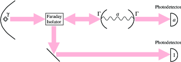
FIG. 1.: Diagram of the experimental configuration for obtaining the fluorescence of an atom as a beam, and passing it through a filter cavity.

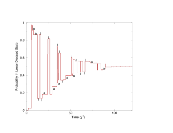
FIG. 2.: Probability for the atom to be in the dressed state $|{-}\rangle$ for a typical observation record from spectral detection using a single cavity tuned to the resonant frequency of the atom. The symbol a denotes the state following the detection of a photon at photodetector $a$ and l at photodetector $1$ (see Fig. 1). The parameters used are $\Omega/\gamma=50$, $\Gamma/\gamma=8$.

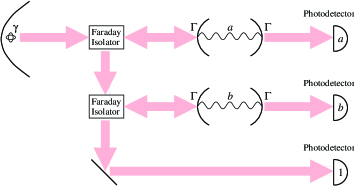
FIG. 3.: Diagram of the experimental configuration for passing the fluorescence of an atom through two filter cavities.

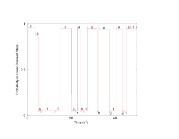
FIG. 4.: Probability for the atom to be in the dressed state $|{-}\rangle$ for spectral detection using two cavities tuned to the sidebands of the Mollow triplet, $\omega_{0}\pm\Omega$. The symbol a denotes the state following the detection of a photon at photodetector $a$, b at photodetector $b$, and l at photodetector $1$ (see Fig. 3). The parameters used are $\Omega/\gamma=50$, $\Gamma/\gamma=8$.

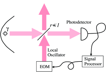
FIG. 5.: Diagram of the experimental configuration for a homodyne measurement of the fluorescence of an atom. The amplitude of the local oscillator is assumed to be variable as a function of time, determined by an electro-optic modulator (EOM). The modulator can be controlled by the experimenter using the results of the measurement.

FIG. 6.: Locus of various states of the Bloch sphere: $|{h}\rangle,|{l}\rangle$ from Sec. IV for $\Omega/\gamma\in[1/2,\infty)$ (solid line and circle); $|{\psi_{\rm s}^{\pm}}\rangle$ from Sec. V for $\Omega/\gamma\in[0,\infty)$ (dashed line and square); $|{\theta_{\pm}}\rangle$ from Sec. VI for $\Omega/\gamma\in[1,\infty)$ (solid line and cross). The circle, square and cross show the states for $\Omega=2\gamma$. Also shown are the dressed states $|{\pm}\rangle$ (asterisks) and the high-driving limit of the TM states $|{\phi_{1}}\rangle,|{\phi_{2}}\rangle$ (diamonds). An equal area projection of the sphere in terms of the Euler angles $\phi,\theta$ is used.

FIG. 7.: Stationary probability distribution of the atomic state on the Bloch sphere under the orthogonal jump detection scheme. The distribution is approximated by 1000 points, which are separated in time by 0.015 $\gamma^{-1}$. The ratio of driving to damping is $\Omega/\gamma=10$. The same equal area projection of the sphere as in Fig. 6 is used, but note that the $\phi$ axis is cut at a different point.

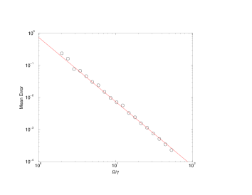
FIG. 8.: Mean error (ie. probability for the system not to be in the predicted dressed state) versus $\Omega/\gamma$ for orthogonal jump evolution. The fitted curve is $\epsilon_{\rm app}=2.99\times({\gamma}/{2\Omega})^{2}$

REFERENCES

- [1] N. Bohr, Phil. Mag. 26, 1 (1913).
- [2] W. Heisenberg, “Quantum Theory and its Interpretations” in S. Rozental (ed.), Neils Bohr: His life and works as seens by his friends and colleagues (North Holland, Amsterdam, 1967).
- [3] P.A.M. Dirac, The Principles of Quantum Mechanics (Oxford University Press, London, 1930).
- [4] V.F. Weisskopf and E.P. Wigner, Zeits. Phys. 63, 54 (1930).
- [5] F. Bloch, Phys. Rev. 70, 460 (1946).
- [6] R. Zwanzig, J. Chem Phys. 33, 1338 (1960).
- [7] W.H. Louisell, Quantum Statistical Properties of Radiation (John Wiley & Sons, New York, 1973).
- [8] C. Cohen-Tannoudji and S. Reynaud, Phil. Trans. R. Soc. Lond. A 293, 223 (1979).
- [9] B.R. Mollow, Phys. Rev. 188, 1969 (1969).
- [10] J.C. Bergquist et al., Phys. Rev. Lett. 57, 1699 (1986).
- [11] C. Cohen-Tannoudji and J. Dalibard, Europhys. Lett. 1, 441 (1986).
- [12] P. Zoller, M. Marte and D.F. Walls, Phys. Rev. A 35, 198 (1987).
- [13] H.J. Carmichael, S. Singh, R. Vyas, and P.R. Rice, Phys. Rev. A 39, 1200 (1989).
- [14] H.J. Carmichael, An Open Systems Approach to Quantum Optics (Springer-Verlag, Berlin, 1993).
- [15] C.W. Gardiner, A.S. Parkins, and P. Zoller, Phys. Rev. A 46, 4363 (1992).
- [16] H.M. Wiseman and G.J. Milburn, Phys. Rev. A 47, 642 (1993).
- [17] H.M. Wiseman and G.J. Milburn, Phys. Rev. Lett. 70, 548 (1993).
- [18] H.M. Wiseman and G.J. Milburn, Phys. Rev. A 47, 1652 (1993).
- [19] H.M. Wiseman, Phys. Rev. A 47, 5180 (1993).
- [20] H.M. Wiseman, Phys. Rev. A 49, 2133 (1994); Errata ibid., 49 5159 (1994) and ibid. 50, 4428 (1994).
- [21] H.J. Carmichael, Phys. Rev. Lett. 70, 2273 (1993).
- [22] H.J. Carmichael, P. Kochan, and L. Tian, in Proceedings of the International Symposium on Coherent States: Past, Present, and Future (World Scientific, Singapore, 1994).
- [23] B.M. Garraway and P.L. Knight, Phys. Rev. A 50, 2548 (1994).
- [24] P. Goetsch and R. Graham, Phys. Rev. A 50, 5242 (1994).
- [25] J. Dalibard, Y. Castin and K. Mølmer, Phys. Rev. Lett. 68, 580 (1992).
- [26] K. Mølmer, Y. Castin, and J. Dalibard, J. Opt. Soc. Am. B 10, 524 (1993).
- [27] R. Dum, P. Zoller and H. Ritsch, Phys. Rev. A 45, 4879 (1992).
- [28] P. Marte, R. Dum, R. Taïeb and P. Zoller, Phys. Rev. A 47, 1378 (1993).
- [29] P. Marte et al Phys. Rev. Lett. 71, 1335 (1993).
- [30] M. Holland, S. Marksteiner, P. Marte and P. Zoller, Phys. Rev. Lett. 76, 3683 (1996).
- [31] W.G. Teich and G. Mahler, Phys. Rev. A 45, 3300 (1992).
- [32] G. Lindblad, Commun. math. Phys. 48, 199 (1976).
- [33] C.W. Gardiner, Quantum Noise (Springer-Verlag, Berlin, 1991).
- [34] A.S. Holevo, Probabilistic and Statistical Aspects of Quantum Theory (North-Holland, Amsterdam, 1982).
- [35] M. Jack, M.J. Collett, and D.F. Walls, quant-ph/9807028, to be published in Phys. Rev. A.
- [36] D.T. Pegg and S.M. Barnett, unpublished (1999).
- [37] C.W. Gardiner, Phys. Rev. Lett. 70, 2269 (1993).
- [38] H.M. Wiseman, Phys. Rev. Lett. 75, 4587 (1995).
- [39] H.M. Wiseman, Quantum Semiclass. Opt 8, 205 (1996).
- [40] J.K. Breslin, G.J. Milburn, and H.M. Wiseman, Phys. Rev. Lett. 74, 4827 (1995).
- [41] L. Diósi, Phys. Lett. A 185, 5 (1994).
- [42] W.H. Zurek, Prog. Theor. Phys. 89, 281 (1993).
- [43] H.M. Wiseman and J.A. Vacarro, Phys. Lett. A 250, 241 (1998).