Quantum simulations of optical systems

Abstract

Within a framework of a two-dimensional microscopic purely-quantum mechanical model we analyze dynamics of single-photon wave packets interacting with optical elements (beam splitters, mirrors) modeled as systems of two-level atoms. That is, we utilize a two dimensional cavity to simulate the quantum behavior of simple optical components and networks thereof. The field is quantized using the canonical procedure, and only the basis states with one unit of excitation are included. This, however, covers the linear optical phenomena. The field is taken to interact with localized atoms through a dipole interaction. Using different configurations of atoms and choosing their frequencies to be resonant or off-resonance, we can model mirrors, beam splitters, focusing devices and multicomponent systems. Thus we can model arbitrary linear networks of optical components. We show the time evolution of a photon wave packet in an interferometer as an example. As the state of the field is known at each instant, spectral properties and spatial coherence can immediately be obtained from the simulations. We also know the states of the two level atoms constituting the components, which allows us to consider their quantum behavior. Here the decay of an excited atom into the vacuum state of the electromagnetic field in the two-dimensional cavity is studied.

I Introduction

It is well understood that the electromagnetic fields giving rise to all optical phenomena have ultimately to be represented by quantum operators. These couple to the degrees of freedom of matter and their modification due to this interaction constitutes the quantum counterpart of the action of optical components. Ordinary optical devices operate in the linear regime of interaction, but the important area of Nonlinear Optics is based on higher order effects of the field-matter coupling. In most situations, the optical phenomena can be described entirely in terms of classical fields, but many recent investigations require that the quantum character of the field is accounted for. Such research constitutes the topics of Quantum Optics [1, 2, 3]. However, many quantum effects are of interest even in the linear regime of operation: quantum noise [4] sets the limit to communication by optical channels and amplifiers, quantum interference shows up in precision measurements and tests of fundamental issues and also in reading and writing quantum information. Manipulation of quantum information such as quantum computations usually requires the inclusion of higher order effects, i.e. nonlinear interactions between the qubits [5].

In this paper, we are going to discuss the dynamics of single photon wave packets in various two-dimensional atomic configurations. These are taken to be models of optical networks, where we explicitly include the atomic nature of the optical components distributed over the volume under investigation. This approach provide us with a completely microscopic quantum-mechanical picture of how photon wave packets interact with optical elements represented as collections of two level atoms. For practical reasons, we have to restrict our work to one-photon states, but this is not such a serious limitation as it may seem. All linear optical effects are based on the single-photon interacting with material structures, and consequently we have a general description of Quantum Optics phenomena in the linear regime. The need to consider multi-photon effects arises only in connection with the quantum treatment of Nonlinear Optics.

There are two basic ways to approach the quantization of optical systems. In the conventional one, we determine a complete set of eigenmodes of the total universe, and express the fields of interest in terms of these. Any matter present is described through its interaction with the fields, and the coupled field-matter problem is then solved to the best of our ability. This is the approach utilized in traditional QED, and its development is found in many standard texts. The alternative approach, designed for Quantum Optics applications, is to determine the eigenmodes of the system at the classical level, the matter involved is then treated as boundary conditions on the field modes. Especially the new area of Cavity QED research [6], utilizes this point of view, and it provides the basis both for quantum communication theories and many fundamental investigations.

In the field of optics, the components are usually treated as boundary conditions only, and the complete optical device is considered to be an optical network. This approach has been discussed thoroughly in the classical regime of operation [7]. For linear devices, the classical treatment can be taken over into the quantum regime by the use of suitable Quantum Optics tools [8, 9, 10]. In principle, any device understood classically, can be treated quantum mechanically with such an approach. The specific quantum features manifest themselves in the initial conditions and the restrictions on observability imposed by quantum theory [11].

Another specifically quantum mechanical effect is the occurrence of spontaneous decay. Within a one-dimensional model of the modes of the universe, this is discussed in Ref. [12], where both free Weisskopf-Wigner decay and cavity modified decay are discussed. Such phenomena have been the object of much interest within QED research, for an extensive list of references see Ref. [12]. Within the model chosen there, one can see the emergence of the exponential law and the inhibition of decay observed in a photonic band gap structure. In general, the model provides insight into the role of atomic media in the irreversible transfer of excitation energy into the field modes of the universe.

In this paper we combine the two views discussed above: We retain a description in terms of a complete set of two-dimensional eigenmodes of the universe. The optical components are described in terms of their atomic constituents. All atomic structures are represented by spatially localized two-level atoms. These are treated as point-like partciles in accordance with the dipole approximation assumed to be valid. The state of the field is taken to be a single photon wave packet with a narrow energy distribution. In this case, the state can be described by a truncated expansion in terms of modes of the universe. The spatially distributed two-level atoms describing the structures are taken to be initially in their ground states. The atoms can be chosen to resonate with the central frequency of the photon wave packet or be well off resonance; various effects can be modeled in this way. When the single photon is absorbed, only one of the atoms is excited, and the field is reduced to its ground state. Such a choice limits the Hilbert space needed in the calculations to manageable size, but allows us to investigate many simple networks of significance in linear optics. All such effects are, in principle, describable at the single photon level; only Nonlinear Optics effects require more photons, which would make the Hilbert space expand beyond the limits of available computer resources.

Our approach based on a complete set of eigenmodes allows us to investigate the dynamic performance of many linear systems. In order to illustrate the method, we select the simplest optical components: mirrors, beam splitters, focusing devices and interferometers. The over-all performance of the components follows directly from their classical theory, but our approach allows us to investigate the microscopic (quantum) behavior of the setup. Quantum coherence between various spatial regions in the device is directly visible in the states calculated, and the time and space scales of the various interferometric structures can be read off the results. Combined with various models of measurements, our calculations contain considerably more information than a simple classical computation. Here we only discuss the measurement of frequency and the possible occurrence of filtering action in the atomic structures, which does not in itself depend too much on the quantum nature of the fields. But modeling the frequency detection by atomic absorption, we utilize the full character of the model, which allows further extension to quantum correlation measurements if we so desire.

Our work is based on the model put forward in [13] which we extend to two dimensions. The quantized modes of the universe are introduced in Sec. II together with their interaction with the spatially distributed atoms. In Sec. III we specify the details of the model and indicate how the calculations have been carried out. Section IV presents the various simple components analyzed in this paper. We describe how they are modeled and show the results of the detailed solution of the time evolution. Finally in Sec. V we present our conclusions and discuss possible extensions and applications of the work.

II Operators for the free field in two dimensions

The field is enclosed inside a two dimensional cavity determined by the relations

$$-\frac{L}{2}\leq x,y\leq\frac{L}{2}.$$ (1)

The periodic boundary conditions restrict the allowed values in ${\bf k}$-space to a discrete set

$$k_{i}=\frac{2\pi n_{i}}{L},\ \ \ i=x,y.$$ (2)

In computer simulations, the ${\bf k}$-values must be restricted by giving some upper limit for the integer $n$ which corresponds to a specific frequency cut-off. The electric and magnetic field can be expanded [3] using the mode functions

$$\hat{\bf E}({\bf r})=\frac{i}{L}\sum_{{\bf k}s}\left(\frac{\hbar\omega_{{\bf k}s}}{2\epsilon_{0}}\right)^{1/2}(\hat{a}_{{\bf k}s}{\bf\epsilon}_{{\bf k}s}e^{i{\bf k}\cdot{\bf r}}-{\rm h.c})$$ (3)

$$\hat{\bf B}({\bf r})=\frac{i}{L}\sum_{{\bf k}s}\left(\frac{\hbar}{2\epsilon_{0}\omega_{{\bf k}s}}\right)^{1/2}(\hat{a}_{{\bf k}s}({\bf k}\times{\bf\epsilon}_{{\bf k}s})e^{i{\bf k}\cdot{\bf r}}-{\rm h.c}),$$ (4)

where the summation $\sum\limits_{{\bf k}s}$ is over all ${\bf k}$-values (2) and two polarization indices $s=1,2$. The frequency $\omega_{{\bf k}s}$ is the same for both polarizations

$$\omega_{{\bf k}s}=c|{\bf k}|.$$ (5)

The general k-vector in two dimensions can be written

$${\bf k}=k_{x}\hat{e}_{1}+k_{y}\hat{e}_{2}=|{\bf k}|(\cos(\phi)\hat{e}_{1}+\sin(\phi)\hat{e}_{2}).$$ (6)

The polarization vectors which obey the usual right hand rule conventions are

$${\bf\epsilon}_{{\bf k}1}=-\hat{e}_{3}$$ (7)

$${\bf\epsilon}_{{\bf k}2}=-\sin(\phi)\hat{e}_{1}+\cos(\phi)\hat{e}_{2}.$$ (8)

The ${\bf k}$-vector and polarization indexes satisfy the relations [3]

$${\bf\epsilon}_{{\bf k}i}\cdot{\bf\epsilon}_{{\bf k}j}=\delta_{ij}$$ (9)

$$\sum\limits_{ss^{\prime}}{\bf\epsilon}_{{\bf k}s}\cdot{\bf\epsilon}_{{\bf k}s^{\prime}}=2$$ (10)

$${\bf k}\times{\bf\epsilon}_{{\bf k}1}=-k_{y}\hat{e}_{1}+k_{x}\hat{e}_{2}$$ (11)

$${\bf k}\times{\bf\epsilon}_{{\bf k}2}=|{\bf k}|\hat{e}_{3}.$$ (12)

The energy-density operator is

$$\hat{H}({\bf r})=\frac{1}{2}\epsilon_{0}\hat{{\bf E}}^{2}({\bf r})+\frac{1}{2\mu_{0}}\hat{{\bf B}}^{2}({\bf r})$$ (13)

Using (3) and (4) gives

$$\frac{1}{2}\epsilon_{0}{\bf\hat{E}}^{2}({\bf r}) = -\frac{\hbar}{4L^{2}}\sum\limits_{{\bf k}{\bf k}^{\prime}ss^{\prime}}\sqrt{\omega_{\bf k}\omega_{{\bf k}^{\prime}}}\big{(}\hat{a}_{{\bf k}s}\hat{a}_{{\bf k}^{\prime}s^{\prime}}e^{i{\bf k}\cdot{\bf r}+i{\bf k}^{\prime}\cdot{\bf r}}-\hat{a}_{{\bf k}s}\hat{a}_{{\bf k}^{\prime}s^{\prime}}^{{\dagger}}e^{i{\bf k}\cdot{\bf r}-i{\bf k}^{\prime}\cdot{\bf r}}$$ (15)

$$\hskip 142.26378pt-\hat{a}_{{\bf k}s}^{{\dagger}}\hat{a}_{{\bf k}^{\prime}s^{\prime}}e^{-i{\bf k}\cdot{\bf r}+i{\bf k}^{\prime}\cdot{\bf r}}+\hat{a}_{{\bf k}s}^{{\dagger}}\hat{a}_{{\bf k}^{\prime}s^{\prime}}^{{\dagger}}e^{-i{\bf k}\cdot{\bf r}-i{\bf k}^{\prime}\cdot{\bf r}}\big{)}$$

$$\frac{1}{2\mu_{0}}{\bf\hat{B}}^{2}({\bf r}) = -\frac{\hbar}{4L^{2}\mu_{0}\epsilon_{0}}\sum\limits_{{\bf k}{\bf k}^{\prime}ss^{\prime}}\frac{1}{\sqrt{\omega_{\bf k}\omega_{{\bf k}^{\prime}}}}(\hat{a}_{{\bf k}s}\hat{a}_{{\bf k}^{\prime}s^{\prime}}e^{i{\bf k}\cdot{\bf r}+i{\bf k}^{\prime}\cdot{\bf r}}-\hat{a}_{{\bf k}s}\hat{a}_{{\bf k}^{\prime}s^{\prime}}^{{\dagger}}e^{i{\bf k}\cdot{\bf r}-i{\bf k}^{\prime}\cdot{\bf r}}$$ (17)

$$-\hat{a}_{{\bf k}s}^{{\dagger}}\hat{a}_{{\bf k}^{\prime}s^{\prime}}e^{-i{\bf k}\cdot{\bf r}+i{\bf k}^{\prime}\cdot{\bf r}}+\hat{a}_{{\bf k}s}^{{\dagger}}\hat{a}_{{\bf k}^{\prime}s^{\prime}}^{{\dagger}}e^{-i{\bf k}\cdot{\bf r}-i{\bf k}^{\prime}\cdot{\bf r}})[(k_{x}k_{x}^{\prime}+k_{y}k_{y}^{\prime})\delta_{s1}\delta_{s^{\prime}1}+|{\bf k}||{\bf k}^{\prime}|\delta_{s2}\delta_{s^{\prime}2}]$$

In our simulations, we have restricted the polarization of the field to ${\bf\epsilon}_{{\bf k}1}$. The modes with $s=2$ are taken to have have zero amplitudes. In addition to that we restrict the number of excitations of our basis vectors to one. For these kind of basis vectors the terms $\hat{a}_{{\bf k}s}\hat{a}_{{\bf k}^{\prime}s^{\prime}}$ and $\hat{a}_{{\bf k}s}^{{\dagger}}\hat{a}_{{\bf k}^{\prime}s^{\prime}}^{{\dagger}}$ do not give any contribution. These terms can be omitted from the expressions. For the states described above, the expectation values are obtained by replacing the operators with the coefficients of the corresponding statevectors $\hat{a}_{\bf k}\rightarrow c_{\bf k}$ and $\hat{a}_{\bf k}^{{\dagger}}\rightarrow c_{\bf k}^{*}$. The normally-ordered terms in the energy density become (normal ordering is indicated by colons)

$$:\frac{1}{2}\epsilon_{0}{\bf\hat{E}}^{2}({\bf r}): = \frac{\hbar}{2L^{2}}RR^{*}$$ (18)

$$:\frac{1}{2\mu_{0}}{\bf\hat{B}}^{2}({\bf r}): = \frac{\hbar}{2L^{2}\epsilon_{0}\mu_{0}}(S_{x}S_{x}^{*}+S_{y}S_{y}^{*}),$$ (19)

where

$$R = \sum\limits_{\bf k}\sqrt{\omega_{\bf k}}c_{\bf k}e^{i{\bf k}\cdot{\bf r}}$$ (20)

$$S_{i} = \sum\limits_{\bf k}\frac{k_{i}}{\sqrt{\omega_{\bf k}}}c_{\bf k}e^{i{\bf k}\cdot{\bf r}},\ \ \ i=x,y.$$ (21)

The two-fold summation over the ${\bf k}$-space is seen to factorize and the formulas for $R$ and $S_{i}$ are Fourier transforms of two different functions. For numerical simulations these two properties are essential as will be seen later. We note that if the polarization is such that the modes with $s=1$ are taken to have zero amplitudes, then the two terms $:\frac{1}{2}\epsilon_{0}{\bf\hat{E}}^{2}({\bf r}):$ and $:\frac{1}{2\mu_{0}}{\bf\hat{B}}^{2}({\bf r}):$ in the expression for the energy density are equal.

Integrating (13) over the spatial coordinates and using the integral

$$\int\limits_{-L/2}^{L/2}dx\int\limits_{L/2}^{L/2}dye^{i({\bf k}-{\bf k}^{\prime})\cdot{\bf r}}=L^{2}\delta_{{\bf k}{\bf k}^{\prime}}$$ (22)

gives the familiar form

$$\hat{H}_{F}=\frac{1}{2}\sum\limits_{{\bf k}}\hbar\omega_{{\bf k}}(\hat{a}_{{\bf k}}^{{\dagger}}\hat{a}_{{\bf k}}+\hat{a}_{{\bf k}}\hat{a}_{{\bf k}}^{{\dagger}})=\sum_{{\bf k}}\hbar\omega_{\bf k}(\hat{a}_{{\bf k}}^{{\dagger}}\hat{a}_{{\bf k}}+\frac{1}{2}),$$ (23)

which in the normally ordered form reads $:\hat{H}_{F}:=\sum\limits_{{\bf k}}\hbar\omega_{\bf k}\hat{a}_{{\bf k}}^{{\dagger}}\hat{a}_{{\bf k}}$

III The General Hamiltonian and the states

In the previous chapter the formulas for the field in the vacuum were derived. In this chapter we add an assembly of two level atoms to the cavity and give the corresponding Hamiltonians. The general form of the statevector with one excitation is also given. The material presented here is based on the similar simulations in one dimension done by V.Bužek et.al. [12]. The simulations in two dimensions are numerically more demanding, but we have been able to develop efficient numerical methods which make these simulations possible.

A The Hamiltonian

The total Hamiltonian $\hat{H}$ can be divided into three parts

$$\hat{H}=\hat{H}_{F}+\hat{H}_{A}+\hat{H}_{I},$$ (24)

where the field Hamiltonian is given by equation (23). The atomic Hamiltonian is the sum over all one-atom Hamiltonians

$$\hat{H}_{A}=\sum\limits_{j=1}^{N_{A}}\hbar\omega_{j}\hat{\sigma}_{z}^{j}$$ (25)

where $\omega_{j}$ is the transition frequency of the $j$-th atom and $\hat{\sigma}_{z}^{j}$ is Pauli’s spin matrix. In the interaction Hamiltonian the dipole approximation is used. For simplicity the dipole operator is taken to be

$${\bf\hat{D}}_{j}=(D_{j}\hat{\sigma}_{+}^{j}+D_{j}^{*}\hat{\sigma}_{-}^{j})\hat{e}_{3},$$ (26)

i.e. it has a component in the $\hat{e}_{3}$ direction only. The general dipole vector would have components in the $x$- and $y$-directions too. The interaction Hamiltonian has the form

$$H_{I}=-\sum\limits_{j=1}^{N_{A}}\hat{\bf D}_{j}\cdot\hat{\bf E}({\bf r}_{j}),$$ (27)

where $\hat{\bf E}({\bf r}_{j})$ is the electric field operator (3) at the position of the atom. The rotating wave approximation (RWA) is to be used, and we neglect the $\hat{\sigma}+^{j}\hat{a}^{{\dagger}}$ - and $\hat{\sigma}_{-}^{j}\hat{a}$ terms. In addition to that we replace the mode frequency in the electric field operator by the atomic frequency and use the dot products $\hat{e}_{3}\cdot{\bf\epsilon}_{{\bf k}1}=-1$ and $\hat{e}_{3}\cdot{\bf\epsilon}_{{\bf k}2}=0$ to get

$$\hat{H}_{I}\equiv\hat{H}_{I1}+\hat{H}_{I2}=\sum\limits_{j=1}^{N_{A}}\sum\limits_{{\bf k}}\left(g(j,{\bf k})\hat{\sigma}_{+}^{j}\hat{a}_{{\bf k}}g^{*}(j,{\bf k})\hat{\sigma}_{-}^{j}\hat{a}_{{\bf k}}^{{\dagger}}\right),$$ (28)

in what follows we omit the polarization index in subscripts of field operators. The coupling constant is

$$g(j,{\bf k})=-\frac{i\hbar}{2\epsilon_{0}L}\sqrt{\omega_{\bf k}}D_{j}e^{i{\bf k}\cdot{\bf r}_{j}}.$$ (29)

Only those modes whose resonance frequency is close to the atomic frequency interact significantly with the atom, so we can replace the mode frequency $\omega_{\bf k}$ by the atomic frequency $\omega_{j}$ in equation (29).

B The statevector

In all simulations we have restricted the total number of excitations to one. Consequently, the most general statevector of the atom-field system has the form

$$|\Psi\rangle = \sum\limits_{\bf k}\left(c_{\bf k}|1\rangle_{\bf k}\prod\limits_{{{\bf k}^{\prime}}\neq{\bf k}}\right)|0\rangle_{{\bf k}^{\prime}}\otimes\prod\limits_{j=1}^{N_{A}}|0\rangle_{j}$$ (31)

$$+\sum\limits_{\bf k}|0\rangle_{\bf k}\otimes\sum\limits_{j=1}^{N_{A}}\left(c_{j}|1\rangle_{j}\prod\limits_{j^{\prime}=1,j^{\prime}\neq j}^{N_{A}}|0\rangle_{j^{\prime}}\right)$$

$$\equiv \sum\limits_{\bf k}c_{\bf k}|1_{\bf k},\{0\}\rangle+\sum\limits_{j=1}^{N_{A}}c_{j}|\{0\},1_{j}\rangle.$$ (32)

The first sum contains all the basis vectors where the excitation is in one of the field modes and all the atoms are in the ground state. In the second sum the field modes are in the vacuum state and one of the atoms is excited. The complex numbers $c_{\bf k}$ and $c_{j}$ are the probability amplitudes of the corresponding basis vectors. We have dropped the polarization indices because in our simulations only the basis vectors with the polarization vector ${\bf\epsilon}_{{\bf k}1}$ are excited as was discussed earlier.

The general Gaussian one photon statevector is of the form

$$|\Psi\rangle=\sum\limits_{\bf k}c_{\bf k}|1_{\bf k},\{0\}\rangle,$$ (33)

where the mode coefficient $c_{\bf k}$ is

$$c_{\bf k}=\frac{e^{i{\bf k}\cdot{\bf r}_{0}}}{\sqrt{4\pi^{2}M}}\exp\big{(}-\frac{\Delta_{ky}^{2}}{4M}(k_{x}-k_{x0})^{2}$$ (35)

$$-\frac{\Delta_{kx}^{2}}{4M}(k_{y}-k_{y0})^{2}+\frac{\Delta_{kx,ky}^{2}}{2M}(k_{x}-k_{x0})(k_{y}-k_{y0})\big{)}.$$

The parameters $M$ and $\Delta_{kx,ky}^{2}$ are

$$M = \Delta_{kx}^{2}\Delta_{ky}^{2}-(\Delta_{kx,ky}^{2})^{2}$$ (36)

$$\Delta_{kx,ky}^{2} = \langle k_{x}k_{y}\rangle-\langle k_{x}\rangle\langle k_{y}\rangle.$$ (37)

If the cross-variance $\Delta_{kx,ky}^{2}$ vanishes the formula for $c_{\bf k}$ reduces to two independent Gaussian distributions

$$c_{\bf k}=(2\pi\Delta_{kx}^{2})^{-1/4}(2\pi\Delta_{ky}^{2})^{-1/4}e^{-i{\bf k}\cdot{\bf r}_{0}}$$ (39)

$$\exp\left[-\frac{(k_{x}-k_{x0})^{2}}{4\Delta_{kx}^{2}}-\frac{(k_{y}-k_{y0})^{2}}{4\Delta_{ky}^{2}}\right]$$

All initial distributions used in our simulations are of the form (39). The distribution (39) in ${\bf k}$-space is centered around $(k_{x0},k_{y0})$ with the corresponding central frequency $\omega_{0}$. If $\Delta_{kx}^{2}=\Delta_{ky}^{2}$ the distribution is symmetric. If $\Delta_{kx}^{2}<\Delta_{ky}^{2}$ the distribution is wider in the $y$-direction (and vice versa). The variances in ${\bf k}$-space and configuration space are inversely proportional. If $\Delta_{kx}^{2}$ is small, the energy density distribution in configuration space is wide in the x-direction. The normally ordered energy distribution associated with the state (35) or (39) is well localized near the point ${\bf r}_{0}$ in the configuration space. Essential for this is the phase part $e^{-i{\bf k}\cdot{\bf r}_{0}}$ of the coefficient $c_{\bf k}$. If the form of the phase was different the intensity profile would not be Gaussian.

The time evolution of the Gaussian wave packet inside an empty cavity is determined by the Hamiltonian $\hat{H}_{F}$ (23) with the corresponding evolution operator $\exp(-\frac{i}{\hbar}\hat{H}_{F}t)$. Applying this to the state (31) gives for the time-evolution of the coefficients $c_{\bf k}(t)=c_{\bf k}(0)e^{-i\omega_{\bf k}t}$. The absolute value of the coefficients remain the same, only the phase changes. For the phase part we get

$$\exp(-i{\bf k}\cdot{\bf r}_{0}-i\omega_{\bf k}t)=\exp[-i{\bf k}\cdot({\bf r}_{0}+ct{\bf e}_{\bf k})],$$ (40)

where ${\bf k}=|{\bf k}|{\bf e}_{\bf k}$. The time evolution inside the empty cavity reduces to the time evolution of the parameter ${\bf r}(t)={\bf r}_{0}+ct{\bf e}_{\bf k}$. We remember that the phase factor determine the shape of the normal ordered intensity profile. Because the time evolution of the phase is different for different modes, the normal ordered intensity does not preserve its original Gaussian shape. If the direction of the vector ${\bf e}_{\bf k}$ is more or less the same for all basis vectors which have nonzero coefficients, the shape of the energy density distribution remains approximately the same longer. The situation is like this when the state vector in ${\bf k}$-space is centered around some ${\bf k}$-value far from the origin and the variances are small.

C Transformation to the interaction picture

It turned out to be faster to carry out the numerical integration in the interaction picture. The transformation Hamiltonian is $\hat{H}_{0}=\hat{H}_{A}+\hat{H}_{F}$. The interaction Hamiltonian in the rotating frame is

$$\hat{H}_{I}^{(I)}=\exp(i\hat{H}_{0}t/\hbar)\hat{H}_{I}\exp(-i\hat{H}_{0}t/\hbar),$$ (41)

which is obtained by the following replacement

$$\hat{a}_{\bf k} \rightarrow \hat{a}_{\bf k}e^{-i\omega_{\bf k}t}$$ (42)

$$\hat{a}_{\bf k}^{{\dagger}} \rightarrow \hat{a}_{\bf k}^{{\dagger}}e^{i\omega_{\bf k}t}$$ (43)

$$\hat{\sigma}_{-}^{j} \rightarrow \hat{\sigma}_{-}^{j}e^{-i\omega_{j}t}$$ (44)

$$\hat{\sigma}_{+}^{j} \rightarrow \hat{\sigma}_{+}^{j}e^{i\omega_{j}t}$$ (45)

in equation (28), and we get

$$\hat{H}_{I}^{(I)} = \hat{H}_{I1}^{(I)}+\hat{H}_{I2}^{(I)}$$ (46)

$$= \sum\limits_{j=1}^{N_{A}}\sum_{\bf k}\big{(}g(j,{\bf k})e^{i(\omega_{j}-\omega_{\bf k})t}\hat{\sigma}_{+}^{j}\hat{a}_{\bf k}$$ (48)

$$\hskip 28.45274pt+g^{*}(j,{\bf k})e^{-i(\omega_{j}-\omega_{\bf k})t}\hat{\sigma}_{-}^{j}\hat{a}_{\bf k}^{{\dagger}}\big{)}.$$

The statevectors in the interaction picture become

$$|\Psi\rangle^{(I)} = \exp(i\hat{H}_{0}t/\hbar)|\Psi\rangle$$ (49)

$$= \sum\limits_{\bf k}c_{\bf k}e^{i\omega_{\bf k}t}|1_{\bf k},\{0\}\rangle+\sum\limits_{j=1}^{N_{A}}c_{j}e^{i\omega_{j}t}|\{0\},1_{j}\rangle.$$ (50)

and the Schrödinger equation for the wavefunction is

$$i\hbar\frac{d|\Psi\rangle^{(I)}}{dt}=\hat{H}_{I}^{(I)}|\Psi\rangle^{(I)}.$$ (51)

Integration of the Schrödinger equation in the interaction picture is faster than the original equation because only the interaction Hamiltonian is present.

D Numerical methods

1 Integration of Schrödinger equation

Our choice for the integration method of the time dependent Schrödinger equation is a classical four stage fourth order Runge-Kutta method. If the wavefunction at time $t$ is $|\Psi(t)\rangle$ the wavefunction at a later time $t+\Delta t$ ($\Delta t$ small) $|\Psi(t)\rangle$ is given by the following algorithm [14]

$$|k_{1}\rangle = \Delta t\hat{H}|\Psi(t)\rangle$$ (52)

$$|k_{2}\rangle = \Delta t\hat{H}(|\Psi(t)\rangle+0.5|k_{1}\rangle)$$ (53)

$$|k_{3}\rangle = \Delta t\hat{H}(|\Psi(t)\rangle+0.5|k_{2}\rangle)$$ (54)

$$|k_{4}\rangle = \Delta t\hat{H}(|\Psi(t)\rangle+0.5|k_{3}\rangle)$$ (55)

$$|\Psi(t+\Delta t)\rangle = |\Psi(t)\rangle+\frac{|k_{1}\rangle}{6}+\frac{|k_{2}\rangle}{3}+\frac{|k_{3}\rangle}{3}+\frac{|k_{4}\rangle}{6}+O((\Delta t)^{5}).$$ (56)

The timestep $\Delta t$ is a fixed constant.

The essential part of the integration from the numerical point of view is how to evaluate the right hand part of the equation (51) as efficiently as possible. The first term in the equation (46) gives

$$\hat{H}_{I1}|1_{\bf k},\{0\}\rangle=$$ (60)

$$-\frac{i\hbar}{2\epsilon_{0}L}\sum\limits_{j=1}^{N_{A}}\sum\limits_{\bf k^{\prime}}\sqrt{\omega_{j}}D_{j}\exp(i{\bf k^{\prime}}\cdot{\bf r}_{j})e^{i(\omega_{j}-\omega_{\bf k})t}\sigma_{+}^{j}\hat{a}_{{\bf k^{\prime}}1}|1_{\bf k},\{0\}\rangle$$

$$=-\frac{i\hbar}{2\epsilon_{0}L}\sum\limits_{j=1}^{N_{A}}\sqrt{\omega_{j}}D_{j}\exp(i{\bf k}\cdot{\bf r}_{j})e^{i(\omega_{j}-\omega_{\bf k})t}|\{0\},1_{j}\rangle$$

$$\hat{H}_{I1}|\{0\},1_{j}\rangle=0,$$

and the second one

$$\hat{H}_{I2}|1_{\bf k},\{0\}\rangle=0$$ (61)

$$\hat{H}_{I2}|\{0\},1_{j}\rangle=$$ (64)

$$\frac{i\hbar}{2\epsilon_{0}L}\sum\limits_{j=1}^{N_{A}}\sum\limits_{\bf k}\sqrt{\omega_{j}}D_{j}^{*}\exp(-i{\bf k}\cdot{\bf r}_{j})e^{-i(\omega_{j}-\omega_{\bf k})t}\sigma_{-}^{j}\hat{a}_{{\bf k}1}^{{\dagger}}|\{0\},1_{j}\rangle$$

$$=\frac{i\hbar}{2\epsilon_{0}L}\sum\limits_{\bf k}\sqrt{\omega_{j}}D_{j}^{*}\exp(-i{\bf k}\cdot{\bf r}_{j})e^{-i(\omega_{j}-\omega_{\bf k})t}|1_{\bf k},0\rangle.$$

Hence the new coefficients for the atomic ($c_{j}^{\prime}$) and field ($c_{\bf k}^{\prime}$) basis vectors become

$$c_{j}^{\prime} = -\frac{i\hbar}{2\epsilon_{0}L}\sqrt{\omega_{j}}D_{j}e^{i\omega_{j}t}T({\bf r}_{j},t)$$ (65)

$$c_{\bf k}^{\prime} = \frac{i\hbar}{2\epsilon_{0}L}e^{i\omega_{\bf k}t}U({\bf k},t),$$ (66)

where

$$T({\bf r},t)=\sum\limits_{\bf k}\left(c_{\bf k}e^{-i\omega_{\bf k}t}\right)e^{i{\bf k}\cdot{\bf r}}$$ (67)

$$U({\bf k},t)=$$ (69)

$$\sum\limits_{\bf r}\left(\sum\limits_{j=1}^{N_{A}}\sqrt{\omega_{j}}D_{j}^{*}c_{j}\delta({\bf r}-{\bf r}_{j})e^{-i\omega_{j}t}\right)e^{-i{\bf k}\cdot{\bf r}}.$$

Both $T({\bf r},t)$ and $U({\bf k},t)$ are two dimensional Fourier transforms, so in numerical calculations the Fast Fourier Transform (FFT) can be used. The speed increase obtained by using FFT instead of the direct summation is enormous especially in simulations with a large number of atoms. In some simulations it can be said that only this method makes these simulations possible.

There are several natural checks for the numerical simulations. First of all the norm of the wavefunction has to remain unity for all times. The system is closed so the total energy of the system must be constant all the time. The field energy can be calculated using either the formula (23) or integrating the energy density over the whole cavity. The two methods should give the same results.

2 A method to detect a local time dependent spectrum

In the following simulations the spectrum is detected using so-called analyzer atoms [15]. Many atoms with a very small dipole coupling constant are put into specific locations in the cavity. All the atoms have different transition frequencies in between $\omega_{min}$ and $\omega_{max}$

$$\omega_{j}=\omega_{min}+\Delta\omega\cdot(j-1) \ \ \Delta\omega=\frac{\omega_{max}-\omega_{min}}{N-1},$$ , (71)

$$j=1,2...N$$

Also the dipole constants are all different and very small

$$D_{j}=\frac{C}{\omega_{j}},$$ (72)

where $C$ is a very small constant, typically C=0.0001 or so. The form (72) of $D_{j}$ gives the same decay constant $\Gamma$ for all the atoms because in two dimensions $\Gamma$ is directly proportional to the product $D_{j}^{2}\omega_{j}^{2}$. Because the dipole coupling is small, the atoms have very small decay constants and linewidths and only the radiation which is exactly on resonance with the atom can excite it. Therefore the excitation of the atoms as function of $\omega$ can be interpreted as a spectrum of the field at the position of the atoms. Because the interaction between the radiation and the atoms is small, the state of the field does not change appreciably. The method can be used to detect the local time dependent spectrum. Two-time averages, usually used in spectrum calculations, are not needed. A more detailed description of the method and comparisons with the time dependent spectra defined using two-time averages [16] can be found in the paper by M.Havukainen and S.Stenholm [15], where it was used to detect the spectrum of a radiation emitted by a laser driven three level atom.

IV Simulations

In this chapter the results of several simulations are presented. First we show that the energy density profile of the free photon does not preserve its shape if $\omega_{0}$ is small as was explained earlier. In the second and third simulation, atoms are used as mirrors and beam splitters. Using these components it is possible to build many optical systems. We present an interferometer as an example. We also present a simulation of a two-slit experiment. Finaly, we also briefly study a spontaneous decay of a two level atom into the vacuum of electromagnetic modes in the two-dimensional cavity.

A A free photon

In the first simulation the time evolution of the free photon wave packet is studied. The initial wave packet is Gaussian (39) with parameters $x_{0}=-8.0$, $y_{0}=0.0$, $k_{x0}=4.0$, $k_{y0}=0.0$ and $\Delta_{kx}^{2}=\Delta_{ky}^{2}=1.0$. The probabilities $|c_{\bf k}|^{2}$ of the field modes are shown Fig. 1. The central frequency of the photon wave packet is so small that the ${\bf k}$-vectors of the modes with nonzero amplitudes are not parallel. We would expect this to be observed as was explained earlier. The time evolution of the energy density at two time values is shown in Fig. 2. The initial Gaussian photon wave packet has an energy density centered at $x=-8.0$, $y=0.0$. The wave packet is moving to the right. During the free evolution energy density becomes delocalized. From the figure we see that at $t=20.0$ the width in the $y$-direction is much larger than the initial value. This spread of the width of the original wave packet is a standard quantum-mechanical effect.

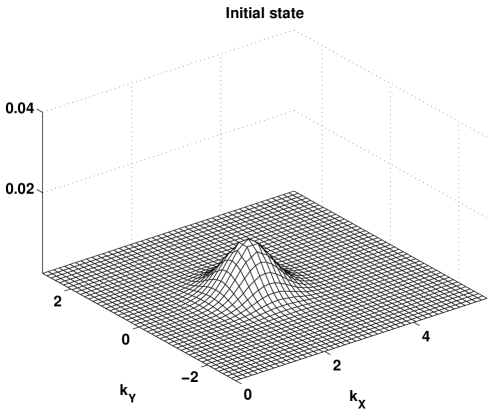
FIG. 1.: The probabilities $|c_{\bf k}|^{2}$ of the Gaussian initial state in ${\bf k}$-space. The parameters in the equation (39) are $x_{0}=-8.0$, $y_{0}=0.0$, $k_{x0}=4.0$, $k_{y0}=0.0$, $\Delta_{kx}^{2}=1.0$ and $\Delta_{ky}^{2}=1.0$. Here we consider the size of the cavity to be $L=10\pi$ and we take into account $256\times 256$ modes of the electromagnetic field. Only one polarization ($s=1$) is taken into account.

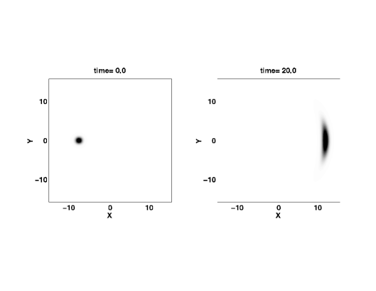
FIG. 2.: The time evolution of the energy density of of the initial Gaussian photon in free space. The parameters are the same as in Fig. 1. We see that the initial wave packet (a) is nicely localized in the configuration space while at later times it does not preserve its initial shape - we see (b) the spreading of the original wave packet in the $y$-direction.

B A mirror

It is possible to “build” mirrors and beam splitters using two level atoms. In the next simulation many atoms with large dipole constants were arranged into a slab configuration. We take a $45^{o}$ angle between the slab and the $x$-axis. We assume all atoms to have the same transition frequencies and dipole constants. The initial photon wave packet has a Gaussian distribution (39) with parameters $k_{x0}=5.0$, $k_{y0}=0.0$ and $\Delta_{kx}^{2}=\Delta_{ky}^{2}=0.125$. The atoms in the slab are exactly on resonance with the incoming photon wave packet (i.e. the central frequency of the wave packet $\omega_{0}=5.0$ is equal to the transition frequency of the atoms). The dipole constant is large $D=0.5$. We assume that the mirror is composed of eight layers of atoms as close to each other as possible. In our case we assume to distance between neighboring layers of the atoms to coincide with the grid in the configuration space (the grid spacing is $\Delta x$ and for the given orientation of the mirror the distance between the different atomic layers is chosen to be $\Delta X=\sqrt{2}\cdot\Delta x=0.17$). The central wavelength of the incoming photon wave packet is $\lambda=1.26$ so the difference between the neighboring atoms much shorter than the wavelength of the incoming wave packet.

We plot the energy density of the one-photon wave packet reflected by the mirror in Fig. 3. Firstly we plot the initial wave packet at $t=0.0$ (a). The photon is coming towards the atoms of the mirror. These atoms become excited by the incoming wave packet. The “secondary” radiation which is emitted by the atoms interfere with the incoming wave packet. This secondary radiation can formally be expressed as a sum of the two terms - the first destructively interfere with the incoming wave packet. As a consequence of this interference the incoming wave packet is “destroyed” (i.e. becomes extinct). The other part of the radiation which is “collectively” radiated by the atoms of the mirror represents the reflected wave packet. In fact, the process of reflection of the wave packet by atoms of the mirror represents purely quantum (microscopic) version of the Ewald-Oseen extinction theorem [17]. In Fig. 3(b) we have chosen conditions such that at $t=20.0$ all the radiation is reflected by the atoms.

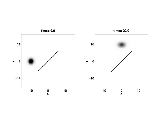
FIG. 3.: The energy density of the one-photon wave packet reflected by a mirror composed of two-level atoms. The initial photon is Gaussian (39) with parameters $x_{0}=-8.0$, $y_{0}=0.0$, $k_{x0}=5.0$, $k_{y0}=0.0$, $\Delta_{kx}^{2}=0.125$ and $\Delta_{ky}^{2}=0.125$. The atoms of the mirror are exactly on resonance with the central frequency of the photon wave packet ($\omega=5.0$). The dipole constant of the atom is chosen to be $D=0.5$. The total number of atoms considered in this simulation was 1584. The number of modes is the same as in the simulation presented in Fig. 2.

The direction of propagation of the reflected wave packet is the same as expected in the classical theory. The energy density compared to the incoming wave packet is changed but is still clearly localized. Note that the energy density is not perfectly symmetrical. The reason is the same as in the simulation with a free photon, i.e. the distribution in $k$-space is broad and near the origin so the spread of the wave packet is clearly seen. Additionally, the interference between components of radiation emitted by different atoms of the mirror plays a role. In the left part of Fig. 5 we see the energy density of the photon wave packet close to the surface of the mirror. We see that the incoming and reflected parts interfere. We also see that no energy is transmitted by the atomic slab. In this sense the atoms serve as a mirror. Nevertheless, one has to remember that the atoms during the process of reflection of the original wave packet become excited, that is the mirror under consideration has its own “internal” (quantum) degrees of freedom, so the part of the original energy can be (transiently) absorbed by the mirror. This also result in the fact that this quantum mirror might become entangled with the reflected wave packet.

We note that the parameters of the atoms in this simulation were carefully chosen in such a way that the atoms really form a mirror. If the parameters are changed then part of the radiation can be transmitted, that is the collection of the atoms can play a rôle of a beam splitter.

C A beam splitter

In the previous simulation we have shown that it is possible to build an almost perfect mirror using two level atoms, assuming the parameters are chosen correctly. Using slightly different parameters, we find that the atoms can behave as a beam splitter. There are several ways how to modify the “mirror” configuration to obtain a beam splitter – for instance, we can consider a smaller number of atoms, or we can decrease the dipole constants, or change the resonance frequencies of the atoms. We tried all the possibilities and the most satisfactory results were obtained by detuning the atoms. The frequencies of the atoms are now taken to be $\omega=10.4$. The center frequency of the incoming photon wave packet is $\omega_{0}=15.0$, i.e. the detuning is really large. The time evolution of the energy density of the electromagnetic field in this case is shown in Fig. 4. The line in the middle represents the positions of the detuned atoms. There is only one layer of atoms instead of eight as in the mirror simulation. At $t=0.0$ the photon is propagating towards the atoms. Here again the incoming wave packet excites the atoms. Now the quantum interference between the incoming and emitted radiation is such that part of the original wave packet is transmitted by the layer of the atoms. The other part is reflected. In Fig. 4 we clearly see that at $t=20.0$ the original wave packet is split into two parts propagating up and to the right. The energy is divided equally, that is the atoms form a 50-50 beam splitter for the incoming photon. Here we stress that the beam splitter under consideration has its own internal degrees of freedom and transiently it becomes excited. Nevertheless, after a while the atoms completely emit the excitation energy and the beam splitter is in a ground state - at this point it is completely disentangled from the one-photon radiation field which is now in a pure superposition state with two macroscopically distinguishable components (reflected and transmitted).

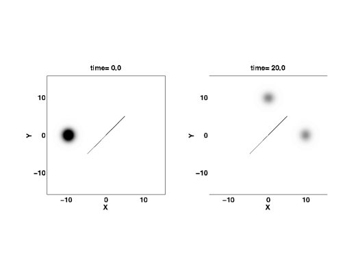
FIG. 4.: The energy density of the photon wave packet which is splitted by a quantum beam splitter composed of a set of two level atoms composing a one-dimensional crystal - the quantum beam splitter. The initial photon is Gaussian (39) with parameters $x_{0}=-10.0$, $y_{0}=0.0$, $k_{x0}=15.0$, $k_{y0}=0.0$, $\Delta_{kx}^{2}=0.125$ and $\Delta_{ky}^{2}=0.125$. The transition frequency $\omega=10.4$ of the atoms is detuned from the central frequency of the incoming photon wave packet $\omega_{0}=15.0$. The total number of atoms is equal to 881, while the number of modes is the same as in the simulation presented in Fig. 2. Here we again assume the dipole constant of the atoms to be $D=0.5$.

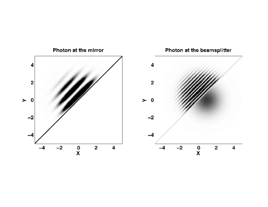
FIG. 5.: The energy density of the electromagnetic field at the moment when the incoming wave packet interfere with the radiation re-emitted by the atoms of the mirror (left) and the beam splitter (right). The central wavelength of the photon wave packet in the case of the mirror simulations is taken to be longer compared to the case of the beam splitter simulations. The interference pattern in the two cases is different. We see that in the case of the beam splitter part of the radiation is transmitted. The parameters of the simulations are specified in previous figures.

In the right hand part of Fig. 5 energy density of the photon wave packet is shown close to the “surface” of the beam splitter. To the left of the atoms the incoming and reflected wave packets interfere. We also see that a fraction of the original radiation is able to “pass” the atoms and to continue to propagate to the right. The wavelength of the photon was chosen shorter than in the mirror simulation, which can be seen from the interference structure.

We have also studied spectral properties of reflected and transmitted parts of the original wave packet. In this situation 200 atoms were used to detect the time dependent spectra of the two outgoing parts of the photon by applying the method described earlier. Both spectra were identical to the spectrum of the incoming photon. This means that our quantum beam splitters and mirrors are linear devices, which is important if we want to build optical networks out of the considered optical elements.

D Parabolic mirror

Another illustration of the power of our microscopic model of optical elements is the parabolic mirror. In fact, it is possible to “build” out of two-level atoms mirrors of arbitrary shapes. In the next simulation, the photon wave packet is propagating towards a parabolic mirror the shape of which is described by the equation $x=x_{0}+\frac{1}{2p}y^{2}=2-\frac{1}{18}y^{2}$. The focus of the parabola is at the point $x=x_{0}+\frac{p}{2}=-2.5$, $y=0$. The time evolution of the energy density is shown in Fig. 6. At $t=0.0$ the Gaussian photon is propagating towards the parabola. The little circle in between the photon and the parabola shows the position of the focus. At $t=8.0$ we see the photon wave packet being reflected from the parabola. We see the interference between the incoming and the re-emitted radiation. We note that at $t=12.8$ most of the radiation goes through the focus. In the last figure ($t=18.0$) the photon wave packet propagates to the left.

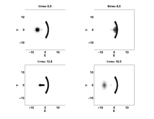
FIG. 6.: The time evolution of the energy density of the one-photon wave packet reflected by a parabolic mirror composed of two-level atoms. At time $t=0$ the wave packet is localized to the left of the focus of the mirror (a little circle in the figure) and propagates towards it. At time $t=8.0$ we see an interference pattern due to interference between the incoming wave packet and the re-emitted radiation. At time $t=12.8$ the original wave packet is completely reflected by the mirror and is localized around the focus. The spatial dependence of the energy density is determined by the shape of the mirror. We can observe a reduction of the width of the reflected wave packet in the $y$ direction. At time $t=18.0$ the wave packet is spread significantly. We see that the maximal energy density is now smaller than in the original wave packet (compare with figure $t=0.0$). The number of atoms from which the parabolic mirror is composed is $N_{A}=1100$. The parameters of the atoms are the same as in Fig. 3. The initial photon is Gaussian (39) with parameters $x_{0}=-6.0$, $y_{0}=0.0$, $k_{x0}=5.0$, $k_{y0}=0.0$, $\Delta_{kx}^{2}=0.125$ and $\Delta_{ky}^{2}=0.125$.

E Interferometer

Using a quantum beam splitter and two quantum mirrors we can “construct” a single-photon interferometer (see Fig. 7). Here the one-photon wave packet comes towards the beam splitter ($t=0.0$) and is divided into two parts which propagate towards the mirrors ($t=18.0$). The distances of the mirrors from the beam splitter are exactly the same. The mirrors reflect the radiation back to the beam splitter. At $t=33.3$ the two reflected parts reach the beam splitter. Each wave packet considered individually would be splitted by the beam splitter into two parts going left and up (i.e. transmitted and reflected).

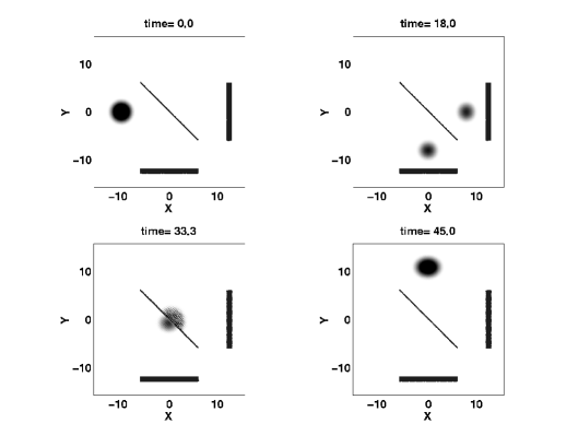
FIG. 7.: The time evolution of the energy density of the one-photon wave packet in an interferometer. The distance of the two mirrors from the beam splitter is the same. We see that the interference results in a wave packet propagating upwards. The initial wave packet, the beam splitter and the mirrors have the same parameters as in figures considered above. Here the mirrors and the beam splitter are specified in Figs. 3 and 4, respectively.

On the other hand due to the quantum interference between the components of the radiation field coming from the two mirrors we can observe something completely different: If the optical paths of the two components are equal then their relative relative phase is such that quantum interference results in an emergence of a single-photon wave packet traveling up ($t=45.0$). On the contrary, if the distances of the two mirrors from the beam splitter are not equal then the relative phase of the two components which interfere on the beam splitter after being reflected by the mirrors can result in a wave packet traveling left (see Fig. 8). Here the difference of the optical paths is approximately one central wavelength of the original wave packet. We see that in this case most of the energy travels in a form of a wave packet to the left.

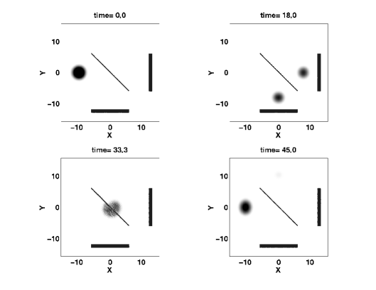
FIG. 8.: Same as in Fig. 7 except the distances of the mirrors from the beam splitter differ by one wavelength. This difference leads to a quantum interference which results in a wave packet propagating to the left. The initial wave packet, the beam splitter and the mirrors have the same parameters as in figures considered above.

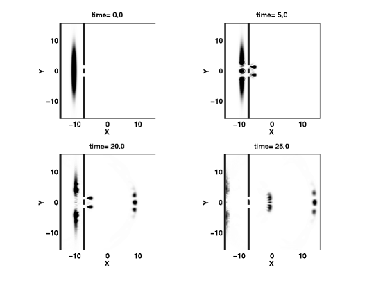
FIG. 9.: The time evolution of the energy density of a photon wave packet in the two-slit experiment. A “plane” wave packet propagates towards the mirror with two slits. The mirror is composed of two level atoms as in previous figures except in this case there are two slits now. Another quantum mirror is considered to be located to the left of the two-slit mirror. This configuration is chosen to make sure that none of the original energy passes to the right due to the periodic conditions we imposed on the Schrödinger equation. To make the figure more transparent we use a logarithmic scale for the energy density of the field. The number of modes in this simulation is $512\times 512$. The total number of atoms used in the mirrors is $N_{A}=7872$.

F Two-slit experiment

The microscopic quantum model we study in this paper can be also used to study the two-slit experiment. Let us assume the photon wave packet which has a very broad energy density in the $y$-direction, i.e. this wave packet models a plane wave which approaches the mirror with two slits, see Fig. 9. On the left we have placed another mirror. Without it, the part of the plane wave which is reflected from the double slit mirror would disappear at the left and reappear on the right because of the periodic boundary conditions we use in our simulations.

The original one-photon wave packet ($t=0.0$) propagates towards the mirror with two slits. At $t=5.0$ the “plane” wave packet is reflected from mirror. Some of the energy propagates through the slits (i.e. there is a nonzero probability that the original one-photon wave packet can be transmitted through the mirror via the slits). We see that through each slit a part of the energy propagates to the right - the interference between these components of the electromagnetic field are clearly seen (see $t=20.0$ and $t=25.0$).

The “plane” wave packet which has been reflected by the mirror with two slits is then reflected by the left mirror and then again by the the double slit mirror. Here part of the energy “goes” through the slits again forming a second, more complex, interference pattern (see $t=20.0$). This process of bouncing of the original wave packet between two mirror continues and each time a fraction of the energy passes through the slits.

It is interesting to compare the interference structure with the theoretical prediction derived within classical optics. The formula can be calculated using Huygens’ principle [18]. According to this, every point at the slit can be considered to be a source of secondary wavelets. The total intensity profile is a superposition of these wavelets. Let us first consider a text book treatment of a one slit mirror, Fig. 10.

FIG. 10.: We show one slit in the mirror. The width of the slit is $d$. The optical path difference of the radiation coming from two different points at the slit is $\Delta x$.

The plane wave packet of the frequency $\omega$ is coming from the left towards a slit of a width $d$. The field strength on the right coming from a specific point at the slit is proportional to the phase factor $e^{i(kx-\omega t)}$. The phase difference of the radiation coming from two different spatial points in the slit is $\Delta x=y\sin\theta$, if the distance from the mirror is long enough. According to the Huygens’ principle the total radiation is a superposition

$$E \propto e^{i(kx-\omega t)}\int\limits_{-d/2}^{d/2}e^{iky\sin\theta}dy$$ (73)

$$= e^{i(kx-\omega t)}\frac{2}{k\sin\theta}\sin(\frac{kd}{2}\sin\theta).$$ (74)

For two slits of width $d$ and a separation $a$ we have two integrals

$$E \propto e^{i(kx-\omega t)}\left(\int\limits_{-d/2}^{d/2}e^{iky\sin\theta}dy+\int\limits_{-a-d/2}^{-a+d/2}e^{iky\sin\theta}dy\right)$$ (75)

$$= e^{i(kx-\omega t+\frac{ka}{2})}\frac{\cos(\frac{ka}{2}\sin\theta)\sin(\frac{kd}{2}\sin\theta)}{k\sin\theta},$$ (76)

which gives for the intensity

$$I\propto E^{*}E=\frac{\cos^{2}(\frac{ka}{2}\sin\theta)\sin^{2}(\frac{kd}{2}\sin\theta)}{(k\sin\theta)^{2}}.$$ (77)

On the other hand, we can use results of our numerical simulations and evaluate the intensity of the radiation which has been created to the right of the two-slit mirror during the first reflection of the original wave packet:

$$I(\phi)=\int\limits_{r_{min}}^{L/2}I(r,\phi)dr.$$ (78)

To neglect the contribution of the second reflection we take the lower bound of the integral over the polar coordinate $r$ to be $r_{min}=10$. The theoretical prediction (77) and the intensity derived from our simulations (78) are shown in Fig. 11. Both intensities are normalized in such a way that their maximum is equal to unity. Near $\theta=0$ the agreement between the two results is very good. For larger values of $\theta$ there is a difference between the two lines which is understandable because we are comparing a classical result with a numerical simulation of a quantum model with realistic features such as the nonzero width of a mirror composed of two-level atoms or the wave packet which is not a plane wave, etc. Taking these differences into account it is surprising that the two pictures coincide so well.

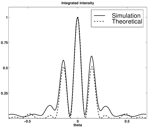
FIG. 11.: We present the intensity of the radiation field at the region behind the two-slit mirror. The dashed line corresponds to the intensity derived from a classical model [see Eq.(78)] while the solid line is obtained from our numerical simulations based on purely quantum description of the process. We see a very good agreement between the two results for small $\theta$.

G Decay of a two level atom

Till now we have considered in our simulations that the field has been initially excited and all the atoms were initially in the ground state. Obviously, our model can be also applied to a situation when one of the atoms is excited and the field is initially in the vacuum state (i.e., we still restrict ourselves to the one-excitation subspace of the total Hilbert space). In this section we briefly discuss the problem of a spontaneous decay of a two-level atom in a two-dimensional cavity. We consider the atomic transition frequency to be $\omega=15.0$ and the dipole constant is $D=0.05$. The atom is situated at the origin ($x=0.0$, $y=0.0$) of the two-dimensional cavity. The number of the field modes is 256$\times$256=65536. In Fig. 12 we present the natural logarithm of the excitation probability of the atom as a function of time. From here we can conclude that the decay of the atom is approximately exponential with a decay constant $\Gamma\simeq 0.14$. In Fig. 13 we present probabilities of the excitation of the modes $k_{x}$ ($k_{y}$=0). Because the direction of the constant dipole vector of the atom is chosen to be in the $z$-direction, the amplitude profile is the same on any line which goes through the origin of the momentum space. As expected for times large enough the modes with $|k_{x}|=15$ are dominantly excited. In fact the peaks are not exactly at the resonance frequency, there is a small shift which is identified to be a Lamb shift (from the figures we cannot see this but the shift can be determined from numerical values obtained in the simulation).

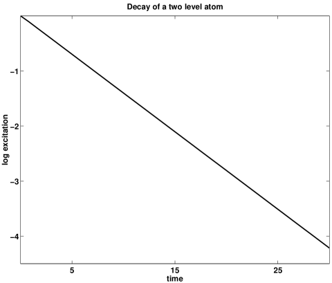
FIG. 12.: The exponential decay of an excited atom. The atomic transition frequency and dipole constants are $\omega=15.0$ and $D=0.05$, respectively. The atom is positioned in the center of the square cavity of the linear dimension $L=10\pi$. We consider $256\times 256=65536$ modes of the electromagnetic field. The probability to find the atom in the excited state is plotted in the logarithmic scale - the exponential character of the decay is clearly seen. The corresponding decay rate is $\Gamma=0.14$.

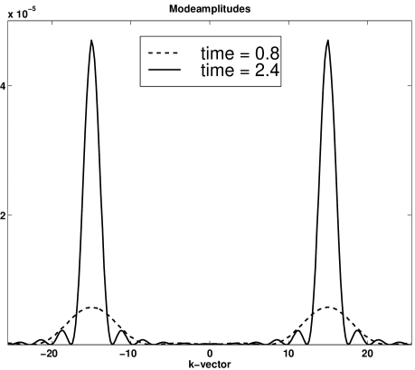
FIG. 13.: We present probabilities of the excitation of the modes with $k_{y}=0$. We see that for times large enough the modes with $|k_{x}|=15$ are dominantly excited, i.e. the field mode at frequencies close to the resonant transition frequency of the atom are most excited.

We plot the energy density of the one-photon wave packet emitted by the decaying atom in Fig. 14. Because of the rotational symmetry of the problem we plot just one “cut” ($y=0$) in the energy density as a function of $x$. The energy density is presented for two times $t=4.0$ and $t=12.0$. At both times there is a peak in the center where the atom is positioned. This means that at these two times the atom still emits the radiation (which is in agreement with the chosen decay rate $\Gamma=0.14$). We turn our attention to the fact that at $t=4.0$ the energy density is nonzero only for $|x|\leq 4.0$. Analogously for the time $t=12.0$ the energy density is nonzero only for $|x|\leq 12.0$. This reflects the fact that the causality is preserved in our simple quantum-mechanical treatment of the decay of the two-level atom in the cavity. Here we have presented just few features of the decay, the complete description of the process deserves more detailed discussion. For instance, one might be interested on how the decay depends on the mode spectra, the position of the atom, what are the values of the Lamb shift, how the decay depends on the frequency cut-off, etc. We will address these questions elsewhere.

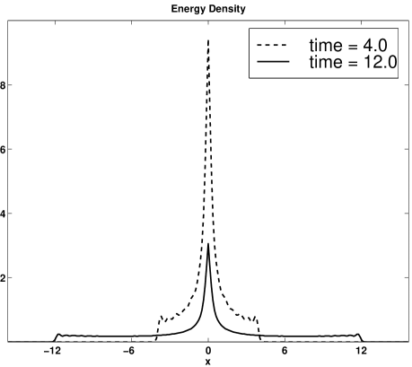
FIG. 14.: We plot the energy density of the one-photon wave packet emitted by the decaying atom. The parameters of the atom are the same as in Fig. 12

V Conclusion

We have shown the results of many quantum mechanical simulations with two level atoms and a one photon wave packet inside a two dimensional cavity. The initial basis vectors are restricted to admit only one excitation. Because a rotating wave interaction between the radiation and the atoms is used, basis vectors with more excitations acquire no excitation. For these kinds of states the special numerical technique which utilizes FFT (Fast Fourier Transform) may be used. Using FFT the simulations become orders of magnitude faster, allowing more modes and atoms to be included.

The atoms are at fixed positions and it is possible to build complicated structures with different kinds of atoms. Several layers of atoms which are on resonance with the incoming radiation form a quantum mechanical mirror if the density of the atoms is high enough. The mirror may have an arbitrary shape. In our simulations usual flat and parabolic mirror were used. One layer of detuned atoms forms a beam splitter. We have shown that, using mirrors and beam splitters, it is possible to build complicated optical networks. As an example the time evolution of a photon in an interferometer was studied.

Usually the optical components are taken to be classical objects which give boundary conditions to the quantum mechanical time evolution or determine the modes used in a quantization. In our simulations the whole system including beam splitters and mirrors is in a well-defined quantum mechanical state. In addition to the simulations shown in this paper is is possible to build more complicated networks of beam splitters and mirrors. One interesting possibility is to build cavities of arbitrary shape and study the time evolution of the photon intensity inside the cavity. It is also possible to use moving atoms in the simulations allowing moving beam splitters and mirrors to be built. One extension of the current model would be to take basis states with more than one photon excitation into account. However, the number of basis states with a given excitation increases so rapidly that it is unlikely to be possible to use the methods of this paper for fields of higher intensity. Thus all the phenomena of nonlinear optics require novel computational approaches.

VI Acknowledgements

We want to thank the Academy of Finland and the Slovak Academy of Sciences for the financial support. This work was supported in part by the Royal Society. Computers of the Center for Scientific Computing (CSC) were used in the simulations. In many computer programs the C++ class library “blitz” developed by Todd Veldhuizen was used (http://monet.uwaterloo.ca/blitz/ ). Finally we want to thank K-A. Suominen for reading the preprint and correcting several misprints.

REFERENCES

- [1] Loudon, R., 1983, The Quantum Theory of Light, 2nd ed. (Clarendon Press, Oxford).
- [2] Milburn, G.J., and Walls, D.F, 1994, Quantum Optics, (Springer, Berlin).
- [3] Mandel, L., and Wolf, E., 1995, Optical Coherence and Quantum Optics, (Cambridge University Press, Cambridge).
- [4] Gardiner. C.W., 1991, Quantum Noise, (Springer, Berlin).
- [5] Steane, A., 1998, Rep. Prog. Phys. 61, 117.
- [6] Advances in Atomic, Molecular and Optical Physics, Supp. 2, “Cavity QED”, 1994, edited by P.R. Berman (Academic Press, New York).
- [7] Weissman, Y., Optical Network Theory, 1992, (Artech House, Boston).
- [8] Ekert, A.K., and Knight, P.L., 1990, Phys.Rev. A 42, 487; 1991, ibid, 43, 3934.
- [9] Stenholm, S., 1994, J. mod. Optics 41, 2483.
- [10] Törmä, P., and Stenholm, S., 1995, J. mod. Optics 42, 1109.
- [11] Stenholm, S., 1995, Appl. Phys. B 60, 243.
- [12] Bužek, V., Drobný, G., Kim, M.G., Havukainen, M and Knight, P.L., 1998, Numerical simulations of fundamental processes in cavity QED: Atomic decay, LANL e-print archive quant-ph/9812001.
- [13] Bužek, V., 1989, Czech. J. Phys. B 39, 345; see also Bužek, and Kim, M.G., 1997, J. Korean Phys. Soc. 30, 413.
- [14] Press, W.H., Teukolsky, S.A., Vetterling, W.T., and Flannery, B.P., 1995, Numerical Recipes in C, 2nd ed., (Cambridge University Press, Cambridge), chapter 16.1.
- [15] Havukainen, M., and Stenholm, S., 1998, J. mod. Optics 45, 1699.
- [16] Eberly, J.H., and Wódkiewicz, K., 1977, J. Opt. Soc. Am. 67, 1252.
- [17] Born, M., and Wolf, E., 1980, Principles of Optics, 6th edn. (Pergamon Press, Oxford).
- [18] Möller, K.D., 1988, Optics, (University Science Books, Mill Valley, California).