Non-Markovian quantum feedback from homodyne measurements: the effect of a non-zero feedback delay time

Abstract

We solve exactly the non-Markovian dynamics of a cavity mode in the presence of a feedback loop based on homodyne measurements, in the case of a non-zero feedback delay time. With an appropriate choice of the feedback parameters, this scheme is able to significantly increase the decoherence time of the cavity mode, even for delay times not much smaller than the decoherence time itself.

I Introduction

Although feedback schemes have been used for long times to control noise, a general theory of feedback for quantum systems has been developed only some years ago by Wiseman and Milburn [1, 2, 3]. Interesting possibilities are opened by the ability to control systems at the quantum level using appropriate feedback loops and some of them have been showed in a series of papers [4, 5, 6, 7, 8, 9]. Ref. [4] has shown that an electro-optical feedback loop based on homodyne measurements of a cavity mode provides an affordable way to realize a squeezed bath for the mode. As a consequence, homodyne-mediated feedback can be used to get squeezing [5], and, in the case of optical cavities with an oscillating mirror, it can be used to significantly cool the mirror. This fact can be extremely useful for the interferometric detection of gravitational waves [8]. The application of a feedback loop realizes an effective “reservoir engineering” [10] and therefore it can be useful also for decoherence control, which is a rapidly expanding field since decoherence is the main limiting factor for quantum information processing [11]. Refs. [5, 6, 7, 9] have already shown that the decoherence induced by photon leakage in electromagnetic cavities can be significantly suppressed with appropriate feedback loops, using the homodyne photocurrent in [5, 6] and direct photodetection and atomic injection in [7, 9].

However, all the relevant applications considered up to now always assume the zero feedback delay time limit $\tau\rightarrow 0$, which is much easier to handle because the problem becomes Markovian and the effect of feedback can be expressed in terms of an effective master equation [1, 2, 3]. The presence of a non-zero delay has been considered briefly only in [3], where the spectrum of a homodyne measurement has been evaluated for a simple case. The Markovian treatment is justified whenever the feedback delay time is much smaller than the typical cavity timescale. If one considers squeezing or some other stationary state phenomenon, the feedback delay time $\tau$ has to be compared with the cavity relaxation time $\gamma^{-1}$ and for sufficiently good cavities the Markovian condition $\gamma\tau\ll 1$ is usually satisfied. However, if one considers the feedback scheme for decoherence control, the delay $\tau$ has to be negligible with respect to the decoherence time $t_{dec}\simeq(\gamma\bar{n})^{-1}$, which can be much shorter than the damping time when the cavity mean photon number $\bar{n}$ is large. In these cases, the unavoidable non-zero feedback delay time may have important effects and it would be important to deal with the exact non-Markovian problem with $\tau\neq 0$. There is in fact a renewed interest in non-Markovian effects, which can play an important role when considering quantum optics in high-Q cavities and in photonic bandgap materials. For this reason, non-Markovian trajectory theories have been recently developed in Refs. [12, 13, 14].

The quantum theory of feedback has been developed by Wiseman and Milburn in [1, 2] using quantum trajectory theory [15], and only later Wiseman showed an equivalent derivation based on the input-output theory [16, 17, 18] in Ref. [3]. However Ref. [3] proved the equivalence between the two approaches in the perfect detection $\eta=1$ case only. In this paper we shall see how to extend the quantum Langevin approach of the input-output theory to the non-unit efficiency case and we shall see that this theoretical framework is best suited to deal with the non-Markovian case of non-zero feedback delay time. We shall consider the non-Markovian effects by completely solving the dynamics of a cavity mode in the presence of a homodyne-mediated electro-optical feedback loop, which has been already considered (in the zero delay limit only) in Ref. [6].

The paper is organized as follows. In Section II we shall reconsider the quantum theory of feedback in the case of homodyne measurements, adopting the input-output theory of Gardiner and Collett [16, 17, 18] and we shall see how to introduce the non-unit detection efficiency in this framework. In Section III we shall completely solve the non-Markovian dynamics in the presence of a non-zero feedback delay by considering the time evolution of the probability distribution of the measured field quadrature and of the characteristic function. We shall consider in particular the possibility of inhibiting the decoherence of a Schrödinger cat state initially generated in the cavity and we shall see that the significant decoherence suppression which can be obtained, for appropriately chosen feedback parameters, in the zero delay case (see Ref. [6]) is recovered even in the presence of not negligible feedback delay times.

II Homodyne-mediated quantum feedback theory within the input-output formalism

We shall consider an optical cavity, with annihilation operator $a$, subject to the homodyne measurement of the field quadrature

$$X_{\varphi}=\frac{1}{2}(\>a\,e^{-i\varphi}\,+\,a^{\dagger}\,e^{i\varphi}\>).$$ (1)

We shall consider the possibility of applying a feedback loop to this cavity mode, by feeding back part of the output homodyne photocurrent to control in some way the $a$ mode dynamics.

First of all it is convenient to reformulate Wiseman and Milburn quantum theory of feedback [1, 2] using the input-output theory developed by Gardiner and Collett [16, 17]. The input-output formalism is essentially an Heisenberg approach for the whole system (cavity and vacuum bath), in which the environment dynamics is described by the white-noise input operator $dB(t)$ satisfing the Ito rules [16, 17, 18, 19]:

$$\begin{array}[]{c}dB(t)^{2}=dB^{\dagger}(t)^{2}=0,\;\;dB^{\dagger}(t)dB(t)=0,\\ \\ dB(t)dB^{\dagger}(t)=dt,\end{array}$$ (2)

and the following commutation’ s relations:

$$\begin{array}[]{c}\big{[}\,dB(t),dB(t^{\prime})\,\big{]}=0,\\ \\ \big{[}\,dB(t),dB^{\dagger}(t^{\prime})\,\big{]}=\delta(t-t^{\prime})dtdt^{\prime}.\end{array}$$ (3)

In the absence of any feedback loop, the evolution of a generic cavity mode operator $\hat{O}(t)$ in the interaction picture is described by the quantum Langevin equation [16, 17]:

$$d\hat{O}(t) = \frac{\gamma}{2}\big{(}\>2a^{\dagger}(t)\hat{O}(t)a(t)-a^{\dagger}(t)a(t)\hat{O}(t)-\hat{O}(t)a^{\dagger}(t)a(t)\>\big{)}\,dt$$ (5)

$$-\>\sqrt{\gamma}\,\big{[}\hat{O}(t),a^{\dagger}(t)\big{]}\,dB(t)\>+\>\sqrt{\gamma}\,\big{[}\hat{O}(t),a(t)\big{]}\,dB^{\dagger}(t),$$

where $\gamma$ is the cavity damping rate.

Eq. (5) can be solved explicitely in terms of the evolution operator $U(t,t_{0})$

$$\hat{O}(t)=U^{\dagger}(t,0)\hat{O}\,U(t,0),$$ (6)

which in the absence of feedback takes the following form [18]

$$U(t,t_{0})=\,\stackrel{{\scriptstyle\longleftarrow}}{{\exp}}\Big{(}\,\sqrt{\gamma}\int_{t_{0}}^{t}dB^{\dagger}(t^{\prime})a\;-\;\sqrt{\gamma}\int_{t_{0}}^{t}dB(t^{\prime})a^{\dagger}\Big{)},$$ (7)

where $a$ and $a^{\dagger}$ are in the Schrödinger representation and $\stackrel{{\scriptstyle\longleftarrow}}{{\exp}}$ denotes the time-ordered exponential. The evolution operator $U(t,t_{0})$ describes also the evolution in the Schrödinger representation, [18, 19],

$$|\Psi(t)\rangle_{T}=U(t,0)\;\Big{\{}|\psi_{A}\rangle\otimes|0\rangle\Big{\}},$$ (8)

where the vector $|\Psi(t)\rangle_{T}$ obeys the following stochastic equation

$$d|\Psi(t)\rangle_{T}=\Big{\{}\sqrt{\gamma}\,a\;dB^{\dagger}(t)-\sqrt{\gamma}\,a^{\dagger}\;dB(t)-\frac{\gamma}{2}\,a^{\dagger}a\,dt\Big{\}}|\Psi(t)\rangle_{T}.$$ (9)

Using the commutation’ s rules (3), it is easy to prove that the Heisenberg evolution (6) satisfies the usual requirement that the input noise $dB(t)$ has to commute with every cavity operator evaluated at preceding times $t^{\prime}<t$

$$\big{[}\,dB(t),\hat{O}(t^{\prime})\,\big{]}=\big{[}\,dB^{\dagger}(t),\hat{O}(t^{\prime})\,\big{]}=0\hskip 21.68121pt\mbox{for}\hskip 14.45377ptt\geq t^{\prime}.$$ (10)

Equation (5) can be used to get the time evolution of a generic matrix element of $\hat{O}(t)$ between two state vectors of the whole system of the form $|\psi_{A}\rangle\otimes|0\rangle$ and $|\psi_{B}\rangle\otimes|0\rangle$, in which the environment is left in the vacuum state,

$$d\langle\hat{O}(t)\rangle_{\mbox{{AB}}}=\frac{\gamma}{2}\left\{\,2\langle a^{\dagger}(t)\hat{O}(t)a(t)\rangle_{\mbox{{AB}}}-\langle a^{\dagger}(t)a(t)\hat{O}(t)\rangle_{\mbox{{AB}}}-\langle\hat{O}(t)a^{\dagger}(t)a(t)\rangle_{\mbox{{AB}}}\,\right\}\,dt,$$ (11)

where

$$\langle\hat{O}(t)\rangle_{\mbox{{AB}}}\equiv\Big{\{}\langle 0|\otimes\langle\psi_{A}|\Big{\}}\,\hat{O}(t)\,\Big{\{}|\psi_{B}\rangle\otimes|0\rangle\Big{\}}.$$ (12)

Let us now introduce the feedback loop associated to the homodyne measurement of the quadrature $X_{\varphi}$. Differently from Ref. [3], we assume the possibility of a non-unit homodyne detection efficiency $\eta\leq 1$. The application of a feedback loop is equivalent to add a feedback Hamiltonian $H_{fb}(t)$ [1, 2, 5], so that the correction to the Heisenberg evolution of Eq. (5) takes the form

$$d\hat{O}_{{\em fb}}(t)=\frac{i\sqrt{\gamma}\,dY_{\varphi}(t-\tau)}{\eta}\,\big{[}F(t),\hat{O}(t)\big{]}$$ (13)

where $F(t)$ is the observable of the cavity mode through which the feedback acts on the system and $Y_{\varphi}(t)$ is the output field operator associated to the homodyne measurement. In the quantum trajectory approach of [1, 2], the fed-back homodyne photocurrent $Y_{\varphi}(t)$ is a classical quantity, but in the quantum Langevin approach it must be an operator with its quantum fluctuations. However, one can adopt the general theory of homodyne measurements of Ref. [20] and write the photocurrent operator in an analogous way

$$dY_{\varphi}(t)=2\,\sqrt{\gamma}\eta\,X_{\varphi}(t)\,dt\>+\sqrt{\eta}\>d\,\Xi_{\varphi}(t).$$ (14)

where $d\,\Xi_{\varphi}(t)$ describes the “noisy” part of the output photocurrent operator. The only delicate point in the derivation of the quantum theory of feedback of [1, 2] in the imperfect detection case using the input-output theory is just the exact determination of this noisy operator $d\,\Xi_{\varphi}(t)$. Since $Y_{\varphi}(t)$ is an output operator, it is quite natural to consider Eq. (14) as an input-output relation [16, 17, 19], so that the noisy term would simply be the input field $d\,\Xi_{\varphi}(t)=dB(t)\,e^{-i\varphi}+dB^{\dagger}(t)\,e^{i\varphi}$. However this interpretation of Eq. (14) is correct only in the perfect detection case $\eta=1$, because only in this case the output of the detection apparatus coincides with the cavity output and the quantum fluctuations of the vacuum bath are transferred unaltered by the detector. In the presence of imperfect detection, the output photocurrent may be non trivially related with the input noise $dB(t)$ and in general one has to describe the noisy operator $d\,\Xi_{\varphi}(t)$ in terms of a new noise $dB_{f}(t)$, which we shall call “feedback”noise. Therefore one has to write

$$d\,\Xi_{\varphi}(t)=dB_{f}(t)\,e^{-i\varphi}+dB_{f}^{\dagger}(t)\,e^{i\varphi},$$ (15)

where the feedback noise $dB_{f}(t)$ satisfies the same properties (2) and (3) of the input noise; moreover this feedback noise is correlated with the input noise $dB(t)$ and this correlation is determined just by the detection efficiency $\eta$, since one has

$$\begin{array}[]{c}\big{[}\,dB(t),dB_{f}(t^{\prime})\,\big{]}=0,\\ \\ \big{[}\,dB(t),dB_{f}^{\dagger}(t^{\prime})\,\big{]}=\sqrt{\eta}\delta(t-t^{\prime})dtdt^{\prime}.\end{array}$$ (16)

It is immediate to see that in the perfect detection case $\eta=1$, one can identify the feedback noise with the input noise $dB_{f}(t)=dB(t)$, while in the opposite case $\eta=0$ the two noises are uncorrelated, as it can be easily expected since in this case the fed-back noise has nothing to do with the vacuum input noise.

In the feedback correction (13) of the Heisenberg evolution, $\tau$ is the delay time associated to the feedback loop and since it is a non-negative quantity, it ensures that the output operator $Y_{\varphi}(t-\tau)$ commutes with all system operators evaluated at time $t$. In particular $Y_{\varphi}(t-\tau)$ commutes with $F(t)$ and so there is no ambiguity in the definition of $d\hat{O}_{{\em fb}}(t)$. As it has been stressed in Ref. [1, 2, 5], one must be careful in using (13); the feedback process is physically added to the evolution of the system of interest, so its stochastic differential contribution has to be introduced as limit of a real process. This implies that (13) has to be considered in the Stratonovich sense. Therefore it is convenient to rewrite it in the Ito form and then add it to Eq. (5), so that the resulting equation for $\hat{O}(t)$ becomes

$$\begin{array}[]{c}d\hat{O}(t)=\frac{\gamma}{2}\big{(}\>2a^{\dagger}(t)\hat{O}(t)a(t)-a^{\dagger}(t)a(t)\hat{O}(t)-\hat{O}(t)a^{\dagger}(t)a(t)\>\big{)}\,dt\\ \\ -\>\sqrt{\gamma}\,\big{[}\hat{O}(t),a^{\dagger}(t)\big{]}\,dB(t)\>+\>\sqrt{\gamma}\,\big{[}\hat{O}(t),a(t)\big{]}\,dB^{\dagger}(t)\\ \\ +i\,\sqrt{\gamma}\>\big{(}\>\sqrt{\gamma}a^{\dagger}(t-\tau)\,e^{i\varphi}\,dt+\frac{dB_{f}^{\dagger}(t-\tau)}{\sqrt{\eta}}e^{i\varphi}\>\big{)}\;\big{[}F(t),\hat{O}(t)\big{]}\,\Theta(t-\tau)\\ \\ +i\,\sqrt{\gamma}\;\big{[}F(t),\hat{O}(t)\big{]}\;\big{(}\>\sqrt{\gamma}a(t-\tau)\,e^{-i\varphi}\,dt+\frac{dB_{f}(t-\tau)}{\sqrt{\eta}}e^{-i\varphi}\>\big{)}\,\Theta(t-\tau)\\ \\ -\frac{\gamma}{2\eta}\,\Theta(t-\tau)\big{[}F(t),\big{[}F(t),\hat{O}(t)\big{]}\big{]}dt.\end{array}$$ (17)

This is the quantum Ito stochastic equation describing the time evolution in the presence of feedback and non-unit detection efficiency and it coincides with the quantum Ito equation derived in Ref. [3] in the case of perfect homodyne detection $\eta=1$. We have also explicitely inserted the step function $\Theta(t-\tau)$ with respect to Ref. [3] to stress the impossibility for the feedback to act on the system before the delay time $\tau$ has elapsed since the initial condition. This means that the evolution of $\hat{O}(t)$ for $0\leq t\leq\tau$ coincides with that in absence of feedback, described by Eq. (5). Moreover we observe that, since the equation for $d\,\hat{O}(t)$ contains only stochastic terms evaluated for times $t^{\prime}\leq t$ (precisely $t$ and $t-\tau$), it is possible to conclude that the commutation relations (10) are valid also in the presence of feedback and, more in general, that Eq. (17) preserves the canonical commutation rules for $a(t)$ and $a^{\dagger}(t)$.

A Zero delay time limit

Up to now, the explicit applications of the quantum theory of feedback of Wiseman and Milburn have considered the zero delay time case $\tau=0$ only, when one has a tractable Markovian equation. Whenever one considers a non-zero delay the problem becomes non-Markovian and difficult to solve.

The feedback master equation for homodyne-mediated feedback in the zero delay limit has been first derived in its general form using quantum trajectory theory [15] in Ref. [1, 2]. In the case of perfect homodyne detection $\eta=1$, the same homodyne-mediated feedback equation has been rederived using input-output theory by Wiseman in [3] and, in its linear stochastic form, by Goetsch et al. in Ref. [6]. However, the connection between this linear stochastic approach and the input-output theory was not made explicit there. In reviewing the zero delay time case we shall clarify here the connections between the different approaches and we show in particular that the linear stochastic Schrödinger equation approach of Ref. [6] is equivalent to the input-output result of Eq. (17) (in the case $\eta=1$) in the same way as Eq. (9) is equivalent to the quantum Langevin equation Eq. (5).

The starting point of the analysis of Ref. [6] is the evolution equation for the state vector $|\Psi(t)\rangle_{T}$ of the whole system (cavity and vacuum bath). In the no feedback case, this equation is obviously equal to Eq. (9); the feedback loop is then introduced using the same Hamiltonian modification of (13) in the case $\eta=1$. However, since in Ref. [6] the zero delay time limit is considered from the beginning, one has to be careful with operator ordering, because in this circumstance one is not guaranteed that $dY_{\varphi}(t)$ commutes with the cavity mode operator $F(t)$ at the same time. In Ref. [6] the question is solved by imposing that “the feedback acts later”, i.e., that $|\Psi(t+dt)\rangle_{T}$ is obtained from $|\Psi(t)\rangle_{T}$ by means of $U(t+dt,t)$ (the evolution operator in the absence of feedback loop) first and by the Hamiltonian feedback correction later (see Eq. (2.11) of [6]). It is clear that in this way the equivalence with the input-output approach of Ref. [3] it is not so evident. However the equivalence can be proved by considering the following evolution operator

$$\begin{array}[]{r}U_{F}(t,t_{0})=\,\stackrel{{\scriptstyle\longleftarrow}}{{\exp}}\Big{\{}\int_{t_{0}}^{t}\Big{(}\sqrt{\gamma}dB^{\dagger}(t^{\prime})a\;-\;\sqrt{\gamma}dB(t^{\prime})a^{\dagger}-i\sqrt{\gamma}Fe^{-i\varphi}dB(t^{\prime})\\ \ -i\sqrt{\gamma}Fe^{i\varphi}dB^{\dagger}(t^{\prime})-i\frac{\gamma}{2}a^{\dagger}Fe^{i\varphi}dt^{\prime}-i\frac{\gamma}{2}Fae^{-i\varphi}dt^{\prime}\Big{)}\Big{\}};\end{array}$$ (18)

where $a$, $a^{\dagger}$ and $F$ are in Schrödinger representation. Using the Ito rules (2) to evaluate the differential $d\hat{O}(t)$, it is possible to check that $U_{F}(t,t_{0})$ is just the evolution operator determining the formal solution of Eq. (17) in the $\tau=0$ and $\eta=1$ limit, according to the usual rule

$$\hat{O}(t)=U_{F}^{\dagger}(t,0)\,\hat{O}\,U_{F}(t,0)\;.$$ (19)

As it can be easily expected, the zero delay evolution operator $U_{F}(t,t_{0})$ reduces to the no-feedback one $U(t,t_{0})$ of Eq. (7) when $F=0$. This suggests that an equivalent Schrödinger representation could be obtained also in the case of feedback with zero delay time, starting from an equation analogous to Eq. (8). In fact if we apply $U_{F}(t,0)$ to the initial state of the total system and we use again the Ito rules (2), one gets the following linear stochastic Schrödinger equation,

$$d|\Psi(t)\rangle_{T} = \Big{\{}\sqrt{\gamma}\,a\;dB^{\dagger}(t)-\sqrt{\gamma}\,a^{\dagger}\;dB(t)-\frac{\gamma}{2}\,a^{\dagger}a\,dt$$ (22)

$$-i\sqrt{\gamma}\,F\;d\,\Xi_{\varphi}(t)-i\gamma F\,ae^{-i\varphi}dt-\frac{\gamma}{2}\,F^{2}\,dt\Big{\}}|\Psi(t)\rangle_{T}$$

coinciding with the equation obtained in [6]. This shows that the approach of Ref. [6] and that of Ref. [3] are respectively the Schrödinger and Heisenberg view of the same theory, with $U_{F}(t,t_{0})$ the unitary operator mediating the transition from one to the other.

In Ref. [6], by adopting an appropriate representation basis for the vacuum modes (see for example [19]), Eq. (22) was then reduced to a linear stochastic equation for the cavity mode only which was solved numerically. In Appendix A we shall reconsider this linear stochastic equation for the cavity mode and we shall see how it is possible to solve it analytically by adopting the integration method described in [21].

Determining an evolution operator analogous to $U_{F}(t,t_{0})$ for the $\tau\neq 0$ case is much more difficult and we shall not consider this strategy to study the non-zero delay problem. Instead we shall adopt the input-output formalism which has yielded Eq. (17). To be more specific, we shall always consider generic matrix elements as those of Eq. (12), whose evolution equation can be easily derived from Eq. (17):

$$\begin{array}[]{c}\frac{d}{dt}\langle\hat{O}(t)\rangle_{\mbox{{AB}}}=\frac{\gamma}{2}\left\{\>2\langle a^{\dagger}(t)\hat{O}(t)a(t)\rangle_{\mbox{{AB}}}-\langle a^{\dagger}(t)a(t)\hat{O}(t)\rangle_{\mbox{{AB}}}-\langle\hat{O}(t)a^{\dagger}(t)a(t)\rangle_{\mbox{{AB}}}\>\right\}\\ \\ +i\,\gamma\left\{\langle a^{\dagger}(t-\tau)\big{[}F(t),\hat{O}(t)\big{]}\rangle_{\mbox{{AB}}}\,e^{i\varphi}\,+\,\langle\big{[}F(t),\hat{O}(t)\big{]}a(t-\tau)\rangle_{\mbox{{AB}}}\,e^{-i\varphi}\right\}\Theta(t-\tau)\\ \\ -\frac{\gamma}{2\eta}\,\langle\big{[}F(t),\big{[}F(t),\hat{O}(t)\big{]}\big{]}\rangle_{\mbox{{AB}}}\;.\Theta(t-\tau).\end{array}$$ (23)

III Feedback dynamics in the presence of a non-zero delay

The dynamics in the presence of a feedback loop with a non-zero delay time has never been completely solved because of its intrinsic non-Markovian nature. In this paper we shall analyze the effects of a non-zero feedback delay by considering a specific example for the “feedback operator” $F(t)$

$$F(t)=g\,X_{\theta}(t)=\frac{g}{2}(\>a(t)\,e^{-i\theta}\,+\,a^{\dagger}(t)\,e^{i\theta}\>),$$ (24)

where the constant $g$ represents the gain of the feedback process and $\theta$ is an experimentally controllable phase. The particular choice (24) of $F$ means that the feedback loop adds a driving term to the mode dynamics, which could be achieved, e. g. , by using an electro-optic device with variable transmittivity driven by the homodyne photocurrent. The homodyne-mediated feedback model with the choice (24) for $F(t)$ has been completely solved in Ref. [6] in the Markovian limit of zero delay time and therefore the comparison with the results of Ref. [6] will be very instructive. As it is shown in Ref. [6], the main virtue of the homodyne-mediated feedback is its capability of slowing down the decoherence associated with cavity damping provided that the feedback parameters $g$ and $\theta$ are appropriately chosen. Here we shall see that the decoherence inhibition caused by the feedback takes place also in the presence of a non-zero feedback delay time; in particular, decoherence is appreciably slowed down even for delay times not much smaller than the decoherence time itself.

First of all we shall show the exact time evolution for the marginal probability distribution $P(x_{\varphi},t)$ of the quadrature component $X_{\varphi}(t)$: this will result in a quite simple expression which can be easily analysed. Then we shall give the complete solution of the system dynamics in terms of the symmetrically ordered characteristic function.

A The marginal probability distribution

A good, even if not complete, description of the state of the cavity mode is given by the marginal probability distribution $P(x_{\varphi},t)$ of the measured quadrature component $X_{\varphi}(t)$. We shall consider the following class of initial states for the whole system

$$\rho_{T}(0)=\sum_{\mbox{{$\alpha,\beta$}}}N_{\mbox{{$\alpha,\beta$}}}|\alpha\rangle\langle\beta|\otimes|0\rangle\langle 0|,$$ (25)

i.e. a linear superposition of coherent states for the cavity mode and the vacuum state for the electromagnetic bath. We shall focus on the evaluation of the moments

$$\langle X_{\varphi}^{N}(t)\rangle_{\mbox{{$\beta\alpha$}}}\equiv\Big{\{}\langle 0|\otimes\langle\beta|\Big{\}}\,X_{\varphi}^{N}(t)\,\Big{\{}|\alpha\rangle\otimes|0\rangle\Big{\}}$$ (26)

($N$ is an integer). $P(x_{\varphi},0)$ is a superposition of Gaussian functions and, thanks to the choice of Eq. (24) for the feedback operator, the evolution in the presence of feedback remains linear, so that $P(x_{\varphi},t)$ will maintain its initial Gaussian behaviour. This fact will be explicitely verified at the end of the section.

We now proceed step by step: first we explicitely determine the evolution of the first and second order moment and then we derive a recursive relation between the moments clearly showing the Gaussian nature of the corresponding probability distribution.

For $N=1$ Eq. (26) becomes the matrix element of the measured quadrature $X_{\varphi}(t)$, and Eqs. (23) and (24) yield the following differential equation for its evolution

$$\frac{d}{dt}\langle X_{\varphi}(t)\rangle_{\mbox{{AB}}}=-\frac{\gamma}{2}\langle X_{\varphi}(t)\rangle_{\mbox{{AB}}}+\gamma\,g\sin(\theta-\varphi)\langle X_{\varphi}(t-\tau)\rangle_{\mbox{{AB}}}\Theta(t-\tau),$$ (27)

which can be integrated for $t\geq 0$ using Laplace transforms as it is discussed in Appendix B:

$$\langle X_{\varphi}(t)\rangle_{\mbox{{AB}}}=\langle X_{\varphi}(0)\rangle_{\mbox{{AB}}}\chi(t)$$ (28)

with

$$\chi(t)=\sum_{n=0}^{[t/\tau]}\frac{\big{(}g\sin(\theta-\varphi)\big{)}^{n}}{n!}\,e^{-\frac{\gamma}{2}(t-n\tau)}\,\big{(}\gamma\,(t-n\tau)\big{)}^{n},$$ (29)

where $[x]$ indicates the integer part of the real number $x$. In the case of the initial condition (25), one has simply to consider $|\psi_{A}\rangle\equiv|\beta\rangle$ and $|\psi_{B}\rangle=|\alpha\rangle$ in Eq. (28), even though it is clear that this solution is valid for any choice of the initial state of the cavity. The function $\chi(t)$ of Eq. (29) will often appear in the complete analytical solution of the problem described in the following and it is therefore useful to describe its behavior in the various limits. The solution (28) has the correct behavior both in the $g\rightarrow 0$ limit, where one has the simple exponential decay $\chi(t)=e^{-\gamma t/2}$, and in the $\tau\rightarrow 0$ limit, yielding

$$\chi(t)=\exp\Big{\{}-\frac{\gamma}{2}\,\big{(}1-2g\sin(\theta-\varphi)\big{)}\,t\Big{\}},$$ (30)

which is the same solution which can be derived from the exact treatment of Ref. [6]. It is interesting to consider the limit of small delay, $\gamma\tau\ll 1$, because this condition can be easily verified using good optical cavities and common electro-optical feedback loops. From the exact solution (29) one gets

$$\chi(t)=\Big{\{}1-\frac{g\sin(\theta-\varphi)}{2}\,\Big{(}2-\gamma t(1-2g\sin(\theta-\varphi))\Big{)}\gamma\tau\Big{\}}\,e^{-(1-2g\sin(\theta-\varphi))\frac{\gamma}{2}t}.$$ (31)

We have plotted the solution (29) in Fig. 1, in which there is also a comparison with the no feedback case and with the Markovian feedback case of the zero delay time limit. This plot makes evident how the major part of the difference between the zero delay and the delayed cases comes from the retardation caused by the presence of $\Theta(t-\tau)$: for simplicity, we shall refer in the following to this effect as the “step effect”.

For the determination of the second order moment (Eq. (26) with $N=2$) it is convenient to study the correlation function $C(t,t^{\prime})=\langle X_{\varphi}(t)X_{\varphi}(t^{\prime})\rangle_{\mbox{{$\beta\alpha$}}}$ for every positive values of $t$ and $t^{\prime}$. We first focus on the dependence on $t^{\prime}$ and differentiate $C(t,t^{\prime})$ by $t^{\prime}$ using Eq. (17), so to get the following differential equation:

$$d\;C(t,t^{\prime}) = -\frac{\gamma}{2}C(t,t^{\prime})\,dt^{\prime}+\gamma\,g\sin(\theta-\varphi)C(t,t^{\prime}-\tau)\Theta(t^{\prime}-\tau)\,dt^{\prime}$$ (34)

$$-\frac{\sqrt{\gamma}}{2}e^{i\varphi}\langle\big{[}X_{\varphi}(t),dB^{\dagger}(t^{\prime})\big{]}\rangle_{\mbox{{$\beta\alpha$}}}+\sqrt{\frac{\gamma}{4\eta}}g\sin(\theta-\varphi)e^{i\varphi}\langle\big{[}X_{\varphi}(t),dB_{f}^{\dagger}(t^{\prime}-\tau)\big{]}\rangle_{\mbox{{$\beta\alpha$}}}\Theta(t^{\prime}-\tau).$$

The corresponding initial condition can be obtained from Eq. (28) and is given by $C(t,0)=\langle X_{\varphi}(0)X_{\varphi}(0)\rangle_{\mbox{{$\beta\alpha$}}}\,\chi(t)$. Now Eq. (34) can be explicitely integrated once that the explicit $t^{\prime}$ dependence of the commutators between the noises $dB^{\dagger}(t^{\prime})$ and $dB_{f}^{\dagger}(t^{\prime}-\tau)$ and the operator $X_{\varphi}(t)$ is known. For the determination of these commutators, let us define first of all $f(t,t^{\prime})=\big{[}X_{\varphi}(t),B^{\dagger}(t^{\prime})\big{]}$, in which $B^{\dagger}(t^{\prime})$ is the sum of all the Ito increments of the input noise from the initial time up to $t^{\prime}$. Now we can proceed in an analogous way as we have done to write Eq.(34) and we differentiate in $t$ by keeping $t^{\prime}$ constant. Using the commutation rules of Eq. (3) we get

$$\frac{\partial}{\partial t}f(t,t^{\prime}) = -\frac{\gamma}{2}f(t,t^{\prime})+\gamma\,g\sin(\theta-\varphi)f(t-\tau,t^{\prime})\Theta(t-\tau)$$ (37)

$$-\frac{\sqrt{\gamma}}{2}e^{-i\varphi}\Big{\{}\Theta(t^{\prime}-t)-g\sin(\theta-\varphi)\Theta(t-\tau)\Theta(t^{\prime}-t+\tau)\Big{\}}.$$

which, except for the presence of last term which is a known function of time, is an equation similar to Eq. (27) and therefore can be solved using Laplace transforms and the initial condition $f(0,t^{\prime})=0$ implied by Eq. (10). The commutation rules between $X_{\varphi}(t)$ and the Ito increment $dB^{\dagger}(t^{\prime})$ can now be obtained by simply differentiating this solution with respect to $t^{\prime}$ and the final result is

$$\big{[}X_{\varphi}(t),dB^{\dagger}(t^{\prime})\big{]}={\cal F}(t,t^{\prime})\,dt^{\prime}$$ (38)

where

$${\cal F}(t,t^{\prime})=-\frac{\sqrt{\gamma}}{2}e^{-i\varphi}\Big{\{}\Theta(t-t^{\prime})\chi(t-t^{\prime})-g\sin(\theta-\varphi)\,\Theta(t-t^{\prime}-\tau)\;\chi(t-t^{\prime}-\tau)\Big{\}}\equiv{\cal F}(t-t^{\prime}).$$ (39)

The same procedure can be adopted to determine the commutator $\big{[}X_{\varphi}(t),dB_{f}^{\dagger}(t^{\prime})\big{]}$ involving the feedback noise and one finally gets

$$\big{[}X_{\varphi}(t),dB_{f}^{\dagger}(t^{\prime})\big{]}={\cal F}_{f}(t,t^{\prime})\,dt^{\prime}$$ (40)

where

$${\cal F}_{f}(t,t^{\prime})=-\frac{\sqrt{\gamma}}{2}e^{-i\varphi}\Big{\{}\sqrt{\eta}\Theta(t-t^{\prime})\chi(t-t^{\prime})-\frac{g\sin(\theta-\varphi)}{\sqrt{\eta}}\,\Theta(t-t^{\prime}-\tau)\;\chi(t-t^{\prime}-\tau)\Big{\}}\equiv{\cal F}_{f}(t-t^{\prime}).$$ (41)

Proceeding as before it is possible to compute also the commutation rules between the noise operators $dB(t^{\prime})$, $dB^{\dagger}(t^{\prime})$, $dB_{f}(t^{\prime})$, $dB_{f}^{\dagger}(t^{\prime})$ and $a(t)$, $a^{\dagger}(t^{\prime})$ which we explicitely report here because they will be useful in the following

$$\begin{array}[]{ll}\big{[}a(t),dB(t^{\prime})\big{]}={\cal R}(t,t^{\prime})\,dt^{\prime}&\big{[}a(t),dB^{\dagger}(t^{\prime})\big{]}=-{\cal R}_{1}^{*}(t,t^{\prime})\,dt^{\prime}\\ \\ \big{[}a^{\dagger}(t),dB(t^{\prime})\big{]}={\cal R}_{1}(t,t^{\prime})\,dt^{\prime}&\big{[}a^{\dagger}(t),dB^{\dagger}(t^{\prime})\big{]}=-{\cal R}^{*}(t,t^{\prime})\,dt^{\prime},\\ \\ \big{[}a(t),dB_{f}(t^{\prime})\big{]}={\cal R}^{f}(t,t^{\prime})\,dt^{\prime}&\big{[}a(t),dB_{f}^{\dagger}(t^{\prime})\big{]}=-{\cal R}_{1}^{f\,*}(t,t^{\prime})\,dt^{\prime}\\ \\ \big{[}a^{\dagger}(t),dB_{f}(t^{\prime})\big{]}={\cal R}_{1}^{f}(t,t^{\prime})\,dt^{\prime}&\big{[}a^{\dagger}(t),dB_{f}^{\dagger}(t^{\prime})\big{]}=-{\cal R}^{f\,*}(t,t^{\prime})\,dt^{\prime},\end{array}$$ (42)

where

$${\cal R}(t,t^{\prime}) = i\frac{\sqrt{\gamma}}{2}\,g\,e^{i(\theta+\varphi)}\Big{\{}\Theta(t-t^{\prime}-\tau)\Big{[}e^{-\frac{\gamma}{2}(t-t^{\prime}-\tau)}-\frac{\chi(t-t^{\prime})-e^{-\frac{\gamma}{2}(t-t^{\prime})}}{g\sin(\theta-\varphi)}\Big{]}$$ (45)

$$+\Theta(t-t^{\prime}-2\tau)\big{[}\chi(t-t^{\prime}-\tau)-e^{-\frac{\gamma}{2}(t-t^{\prime}-\tau)}\big{]}\Big{\}}\equiv{\cal R}(t-t^{\prime}),$$

$${\cal R}_{1}(t,t^{\prime})=-2e^{-i\varphi}{\cal F}^{*}(t,t^{\prime})-e^{-2i\varphi}{\cal R}(t,t^{\prime})\equiv{\cal R}_{1}(t-t^{\prime}).$$ (46)

$${\cal R}^{f}(t,t^{\prime}) = i\sqrt{\frac{\gamma}{4\eta}}\,g\,e^{i(\theta+\varphi)}\Big{\{}\Theta(t-t^{\prime}-\tau)\Big{[}e^{-\frac{\gamma}{2}(t-t^{\prime}-\tau)}-\frac{\eta\left(\chi(t-t^{\prime})-e^{-\gamma(t-t^{\prime})/2}\right)}{g\sin(\theta-\varphi)}\Big{]}$$ (49)

$$+\Theta(t-t^{\prime}-2\tau)\big{[}\chi(t-t^{\prime}-\tau)-e^{-\gamma(t-t^{\prime}-\tau)/2}\big{]}\Big{\}}\equiv{\cal R}^{f}(t-t^{\prime}),$$

$${\cal R}_{1}^{f}(t,t^{\prime})=-2e^{-i\varphi}{\cal F}_{f}^{*}(t,t^{\prime})-e^{-2i\varphi}{\cal R}^{f}(t,t^{\prime})\equiv{\cal R}_{1}^{f}(t-t^{\prime}).$$ (50)

Note that all these commutators are c-number functions and this is essentially a consequence of the commutation rules between the noise operators given by Eqs. (3) and (16). At this point it is possible to compute the correlation function $C(t,t^{\prime})$ replacing Eq. (38) in Eq. (34): we obtain an integrable differential equation of the same form of Eq. (LABEL:neq3), whose solution is

$$C(t,t^{\prime})=C(0,0)\;\chi(t)\chi(t^{\prime})+\langle\beta|\alpha\rangle{\cal G}(t,t^{\prime}),$$ (51)

where

$${\cal G}(t,t^{\prime}) = \frac{\gamma}{4}\Big{\{}\int_{0}^{\min[t,t^{\prime}]}dt^{\prime\prime}\;\chi(t-t^{\prime\prime})\chi(t^{\prime}-t^{\prime\prime})$$ (58)

$$-g\sin(\theta-\varphi)\Theta(t^{\prime}-\tau)\int_{0}^{\min[t,t^{\prime}-\tau]}dt^{\prime\prime}\;\chi(t-t^{\prime\prime})\chi(t^{\prime}-\tau-t^{\prime\prime})$$

$$-g\sin(\theta-\varphi)\Theta(t-\tau)\int_{0}^{\min[t-\tau,t^{\prime}]}dt^{\prime\prime}\;\chi(t-\tau-t^{\prime\prime})\chi(t^{\prime}-t^{\prime\prime})$$

$$+\frac{g^{2}\sin^{2}(\theta-\varphi)}{\eta}\Theta(t-\tau)\Theta(t^{\prime}-\tau)\int_{0}^{\min[t-\tau,t^{\prime}-\tau]}dt^{\prime\prime}\;\chi(t-\tau-t^{\prime\prime})\chi(t^{\prime}-\tau-t^{\prime\prime})\Big{\}}.$$

If we now set $t^{\prime}=t$ in this expression, we get the second order moment (Eq. (26) with $N=2$); it is however more useful to consider the expression of the following “variance”

$$\sigma^{(2)}(t) = 2\,\Big{\{}\;\frac{\langle X_{\varphi}^{2}(t)\rangle_{\mbox{{$\beta\alpha$}}}}{\langle\beta|\alpha\rangle}-\Big{(}\frac{\langle X_{\varphi}(t)\rangle_{\mbox{{$\beta\alpha$}}}}{\langle\beta|\alpha\rangle}\Big{)}^{2}\;\Big{\}}$$ (59)

$$= \frac{1}{2}+\frac{\gamma}{2\eta}g^{2}\sin^{2}(\theta-\varphi)\Theta(t-\tau)\int_{0}^{t-\tau}dt^{\prime\prime}\;\chi^{2}(t^{\prime\prime}).$$ (61)

Let us consider again the physically interesting limit of small delay, $\gamma\tau\ll 1$, in which the variance of Eq. (61) can be well approximated by the first order expansion in $\gamma\tau$, which is given by

$$\sigma^{(2)}(t)=\frac{1}{2}\left\{1+\frac{g^{2}}{\eta}\sin^{2}(\theta-\varphi)\left(\frac{1-e^{-\gamma(1-2g\sin(\theta-\varphi))t}}{1-2g\sin(\theta-\varphi)}\right)\right\}$$ (64)

$$-\frac{g^{2}\sin^{2}(\theta-\varphi)}{2\eta}\!\left\{\!(1+\gamma t\,g\sin(\theta-\varphi))e^{-\gamma(1-2g\sin(\theta-\varphi))t}+g\sin(\theta-\varphi)\left(\frac{1-e^{-\gamma(1-2g\sin(\theta-\varphi))t}}{1-2g\sin(\theta-\varphi)}\right)\!\right\}\gamma\tau\;.$$

This expression, as well as Eq. (31), is valid for $t>\tau$ only, since for $t<\tau$ the feedback is not yet acting and the variance assumes its value in absence of feedback, $\sigma^{(2)}(t)=1/2$.

As concerns the higher order variances, it is convenient to consider the following quantities

$$\langle\hat{X}_{\varphi}^{N}(t)\rangle_{\mbox{{$\beta\alpha$}}}=\langle\Big{(}\;X_{\varphi}(t)-\chi(t)\,X_{\varphi}(0)\;\Big{)}^{N}\rangle_{\mbox{{$\beta\alpha$}}}$$ (65)

and to proceed as in the previous case, that is, by considering the function $\langle\hat{X}_{\varphi}^{N-1}(t)\hat{X}_{\varphi}(t^{\prime})\rangle_{\mbox{{$\beta\alpha$}}}$, and differentiating it with respect to $t^{\prime}$ by keeping $t$ constant. This gives a differential equation which can be formally integrated and setting then $t=t^{\prime}$ it is easy to get the following recursive relation:

$$\langle\hat{X}_{\varphi}^{N}(t)\rangle_{\mbox{{$\beta\alpha$}}}=(N-1){\cal G}(t,t)\langle\hat{X}_{\varphi}^{N-2}(t)\rangle_{\mbox{{$\beta\alpha$}}}.$$ (66)

This relation can be easily solved and it can be expressed in the following way

$$\langle\Big{(}\;X_{\varphi}(t)-\frac{\langle X_{\varphi}(t)\rangle_{\mbox{{$\beta\alpha$}}}}{\langle\beta|\alpha\rangle}\Big{)}^{N}\rangle_{\mbox{{$\beta\alpha$}}} = \langle\Big{(}\;X_{\varphi}(t)-\frac{\alpha e^{-i\varphi}+\beta^{*}e^{i\varphi}}{2}\chi(t)\Big{)}^{N}\rangle_{\mbox{{$\beta\alpha$}}}$$ (67)

$$= \langle\beta|\alpha\rangle\left\{\begin{array}[]{ll}0&\hskip 14.45377pt\mbox{for}\hskip 14.45377ptN\hskip 14.45377pt\mbox{odd}\\ \\ \frac{(N-1)!!}{2^{N/2}}\;\big{[}\sigma^{(2)}(t)\big{]}^{N/2}&\hskip 14.45377pt\mbox{for}\hskip 14.45377ptN\hskip 14.45377pt\mbox{even},\end{array}\right.$$ (72)

reproducing the results for the mean and the variance derived above for $N=1$ and $N=2$ respectively.

The moments of Eq. (72) satisfy the typical relation of a Gaussian process and this provides an independent check of the fact that the probability distribution $P(x_{\varphi},t)$, being a superposition of Gaussians at $t=0$, remains Gaussian at all times, as it must be, due to the linearity of the evolution equation. This probability distribution can be written in the following form

$$P(x_{\varphi},t)=\sum_{\mbox{{$\alpha,\beta$}}}N_{\mbox{{$\alpha,\beta$}}}\;\frac{\langle\beta|\alpha\rangle}{\sqrt{\pi\sigma^{(2)}(t)}}\,\exp\left\{-\frac{\big{[}\,x_{\varphi}-\frac{\alpha e^{-i\varphi}+\beta^{*}e^{i\varphi}}{2}\chi(t)\,\big{]}^{2}}{\sigma^{(2)}(t)}\right\},$$ (73)

with $\chi(t)$ and $\sigma^{(2)}(t)$ given respectively by Eq. (29) and Eq. (61). If we set $\tau=0$ in these expressions, we obtain the exact solution of the ideal case of zero feedback delay, which has been derived in [6].

It is instructive to apply the general result of Eq. (73) to the case of an initial even Schrödinger-cat state

$$|\Psi_{\em Cat}\rangle_{T}=N\Big{\{}|\alpha_{0}\rangle\>+\>|-\alpha_{0}\rangle\Big{\}}\otimes|0\rangle,$$ (74)

in which $|\pm\alpha_{0}\rangle$ are two coherent states of the cavity mode and $N=(1+e^{-2|\alpha_{0}|^{2}})^{-1/2}$ is the normalization constant, to see the effect of the non-zero delay on the decoherence process. The marginal probability distribution $P(x_{\varphi},t)$ for this initial condition can be written as (see also Ref. [6])

$$P(x_{\varphi},t)=N^{2}\{p^{2}_{+}(x_{\varphi},t)+p^{2}_{-}(x_{\varphi},t)+2p_{+}(x_{\varphi},t)p_{-}(x_{\varphi},t)\cos[\Omega(x_{\varphi},t)]\langle\alpha_{0}|-\alpha_{0}\rangle^{\eta(t)}\},$$ (75)

where the first two terms,

$$p^{2}_{\pm}(x_{\varphi},t)=\frac{1}{\sqrt{\pi\sigma^{(2)}(t)}}\,\exp\left\{-\frac{\big{(}x_{\varphi}\mp\mbox{Re}\{\alpha_{0}e^{-i\varphi}\}\chi(t)\big{)}^{2}}{\sigma^{(2)}(t)}\right\}$$ (76)

pertain to the two initial coherent state, while the third, containing the functions

$$\Omega(x_{\varphi},t)=\frac{2x_{\varphi}\mbox{ Im}\{\alpha_{0}e^{-i\varphi}\}\;\chi(t)}{\sigma^{(2)}(t)}$$ (77)

and

$$\eta(t)=1-\frac{[\chi(t)]^{2}}{2\sigma^{(2)}(t)},$$ (78)

describes the time evolution of the quantum interference between them. In Ref. [6] it is shown that, in the case of zero feedback delay time ($\tau=0$) and perfect homodyne detection $\eta=1$, this interference term decays with a decoherence time

$$t_{dec}(g)\simeq\frac{1}{2\gamma|\alpha_{0}|^{2}(1-g\sin(\theta-\varphi))^{2}},$$ (79)

which for $0\leq g\sin(\theta-\varphi)\leq 2$ implies that quantum coherence survives for a longer time with respect to the no-feedback case ($g=0$). If we consider the presence of a non-zero delay time, the correction to this feedback-induced decoherence slowing down can be evaluated from the behavior of the fringe visibility function $\eta(t)$ of Eq. (78). It is however more instructive to see the effects of the feedback delay on the plots of the probability distribution. In Fig. 2 and Fig. 3 we show the plots of $P(x_{\varphi},t)$ ($x=x_{\varphi=0}$) for the case $\alpha_{0}=i5$. What is relevant in Fig. 2 is that the probability distribution in the presence of a non-zero delay $\gamma\tau=0.01$ and efficiency $\eta=1$ (Fig. 2(c)) looses its interference fringes only slightly faster than the ideal case of zero delay and $\eta=1$ (Fig. 2(b)) and that the decoherence is still much slower than the no-feedback case (Fig. 2(a)). Moreover in Fig. 2(c) it is once again very evident the “step effect”, producing a rapid initial “flattening” of the probability distribution, which is quantitatively the main effect of the feedback delay. Fig. 2(d) shows the effect of a non-unit detection efficiency ( $\eta 0.9$) which, as it can be easily expected, degrades the performance of the homodyne feedback scheme in an appreciable way.

Fig. 2 and Fig. 3 show that an appreciable decoherence retardation is obtained when the condition $\gamma\tau\leq 0.01$ is satisfied and this means a feedback delay time equal to one half of the decoherence time in absence of feedback, $t_{dec}(0)=0.02\gamma^{-1}$. Therefore, the feedback–induced decoherence retardation takes place even in the presence of a non-zero delay and Figs. 2 and 3 show that one can even tolerate delay times of the order of the decoherence time itself.

B Complete solution of the dynamics

In this section we exactly solve the time evolution of the cavity mode in terms of the symmmetrically ordered characteristic function, which is nothing but the expectation value of the cavity mode dispacement operator on the initial state of the whole system

$$\chi_{W}(\lambda,t)={\rm Tr}\left(\rho_{T}(0)D(\lambda,t)\right)\;\;\;\;\;\;\;\;\;D(\lambda,t)=\exp\big{(}\,\lambda a^{\dagger}(t)-\lambda^{*}a(t)\,\big{)}.$$ (80)

Using the commutation rules of this operator with $a(t)$, Eq. (17) becomes in this case:

$$\begin{array}[]{c}dD(\lambda,t)=\frac{\gamma}{2}\Big{\{}\lambda^{*}D(\lambda,t)a(t)-\lambda a^{\dagger}(t)D(\lambda,t)\Big{\}}dt+\>\sqrt{\gamma}\,\lambda^{*}D(\lambda,t)\,dB(t)\\ \\ -\>\sqrt{\gamma}\,\,\lambda D(\lambda,t)dB^{\dagger}(t)-\frac{\gamma}{8\eta}\,g^{2}(\lambda e^{-i\theta}+\lambda^{*}e^{i\theta})^{2}D(\lambda,t)\Theta(t-\tau)dt\\ \\ +i\,\frac{\sqrt{\gamma}}{2}g(\lambda e^{-i\theta}+\lambda^{*}e^{i\theta})\,\Big{\{}\>\sqrt{\gamma}a^{\dagger}(t-\tau)\,e^{i\varphi}\,dt+\frac{dB_{f}^{\dagger}(t-\tau)}{\sqrt{\eta}}e^{i\varphi}\>\Big{\}}\;D(\lambda,t)\,\Theta(t-\tau)\\ \\ +i\,\frac{\sqrt{\gamma}}{2}g(\lambda e^{-i\theta}+\lambda^{*}e^{i\theta})\,D(\lambda,t)\;\Big{\{}\>\sqrt{\gamma}a(t-\tau)\,e^{-i\varphi}\,dt+\frac{dB_{f}(t-\tau)}{\sqrt{\eta}}e^{-i\varphi}\>\Big{\}}\,\Theta(t-\tau).\end{array}$$ (81)

When we consider the initial condition of Eq. (25), we can simply focus on the matrix element

$$\langle D(\lambda,t)\rangle_{\mbox{{$\beta\alpha$}}}=\Big{\{}\langle 0|\otimes\langle\beta|\Big{\}}\,D(\lambda,t)\,\Big{\{}|\alpha\rangle\otimes|0\rangle\Big{\}},$$ (82)

which obeys the following evolution equation

$$\frac{d}{dt}\langle D(\lambda,t)\rangle_{\mbox{{$\beta\alpha$}}}\hskip 14.45377pt=\begin{array}[t]{c}\frac{\gamma}{2}\Big{\{}\lambda^{*}\langle D(\lambda,t)a(t)\rangle_{\mbox{{$\beta\alpha$}}}-\lambda\langle a^{\dagger}(t)D(\lambda,t)\rangle_{\mbox{{$\beta\alpha$}}}\Big{\}}\\ \\ -\frac{\gamma}{8\eta}\,g^{2}(\lambda e^{-i\theta}+\lambda^{*}e^{i\theta})^{2}\langle D(\lambda,t)\rangle_{\mbox{{$\beta\alpha$}}}\Theta(t-\tau)\\ \\ +i\frac{\gamma}{2}g(\lambda e^{-i\theta}+\lambda^{*}e^{i\theta})\,\Big{\{}\>e^{i\varphi}\langle a^{\dagger}(t-\tau)\,D(\lambda,t)\rangle_{\mbox{{$\beta\alpha$}}}\\ \\ +e^{-i\varphi}\langle D(\lambda,t)\,a(t-\tau)\rangle_{\mbox{{$\beta\alpha$}}}\>\Big{\}}\,\Theta(t-\tau).\end{array}$$ (83)

To solve Eq. (83), we have to deal with terms of the form $\langle D(\lambda,t)\,a(t^{\prime})\rangle_{\mbox{{$\beta\alpha$}}}$. We first focus on its $t^{\prime}$ dependence, which can be determined in the same way as we have done in the previous Section for $\langle X_{\varphi}(t)X_{\varphi}(t^{\prime})\rangle_{\mbox{{$\beta\alpha$}}}$, that is, by differentiating with respect to $t^{\prime}$ $\langle D(\lambda,t)\,a(t^{\prime})\rangle_{\mbox{{$\beta\alpha$}}}$, by keeping $t$ constant. Using the commutation rules of Eq. (42), it is possible to derive the following relations, valid for all positive value of $t$ and $t^{\prime}$:

$$\begin{array}[]{lll}\big{[}D(\lambda,t),a(0)\big{]}=D(\lambda,t){\cal V}_{\lambda}(t)&&\big{[}D(\lambda,t),a^{\dagger}(0)\big{]}=D(\lambda,t){\cal V}_{\lambda}^{*}(t)\\ \\ \big{[}D(\lambda,t),dB(t^{\prime})\big{]}=D(\lambda,t){\cal R}_{\lambda}(t-t^{\prime})dt^{\prime}&&\big{[}D(\lambda,t),dB^{\dagger}(t^{\prime})\big{]}=D(\lambda,t){\cal R}_{\lambda}^{*}(t-t^{\prime})dt^{\prime},\\ \\ \big{[}D(\lambda,t),dB_{f}(t^{\prime})\big{]}=D(\lambda,t){\cal R}_{\lambda}^{f}(t-t^{\prime})dt^{\prime}&&\big{[}D(\lambda,t),dB_{f}^{\dagger}(t^{\prime})\big{]}=D(\lambda,t){\cal R}_{\lambda}^{f\,*}(t-t^{\prime})dt^{\prime},\end{array}$$ (84)

where we have defined

$${\cal V}_{\lambda}(t)=-\lambda e^{-\frac{\gamma}{2}t}-\frac{i}{2}e^{i\varphi}\big{(}\,\lambda e^{-i\theta}+\lambda^{*}e^{i\theta}\,\big{)}\Theta(t-\tau)\frac{\chi(t)-e^{-\frac{\gamma}{2}t}}{\sin(\theta-\varphi)}$$ (85)

$${\cal R}_{\lambda}(t)=\lambda{\cal R}_{1}(t)-\lambda^{*}{\cal R}(t),$$ (86)

$${\cal R}_{\lambda}^{f}(t)=\lambda{\cal R}_{1}^{f}(t)-\lambda^{*}{\cal R}^{f}(t),$$ (87)

(${\cal R}(t)$, ${\cal R}_{1}(t)$, ${\cal R}^{f}(t)$, and ${\cal R}_{1}^{f}(t)$ are given by Eqs. (45), (46), (49) and (50)). Using Eqs. (84), we then obtain

$$\langle D(\lambda,t)\,a(t^{\prime})\rangle_{\mbox{{$\beta\alpha$}}} = \langle D(\lambda,t)\rangle_{\mbox{{$\beta\alpha$}}}\Big{\{}\alpha e^{-\frac{\gamma}{2}t^{\prime}}-\frac{i}{2}e^{i\theta}\big{(}\beta^{*}e^{i\varphi}+\alpha e^{-i\varphi}\big{)}\Theta(t^{\prime}-\tau)\frac{\chi(t^{\prime})-e^{-\frac{\gamma}{2}t^{\prime}}}{\sin(\theta-\varphi)}$$ (90)

$$+e^{-\frac{\gamma}{2}(t^{\prime}-\tau)}\Theta(t^{\prime}-\tau){\cal W}_{\lambda}(t^{\prime}-\tau,t)\Big{\}},$$

where

$${\cal W}_{\lambda}(t^{\prime}-\tau,t)=-i\frac{\sqrt{\gamma}}{2}ge^{i\theta}\int_{0}^{t^{\prime}-\tau}dt^{\prime\prime}e^{\frac{\gamma}{2}t^{\prime\prime}}\Big{\{}2\sqrt{\gamma}\Lambda_{\lambda}(t^{\prime\prime},t)+e^{i\varphi}\frac{{\cal R}_{\lambda}^{f\,*}(t-t^{\prime\prime})}{\sqrt{\eta}}\Big{\}}$$ (91)

$$\Lambda_{\lambda}(t,t^{\prime}) = -\frac{\sqrt{\gamma}}{2}e^{i\varphi}\int_{0}^{t}dt^{\prime\prime}\,\chi(t-t^{\prime\prime})\Big{[}\,\Theta(t^{\prime}-t^{\prime\prime}){\cal R}_{\lambda}^{*}(t^{\prime}-t^{\prime\prime})-g\sin(\theta-\varphi)\Theta(t^{\prime\prime}-\tau)\frac{{\cal R}_{\lambda}^{f\,*}(t^{\prime}-t^{\prime\prime}+\tau)}{\sqrt{\eta}}\,\Big{]}$$ (94)

$$+\frac{1}{2}e^{i\varphi}\chi(t){\cal V}_{\lambda}^{*}(t^{\prime}).$$

Using the fact that $\langle a^{\dagger}(t^{\prime})\,D(\lambda,t)\rangle_{\mbox{{$\beta\alpha$}}}=\langle D(-\lambda,t)\,a(t^{\prime})\rangle_{\mbox{{$\alpha\beta$}}}^{*}$ and Eq. (LABEL:neq33), Eq. (83) becomes the simple homogeneous differential equation

$$\frac{d}{dt}\langle D(\lambda,t)\rangle_{\mbox{{$\beta\alpha$}}}={\cal H}(t)\,\langle D(\lambda,t)\rangle_{\mbox{{$\beta\alpha$}}}$$ (95)

whose solution is

$$\langle D(\lambda,t)\rangle_{\mbox{{$\beta\alpha$}}}=\langle D(\lambda,0)\rangle_{\mbox{{$\beta\alpha$}}}\;\exp\Big{[}\int_{0}^{t}dt^{\prime\prime}{\cal H}(t^{\prime\prime})\Big{]}.$$ (96)

This result is only apparently simple, since the explicit time dependence of ${\cal H}(t)$ is given by

$${\cal H}(t) = \frac{\gamma}{2}\big{(}\lambda^{*}\alpha-\lambda\beta^{*}\big{)}e^{-\frac{\gamma}{2}t}+\frac{i}{2}\big{(}\lambda e^{-i\theta}+\lambda^{*}e^{i\theta}\big{)}\big{(}\beta^{*}e^{i\varphi}+\alpha e^{-i\varphi}\big{)}\Theta(t-\tau)\frac{\dot{\chi}(t)+\frac{\gamma}{2}e^{-\frac{\gamma}{2}t}}{\sin(\theta-\varphi)}$$ (101)

$$-\frac{\gamma}{8\eta}g^{2}\big{(}\lambda e^{-i\theta}+\lambda^{*}e^{i\theta}\big{)}^{2}\Theta(t-\tau)+\frac{\gamma}{2}\Theta(t-\tau)e^{-\frac{\gamma}{2}(t-\tau)}\Big{[}\lambda^{*}{\cal W}_{\lambda}(t-\tau,t)+\lambda{\cal W}_{\lambda}^{*}(t-\tau,t)\Big{]}$$

$$+i\frac{\gamma}{2}g\big{(}\lambda e^{-i\theta}+\lambda^{*}e^{i\theta}\big{)}\Theta(t-2\tau)e^{-\frac{\gamma}{2}(t-2\tau)}\Big{[}e^{-i\varphi}{\cal W}_{\lambda}(t-2\tau,t)-e^{i\varphi}{\cal W}_{\lambda}^{*}(t-2\tau,t)\Big{]}.$$

Eqs. (96) and (LABEL:neq38) describe the time evolution of the cavity mode starting from the initial condition (25), in the case of a non-zero feedback delay time. It is however interesting to consider the approximated expression of this result at first order in $\gamma\tau$ since this condition can be easily realized experimentally with usual electro-optical feedback loops and good cavities.

C Approximated expression for $\langle D(\lambda,t)\rangle_{\mbox{{$\beta\alpha$}}}$ in the $\gamma\tau\ll 1$ limit

We have two possible equivalent ways to deal with the $\gamma\tau\ll 1$ limit. The most straightforward one is simply to consider this limit in the exact solution Eq. (96). However this procedure is not very trasparent from the physical point of view because of the complicated form of the function ${\cal H}(t)$. It is instead more instructive to perform the same limit from the beginning on the evolution equation for $\langle D(\lambda,t)\rangle_{\mbox{{$\beta\alpha$}}}$, Eq. (83), and then integrate it. We shall consider this second approach also because it can be adopted not only in the problem considered in this paper (linear choice (24) for the feedback operator $F(t)$) but also for more general forms of the operator $F(t)$. Let us go back therefore to Eq. (83), where the difficult terms to handle are those containing $\langle D(\lambda,t)\,a(t-\tau)\rangle_{\mbox{{$\beta\alpha$}}}$ and its complex conjugate, which can be rewritten as

$$\langle D(\lambda,t)\,a(t-\tau)\rangle_{\mbox{{$\beta\alpha$}}}=\langle D(\lambda,t)\,a(t)\rangle_{\mbox{{$\beta\alpha$}}}-\langle D(\lambda,t)\;\Delta a(t-\tau)\rangle_{\mbox{{$\beta\alpha$}}},$$ (102)

where

$$\Delta a(t-\tau)\equiv a(t)-a(t-\tau).$$ (103)

In the limit $\gamma\tau\ll 1$, we can use Eq. (17) to approximate Eq. (103) at the first order in $\tau$ so that we can write (we also consider $t\geq 2\tau$)

$$\begin{array}[]{c}\langle D(\lambda,t)\,a(t-\tau)\rangle_{\mbox{{$\beta\alpha$}}}\simeq\langle D(\lambda,t)\,\Big{\{}a(t)+\frac{\gamma}{2}\,a(t-\tau)\,\tau+ig\gamma e^{i\theta}X_{\varphi}(t-2\tau)\,\tau\Big{\}}\rangle_{\mbox{{$\beta\alpha$}}}\\ \\ +\>i\,g\,\sqrt{\frac{\gamma}{4\eta}}\,e^{i(\theta+\varphi)}\>\langle D(\lambda,t)\;\Delta B_{f}^{\dagger}(t-2\tau)\rangle_{\mbox{{$\beta\alpha$}}},\end{array}$$ (104)

where $\Delta B_{f}(t-2\tau)$ is the following Ito increment

$$\Delta B_{f}(t-2\tau)=B_{f}(t-\tau)-B_{f}(t-2\tau).$$ (105)

The last term in the right side of Eq. (104) can be simplified using the identity

$$D(\lambda,t)=D(\lambda,t-2\tau)+\Big{\{}\;D(\lambda,t)-D(\lambda,t-2\tau)\;\Big{\}}$$ (106)

and approximating the term in the curly brackets again at first order in $\tau$. Finally one gets

$$\langle D(\lambda,t)\,a(t-\tau)\rangle_{\mbox{{$\beta\alpha$}}}\simeq\Big{(}1+\frac{\gamma\tau}{2}(1+ige^{i(\theta-\varphi)})\,\Big{)}\langle D(\lambda,t)\,a(t)\rangle_{\mbox{{$\beta\alpha$}}}$$ (109)

$$+\,i\frac{\gamma\tau}{2}e^{i(\theta+\varphi)}\langle a^{\dagger}(t)\,D(\lambda,t)\rangle_{\mbox{{$\beta\alpha$}}}-\frac{\gamma\tau}{4\eta}g^{2}(\lambda e^{-i\theta}+\lambda^{*}e^{i\theta})e^{i\theta}\langle D(\lambda,t)\rangle_{\mbox{{$\beta\alpha$}}}.$$

Replacing this approximated expression in Eq. (83) together with the corresponding one for $\langle a^{\dagger}(t-\tau)\,D(\lambda,t)\rangle_{\mbox{{$\beta\alpha$}}}$, one obtains a simple integrable equation (valid for $t\geq 2\tau$) having the following solution:

$$\langle D(\lambda,t)\rangle_{\mbox{{$\beta\alpha$}}}=\langle\beta|\alpha\rangle\,\exp\left\{-{\cal A}(t)|\lambda|^{2}+{\cal B}_{1}(t)\lambda^{2}+{\cal B}_{2}(t)\big{(}\lambda^{*}\big{)}^{2}+{\cal C}(t)\lambda+{\cal D}(t)\lambda^{*}\right\}$$ (110)

where

$${\cal A}(t)=\frac{1}{2}+\frac{g^{2}}{4\eta}\Big{\{}{\cal F}_{0}(t)-\gamma\tau\,{\cal F}_{1}(t)\Big{\}}$$ (111)

(112)

$${\cal B}_{1}(t)=\Big{(}{\cal B}_{2}(t)\Big{)}^{*}=-\frac{g^{2}}{8\eta}\Big{\{}{\cal F}_{0}(t)-\gamma\tau\,{\cal F}_{1}(t)\Big{\}}\,e^{-2i\theta},$$ (113)

in which

$${\cal F}_{0}(t)=\frac{1-e^{-(1-2g\sin\!\theta)\gamma t}}{1-2g\sin\!\theta}$$ (114)

$${\cal F}_{1}(t)=(1+\gamma t\,g\sin\!\theta)e^{-(1-2g\sin\!\theta)\gamma t}+(g\,\sin\!\theta){\cal F}_{0}(t),$$ (115)

and

$${\cal C}(t) = -\frac{i}{2\sin\!\theta}(\alpha e^{-i\theta}+\beta^{*}e^{i\theta})e^{-\frac{\gamma}{2}t}+\frac{ie^{-i\theta}}{2\sin\!\theta}(\alpha+\beta^{*})e^{-(1-2g\sin\!\theta)\frac{\gamma}{2}t}$$ (118)

$$+\left\{\frac{i}{2}ge^{-i\theta}(\alpha+\beta^{*})((1-2g\sin\!\theta)\frac{\gamma}{2}t-1)e^{-(1-2g\sin\!\theta)\frac{\gamma}{2}t}\right\}\,\gamma\tau,$$

$${\cal D}(t) = -\frac{i}{2\sin\!\theta}(\alpha e^{-i\theta}+\beta^{*}e^{i\theta})e^{-\frac{\gamma}{2}t}+\frac{ie^{i\theta}}{2\sin\!\theta}(\alpha+\beta^{*})e^{-(1-2g\sin\!\theta)\frac{\gamma}{2}t}$$ (122)

$$+\left\{\frac{i}{2}ge^{i\theta}(\alpha+\beta^{*})((1-2g\sin\!\theta)\frac{\gamma}{2}t-1)e^{-(1-2g\sin\!\theta)\frac{\gamma}{2}t}\right\}\,\gamma\tau.$$

(We have chosen the phases so that $\varphi=0$). As expected, setting $\tau=0$ one obtains the same results of Ref. [6]. It is important to note that Eq. (110) has been obtained integrating from $t=2\tau$, i.e., using $\langle D(\lambda,2\tau)\rangle_{\mbox{{$\beta\alpha$}}}$ as initial condition. This initial condition could be derived from the exact solution Eq. (96), but it could also be obtained by noting that Eq. (83) takes a very simple form for $0\leq t\leq 2\tau$. In fact the terms $\langle D(\lambda,t)\,a(t-\tau)\rangle_{\mbox{{$\beta\alpha$}}}$ and $\langle a^{\dagger}(t-\tau)\,D(\lambda,t)\rangle_{\mbox{{$\beta\alpha$}}}$, for $\tau\leq t\leq 2\tau$, can be written as

$$\langle D(\lambda,t)\,a(t-\tau)\rangle_{\mbox{{$\beta\alpha$}}} = \alpha\langle D(\lambda,t)\rangle_{\mbox{{$\beta\alpha$}}}e^{-\frac{\gamma}{2}(t-\tau)}$$ (123)

$$\langle a^{\dagger}(t-\tau)\,D(\lambda,t)\rangle_{\mbox{{$\beta\alpha$}}} = \beta^{*}\langle D(\lambda,t)\rangle_{\mbox{{$\beta\alpha$}}}e^{-\frac{\gamma}{2}(t-\tau)},$$ (125)

depending on the fact that for $\tau\leq t\leq 2\tau$ the operators $a(t-\tau)$ and $a^{\dagger}(t-\tau)$ are not affected by the feedback loop. Moreover, for $0\leq t\leq\tau$ these terms do not contribute to the evolution because of the presence of the step function in the equation. In this way Eq. (83) can be simply integrated for $0\leq t\leq 2\tau$ too.

In Ref. [6], the decoherence inhibition capabilities of the homodyne-mediated feedback scheme have been described by looking at the so-called coherence function $C(t)=\langle-\alpha_{0}|\rho(t)|\alpha_{0}\rangle$ . However, an equivalent description of the decoherence of the Schrödinger-cat state (74) is provided by the time evolution of the expectation value of the operator $D(2\alpha_{0},t)$ on the state (74). In fact, for $|\alpha_{0}|^{2}\gg 1$ and $\gamma t\ll 1$, this quantity has the same time behavior of the coherent function $C(t)$ of Ref. [6], because its off-diagonal contributions are greater then the diagonal ones by the exponential factor $e^{2|\alpha_{0}|^{2}}$. In the small delay time limit $\gamma\tau\ll 1$, this equivalent coherence function takes a simple form, given by

$$\begin{array}[]{c}\langle D(2\alpha_{0},t)\rangle\simeq\frac{1}{2}\exp\!\Big{\{}-2|\alpha_{0}|^{2}\Big{[}2+\frac{(g\sin\!\theta)^{2}}{\eta}({\cal F}_{0}(t)-\gamma\tau\,{\cal F}_{1}(t))\\ \\ -2e^{-\frac{\gamma}{2}(1-2g\sin\!\theta)t}+(g\sin\!\theta)\big{[}2-\gamma t(1-2g\sin\!\theta)\big{]}\gamma\tau e^{-\frac{\gamma}{2}(1-2g\sin\!\theta)t}\Big{]}\Big{\}},\end{array}$$ (126)

where we have defined phases so that $\varphi=0$ and considered ${\rm Re}\{\alpha_{0}\}=0$. In the zero delay time case ($\tau=0$), when $\gamma t\ll 1$, this function is an exponential with characteristic time equal to (79) (see Ref. [6]). We have plotted Eq. (126) in Fig. 4 again for $\alpha_{0}=i5$ in the ideal case $\eta=1$ for different values of the feedback delay and we have compared it with the no-feedback case (dot-dashed line) and with the ideal case $\tau=0$ and $\eta=1$ (dashed line). As we have seen above, the decoherence slowing down is significant up to $\gamma\tau=0.01$, i.e. $\tau=0.5t_{dec}$ and of course increases as long as the feedback delay decreases. In Fig. 5 the effect of an imperfect homodyne detection is considered and it is shown how, as expected, the decay of the coherence function $D(2\alpha_{0},t)$ becomes faster and faster as long as the efficiency $\eta$ decreases.

IV Conclusions

In this paper the dynamics of a cavity mode subject to a feedback loop using a fraction of the output homodyne photocurrent to control the transmittivity of a mirror has been completely solved in the general non-Markovian case in which the feedback delay time is not negligible. To solve this problem we have generalized the derivation of the feedback quantum Langevin equation based on the input-output theory of Ref. [3] to the non-unit detection efficiency case. We have seen that when $\eta\leq 1$, the fed-back photocurrent involves a new Ito noise term, coinciding with the usual input noise only in the $\eta=1$ limit.

We have seen that the main effect of the delay is the “step effect”, that is, the fact that the feedback loop starts acting only after the time $\tau$ has elapsed. Apart from this, the dynamical behavior in the presence of a feedback delay does not differ very much from the predictions of the Markovian treatment based on the zero-delay limit, as long as $\gamma\tau\ll 1$. As a consequence, the significant decoherence slowing down demonstrated in Ref. [6] for the zero delay limit holds even in the presence of a non-zero delay $\tau$, and one gets a good decoherence inhibition for values of $\tau$ up to one half of the decoherence time.

A

Let us consider the evolution equation for the cavity mode state vector $|\psi_{w}(t)\rangle$ for the case of feedback with zero delay time, given in [6]:

$$d|\psi_{w}(t)\rangle=\{Adt+Bdw(t)\}|\psi_{w}(t)\rangle,$$ (A1)

in which $dw(t)$ is a real-valued Wiener increment deriving from the input noise, and

$$A = -\frac{\gamma}{2}a^{\dagger}a-\frac{\gamma}{2}F^{2}-i\gamma Fae^{-i\varphi},$$ (A2)

$$B = \sqrt{\gamma}(ae^{-i\varphi}-iF),$$ (A4)

are cavity mode operators in the Schrödinger picture, with $F=g(ae^{-i\theta}+a^{\dagger}e^{i\theta})/2$ as in Eq. (24): this equation can be derived from Eq. (22) by means of the method developed in [19]. Now we adopt the stochastic integration method derived in [21] to explicitely solve Eq. (A1). The explicit analytical solution is given by

$$|\psi_{w}(t)\rangle=E_{w}(t)|\psi_{w}(0)\rangle,$$ (A5)

where the evolution operator is

$$E_{w}(t)=\exp\big{[}i\Lambda(t)\big{]}\;\exp\big{[}(A-\frac{B^{2}}{2})\,t\big{]}\;\exp\big{[}\chi_{-}(t)a+\chi_{+}(t)a^{\dagger}\big{]},$$ (A6)

with $\Lambda(t)$ and $\chi_{\pm}(t)$ complex functionals of the Wiener process $w(t)$; defining in particular the functions

$$f_{1}(t)\!=\!\frac{\sqrt{\gamma}}{2^{3/2}}\Big{\{}\!\!-ig(1\!+e^{-i2\varphi})e^{i\theta}e^{\frac{\gamma}{2}t}+\big{[}\!-ige^{-i\theta}+2e^{-i\varphi}+ige^{i(\theta-2\varphi)}\big{]}e^{-\frac{\gamma}{2}t}\Big{\}}$$ (A7)

(A8)

$$f_{2}(t)\!=\!\frac{\sqrt{\gamma}}{2^{3/2}}\Big{\{}\!\!-g(1\!-e^{-i2\varphi})e^{i\theta}e^{\frac{\gamma}{2}t}+i\big{[}\!-ige^{-i\theta}+2e^{-i\varphi}+ige^{i(\theta-2\varphi)}\big{]}e^{-\frac{\gamma}{2}t}\Big{\}}$$ (A9)

we have that

$$\chi_{j}(t)=\int_{0}^{t}f_{j}(t^{\prime})dw(t^{\prime})\hskip 36.135pt\mbox{for }j=1,2$$ (A10)

(A11)

$$\Lambda(t)=\int_{0}^{t}f_{1}(t^{\prime})\chi_{2}(t^{\prime})dw(t^{\prime})-\int_{0}^{t}f_{2}(t^{\prime})\chi_{1}(t^{\prime})dw(t^{\prime})$$ (A12)

(A13)

$$\chi_{\pm}(t)=\frac{1}{\sqrt{2}}\big{(}\chi_{1}(t)\pm i\chi_{2}(t)\big{)}.$$ (A14)

If we consider the case of an initial coherent state $|\alpha_{0}\rangle$, Eq. (A6) gives

$$|\psi_{w}(t)\rangle={\cal E}_{w}(t)|[\chi_{+}(t)+\alpha_{0}]e^{-\frac{\gamma}{2}t}\rangle$$ (A15)

that is, the state remains coherent with amplitude $[\chi_{+}(t)+\alpha_{0}]e^{-\frac{\gamma}{2}t}$, and ${\cal E}_{w}(t)$ is a complex weight given by

$${\cal E}_{w}(t)\;=\begin{array}[t]{l}\exp\!\Big{\{}i\Lambda(t)+\frac{1}{2}(\chi_{+}(t)^{*}+\chi_{-}(t))(\chi_{+}(t)+2\alpha_{0})+i\mbox{ Im}[\chi_{+}(t)\alpha_{0}^{*}]\\ \\ +\,i\frac{g}{4}\gamma te^{i(\theta-\varphi)}-\frac{1}{2}\big{[}|\chi_{+}(t)+\alpha_{0}|^{2}+(\chi_{+}(t)+\alpha_{0})^{2}e^{-2i\varphi}\big{]}(1-e^{-\gamma t})\Big{\}}.\end{array}$$ (A16)

First of all we note that replacing $g=0$ in Eq. (A15) we correctly obtain the same results of Ref. [22] for the case of no feedback loop. The state remains coherent in agreement with the ”no-go” theorem of Ref. [2], according to which homodyne-mediated feedback is not able to increase the nonclassicality of the output light. Using linearity, from Eq.(A15), one easily gets the evolution of the Schrödinger-cat state

$$|\psi_{Cat}\rangle=N\Big{\{}|\alpha_{0}\rangle\>+\>|-\alpha_{0}\rangle\Big{\}}$$ (A17)

and it is also possible to evaluate the coherent function defined in [6],

$$C_{w}(t)=\frac{\langle-\alpha_{0}|\psi_{w}(t)\rangle\langle\psi_{w}(t)|\alpha_{0}\rangle}{\langle\psi_{w}(t)|\psi_{w}(t)\rangle}.$$ (A18)

By considering the limits $|\alpha_{0}|\gg 1$ and $\gamma t\ll 1$ and setting set $\varphi=0$ and $\mbox{Re}\{\alpha_{0}\}=0$ as in [6], one gets the following expression

$$C_{w}(t)=\frac{1}{2}\exp\!\Big{\{}-\frac{1}{4}\gamma g^{2}w^{2}(t)-2i\sqrt{\gamma}|\alpha_{0}|(1-g\sin\!\theta)w(t)\Big{\}},$$ (A19)

reproducing very well the numerically obtained stochastic trajectories of Ref. [6]. Eq. (A19) clearly shows the results of Ref. [6], i.e. that the modulus of $C_{w}(t)$ is not $\theta$-dependent and that the large fluctuations in the absence of feedback and those in the presence of feedback but with phase $\theta\neq\pi/2$ are essentially phase fluctuations.

B

Let us consider the equation (27) for the function $\langle X_{\varphi}(t)\rangle_{\mbox{{AB}}}$,

$$\frac{d}{d\xi}Z(\xi)=-Z(\xi)+2k\,Z(\xi-y)\,\Theta(\xi-y),$$ (B1)

where for sake of simplicity we have introduced the following notation:

$$\begin{array}[]{c}\xi=\frac{\gamma t}{2},\hskip 28.90755pty=\frac{\gamma\tau}{2}\\ \\ Z(\xi)=\langle X_{\varphi}(\frac{2\xi}{\gamma})\rangle_{\mbox{{AB}}}\\ \\ k=g\sin(\theta-\varphi).\end{array}$$ (B2)

We are interested to study Eq. (B1) for $\xi\geq 0$, with initial condition $Z(0)=Z_{0}$. First of all we observe that $Z(\xi)$ is a continuous function of class $C^{\infty}(I)$ on every interval $I=\big{]}\,n\,y,(n+1)\,y\,\big{[}$ , with $n\in N$. Moreover it is possible to verify that its $p^{th}$ derivative is not continuous at $\xi=py$. Apart from this irregular behaviour due to the presence of $\Theta(\xi-y)$, it is easy to see from Eq. (B1) that the generic solution $Z(\xi)$ is bounded by a locally integrable function and therefore it can be Laplace-transformed. Denoting with $\tilde{Z}(s)$ the Laplace transform of $Z(\xi)$, from Eq. (B1) we have

$$\tilde{Z}(s)=\frac{Z_{0}}{(s+1)\big{(}1-\frac{2k\,e^{-sy}}{s+1}\big{)}}.$$ (B3)

It is always possible to choose the integration path for the antitransformation so that

$$\left|\frac{2k\,e^{-sy}}{s+1}\right|<1,$$ (B4)

and using the geometrical series, we can write (B3) as

$$\tilde{Z}(s)=Z_{0}\sum_{n=0}^{+\infty}\frac{(2k)^{n}\,e^{-sny}}{(s+1)^{n+1}}$$ (B5)

which can be easily antitransformed. Using relations Eq. (B2) we then obtain the solution (28) of Section 2.2.

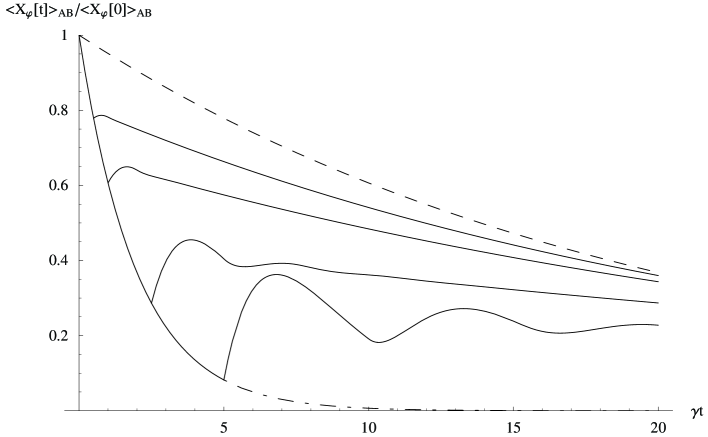
FIG. 1.: Normalized mean value of the measured quadrature $\chi(t)$ (see Eq. (28)) for $g\sin(\theta-\varphi)=0$ (without feedback, dot-dashed line), $g\sin(\theta-\varphi)=0.45$ and some values of the delay time: from bottom to top: $\gamma\tau=5$, $\gamma\tau=2.5$, $\gamma\tau=1$, $\gamma\tau=0.5$ (full lines) and $\gamma\tau=0$ (dashed line).

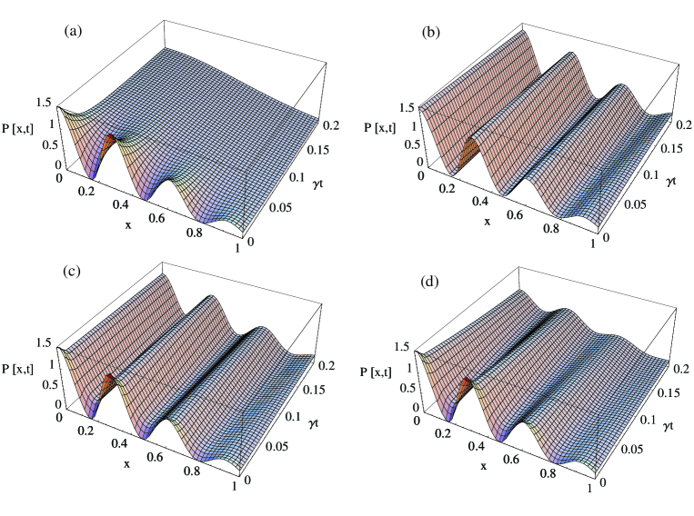
FIG. 2.: Time evolution of the marginal probability distribution $P(x,t)$ ($x=x_{\varphi}$) for the initial state (74) with $\alpha_{0}=i5$. (a) refers to the no feedback case ($g\sin(\theta-\varphi)=0$); (b) refers to the ideal limit of zero feedback delay time and $\eta=1$, with $g\sin(\theta-\varphi)=1$; (c) refers to the case with a non-zero feedback delay time ($\gamma\tau=0.01$) $\eta=1$ and with $g\sin(\theta-\varphi)=1$; (d) refers to the case $\gamma\tau=0.01$, $\eta=0.9$ and $g\sin(\theta-\varphi)=1$.

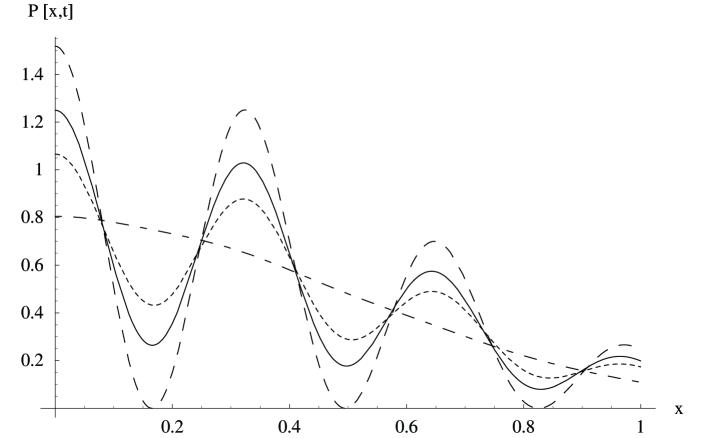
FIG. 3.: Comparison at $\gamma t=0.1$ of the marginal probability distribution $P(x,t)$ between the cases of no feedback (dot-dashed line), feedback with zero delay time ($g\sin(\theta-\varphi)=1$, $\eta=1$, dashed line), feedback with non-zero delay time $\gamma\tau=0.01$ and $\eta=1$ ($g\sin(\theta-\varphi)=1$, full line), and feedback with non-zero delay time and imperfect detection $\gamma\tau=0.01$ and $\eta=0.9$ ($g\sin(\theta-\varphi)=1$, dotted line)

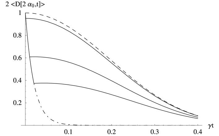
FIG. 4.: Time evolution of $2\langle D(2\alpha_{0},t)\rangle$ for $\alpha_{0}=i5$ and $\varphi=0$ for $g\sin\!\theta=0$ (dot-dashed line), $g\sin\!\theta=1$ with $\gamma\tau=0$ (dashed line) and $g\sin\!\theta=1$ with, from bottom to top, $\gamma\tau=0.02$, $\gamma\tau=0.01$, $\gamma\tau=0.001$ (full lines).

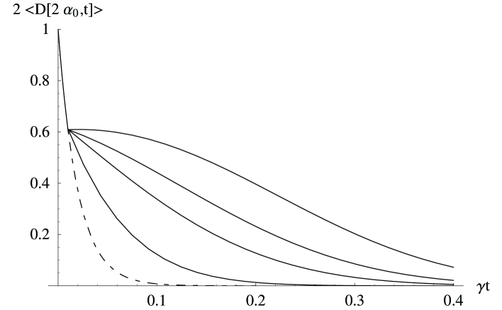
FIG. 5.: Time evolution of $2\langle D(2\alpha_{0},t)\rangle$ for $\alpha_{0}=i5$ and $\varphi=0$ in the presence of feedback with non-zero delay time ($\gamma\tau=0.01$ and $g\sin\!\theta=1$) and for different values of the homodyne detection efficiency $\eta$; from bottom to top, $\eta=0.75$, $\eta=0.9$, $\eta=0.95$, $\eta=1$ (full lines). The dashed line refers to the no-feedback case.

REFERENCES

- [1] H.M. Wiseman and G.J. Milburn, Phys. Rev. Lett. 70, 548 (1993).
- [2] H.M. Wiseman and G.J. Milburn, Phys. Rev. A 49, 1350 (1994).
- [3] H.M. Wiseman, Phys. Rev. A 49, 2133 (1994).
- [4] P. Tombesi and D. Vitali, Phys. Rev. A 50, 4253 (1994).
- [5] P. Tombesi and D. Vitali, Appl. Phys. B 60, S69 (1995); Phys. Rev. A 51, 4913 (1995).
- [6] P. Goetsch, P. Tombesi and D. Vitali, Phys. Rev. A 54, 4519 (1996).
- [7] D. Vitali, P. Tombesi, G.J. Milburn, Phys. Rev. Lett. 79, 2442 (1997).
- [8] S. Mancini, D. Vitali, and P. Tombesi, Phys. Rev. Lett. 80, 688 (1998).
- [9] D. Vitali, P. Tombesi, G.J. Milburn, Phys. Rev. A 57, 4930 (1998).
- [10] J.F. Poyatos, J.I. Cirac and P. Zoller, Phys. Rev. Lett. 77, 4728 (1996).
- [11] A. Ekert and R. Josza, Rev. Mod. Phys 68, 733 (1996).
- [12] B.M. Bay, P. Lambropoulos, and K. Molmer, Phys. Rev. Lett. 79, 2654 (1997).
- [13] L. Diósi, N. Gisin, and W.T. Strunz, Phys. Rev. A 58, 1699 (1998); T. Yu, L. Diósi, N. Gisin, and W.T. Strunz, LANL e-print archive quant-ph/9902043.
- [14] M.W. Jack, M.J. Collett, and D.F. Walls, LANL e-print archive quant-ph/9807028.
- [15] H.J. Carmichael, An Open System Approach to Quantum Optics, Lecture Notes in Physics m18, (Springer, Berlin, 1993).
- [16] M.J. Collett and C.W. Gardiner, Phys. Rev. A 30, 1386 (1984); C.W. Gardiner and M.J. Collett, Phys. Rev. A 31, 3761 (1985).
- [17] C.W. Gardiner Quantum Noise (Springer, Berlin, 1991).
- [18] C.W. Gardiner, A.S. Parkins and P. Zoller, Phys. Rev. A 46, 4363 (1992).
- [19] P. Goetsch and R. Graham, Phys. Rev. A 50, 5242 (1994).
- [20] H.M. Wiseman and G.J. Milburn, Phys. Rev. A 47, 642 (1993).
- [21] K. Jacobs and P.L. Knight, Phys. Rev. A 57, 2301 (1998).
- [22] P. Goetsch, R. Graham and F. Haake, Phys. Rev. A 51, 136 (1995).