Nonclassical fields and the nonlinear interferometer

Abstract

We demonstrate several new results for the nonlinear interferometer, which emerge from a formalism which elegantly describes the output field of the nonlinear interferometer as two-mode entangled coherent states. We clarify the relationship between squeezing and entangled coherent states, since a weak nonlinear evolution produces a squeezed output, while a strong nonlinear evolution produces a two-mode, two-state entangled coherent state. In between these two extremes exist superpositions of two-mode coherent states manifesting varying degrees of entanglement for arbitrary values of the nonlinearity. The cardinality of the basis set of the entangled coherent states is finite when the ratio $\chi/\pi$ is rational, where $\chi$ is the nonlinear strength. We also show that entangled coherent states can be produced from product coherent states via a nonlinear medium without the need for the interferometric configuration. This provides an important experimental simplification in the process of creating entangled coherent states.

I Introduction

The nonlinear interferometer exhibits remarkable properties, even for semiclassical input fields such as a product coherent state, $|\alpha\rangle_{a}|\beta\rangle_{b}$ into the two input ports. Despite the classical nature of the input state, the output state can be highly nonclassical. This nonclassical nature is most apparent in the manifestation of the entangled coherent states. We develop and apply an entangled coherent states formalism to obtain new results. Firstly, we establish the relationship between entangled coherent states and squeezed states, arising from weak nonlinearity, $\chi$, where $\chi$ is proportional to the nonlinear parameter of the medium and to the interaction time in the medium. Strong nonlinearity, in contrast, produces a two-mode, bi-valued entangled coherent state,

$$2^{-1/2}(|0\rangle_{a^{\prime}}|\alpha\rangle_{b^{\prime}}+i|-i\alpha\rangle_{a^{\prime}}|0\rangle_{b^{\prime}}).$$ (1)

In between these two extreme nonlinearities, the output is a general entangled coherent state, which interpolates between the two-mode bi-valued entangled coherent state and the squeezed state. Moreover, for $\chi/\pi$ rational, the output state is a finite sum of product coherent states, and for $\chi/\pi$ irrational, the sum is replaced by an integral. Finally, entangled coherent states can be produced without the need for the interferometer configuration, resulting in a significant simplification for producing entangled coherent states.

The construction of the nonlinear interferometer is achieved by placing a nonlinear optical medium along one internal optical path. For example, a nonlinear medium can be placed in one or both arms of the Mach-Zehnder interferometer [1, 2, 3, 4]. The ideal nonlinear Mach-Zehnder interferometer is mathematically equivalent to other nonlinear two-mode interferometers. Loss and phase diffusion are assumed to be negligible in this treatment.

We treat the nonlinear medium as a classical object which enables photon-photon interactions. The input field at each port is treated as a single-mode field. In Section II, we develop a formal treatment of the interferometer as a unitary transformation of two input states into two output states. In Section III, we discuss the nature of the interferometer and examine special cases and also the case for an arbitrary value of the nonlinearity coefficient $\chi$. In Section IV, we derive the result that a weak value of the nonlinearity coefficient produces squeezed state outputs. In Section V, we show an alternative approach to producing entangled coherent states without using a nonlinear interferometer. In Section VI, we present our conclusions.

II Formalism

The ideal nonlinear interferometer can be described by a unitary transformation of the input fields into the output fields. There are two input fields $a$ and $b$ as shown in Fig. 1, and the output fields are designated by $a^{\prime}$ and $b^{\prime}$. The input fields and output fields are treated as single-mode fields.

For simplicity we consider the special case that the two input fields at the two input ports of the interferometer are coherent states [5] $|\alpha\rangle=\hat{D}(\alpha)|0\rangle$ for

$$\hat{D}(\alpha)=\exp(\alpha\hat{a}^{{\dagger}}-\alpha^{*}\hat{a})$$ (2)

the displacement operator. The coherent field is the closest quantum analogy to the classical coherent field. Its properties include being in a minimum uncertainty state and being generated by a classical current distribution. Coherent field inputs in each arm have proven to be very interesting as these are precisely the inputs considered for squeezing experiments [6] and for obtaining entangled coherent states [7, 8, 9, 10, 11, 12, 13, 14, 15], also regarded as superpositions of multimode coherent states [16, 17, 18, 19]. The unitary transformation operator for the nonlinear interferometer is designated by $\hat{\cal I}$. The transformation is a sequence of a beamsplitter transformation $\hat{\cal B}$ followed by a path difference operator $\hat{\Delta}$ followed by the commuting Kerr transformations in each arm, $\hat{\cal S}_{1}$ and $\hat{\cal S}_{2}$, for which $[\hat{\cal S}_{1},\hat{\cal S}_{2}]=0$, and then a final beamsplitter transformation $\hat{\cal B}$. The net transformation is thus

$$\hat{\cal I}=\hat{\cal B}\hat{\cal S}_{1}\hat{\cal S}_{2}\hat{\Delta}\hat{\cal B}$$ (3)

where $\hat{\cal B}$, $\hat{\cal S}_{1}$ and $\hat{\Delta}$ are discussed below.

The 50/50 beamsplitter transformation is given by [20, 21, 22, 23, 24, 25, 26]

$$\hat{\cal B}=\exp\left(i\pi\left[\hat{a}^{{\dagger}}b+\hat{a}b^{{\dagger}}\right]/4\right).$$ (4)

The Kerr medium transformation in each arm is given by[27, 28]

$$\hat{\cal S}_{i}(\chi;\tau)=\exp\left(-i\tau\hat{a}_{i}^{{\dagger}}\hat{a}_{i}-i\chi_{i}\hat{a}_{i}^{{\dagger}2}\hat{a}_{i}^{2}\right)$$ (5)

where $i=1,2$ and $\hat{a}_{1}=\hat{a}$, $\hat{a}_{2}=\hat{b}$ for transformation $\hat{\cal S}_{i}$, $i=1,2$. The normally-ordered interaction is employed rather than the symmetrically-ordered form also found in the literature. In eq. (5) the nonlinearity coefficient $\chi_{i}$ is proportional to the nonlinear coefficient $\chi^{(3)}$ of the medium and the interaction time within the medium. The delay operator is

$$\hat{\Delta}(\Delta)=\exp(i\Delta\hat{b}^{{\dagger}}\hat{b})$$ (6)

and introduces the linear phase shift which occurs between the arms of the Mach-Zehnder interferometer. For the Sagnac interferometer, $\Delta=0$ and $\chi_{1}=\chi_{2}$ is assumed.

The interferometer output state is $\hat{\cal I}|\alpha\rangle_{a}|\beta\rangle_{b}$. The beamsplitter transformation given in eq. (4) transforms the product coherent state as follows

$$\hat{\cal B}|\alpha\rangle_{a}|\beta\rangle_{b}=|2^{-1/2}(\alpha+i\beta)\rangle_{1}|2^{-1/2}(\beta+i\alpha)\rangle_{2}$$ (7)

for $1$ and $2$ the two beamsplitter output fields. Thus the output state is also a direct product of coherent states at its output given a direct product at the input. In fact this result can be generalised for any semiclassical state. A semiclassical state possesses a well-defined positive-definite Glauber-Sudarshan P-representation[5, 29] which behaves like a probability distribution on phase space. A semiclassical product state input $\hat{\rho}_{a}\otimes\hat{\rho}_{b}$, for $\hat{\rho}_{a}$ the density matrix for state $a$ and similar for the input state for $b$, can be expressed as

$$\hat{\rho}_{a}\otimes\hat{\rho}_{b}=\left[\int\frac{d^{2}\alpha}{\pi}P_{a}(\alpha)|\alpha\rangle_{a}\langle\alpha|\right]\otimes\left[\int\frac{d^{2}\beta}{\pi}P_{b}(\beta)|\beta\rangle_{b}\langle\beta|\right],$$ (8)

where $P_{a}(\alpha)$ and $P_{b}(\beta)$ are the P-representations for the states $\hat{\rho}_{a}$ and $\hat{\rho}_{b}$. The output field from the beamsplitter is given by

$$\hat{\cal B}\rho_{a}\otimes\rho_{b}\hat{\cal B}^{{\dagger}} = \int\frac{d^{2}\alpha}{\pi}P_{a}(\alpha)\int\frac{d^{2}\beta}{\pi}P_{b}(\beta)$$ (10)

$$|2^{-1/2}(\alpha+i\beta)\rangle_{a}\langle 2^{-1/2}(\alpha+i\beta)|\otimes|2^{-1/2}(\beta+i\alpha)\rangle_{b}\langle 2^{-1/2}(\beta+i\alpha)|$$

and a mixture of coherent states entering into a beamsplitter is transformed into the obvious mixture of product coherent states at the output. For nonclassical fields this incoherent mixture of product states does not hold as we shall see.

After the beam is split a path difference between the two arms can be introduced, and this is represented mathematically by the delay operator $\hat{\Delta}$. The delay operator acts on the product coherent state of eq. (7) which leaves the beamsplitter to produce the state

$$\hat{\Delta}\hat{\cal B}|\alpha\rangle_{a}|\beta\rangle_{b}=|2^{-1/2}(\alpha+i\beta)\rangle_{1}|2^{-1/2}e^{i\Delta}(\beta+i\alpha)\rangle_{2}.$$ (11)

A phase shift of $\Delta$ has been effected in arm $2$ relative to arm $1$ of the interferometer.

The nonlinear Kerr transformation (5) transforms the coherent state to[27, 28]

$$|\alpha\rangle^{\chi;\tau}\equiv\hat{\cal S}(\chi)|\alpha\rangle=\exp(-|\alpha|^{2}/2)\sum^{\infty}_{n=0}\frac{(\alpha e^{i(\chi-\tau)})^{n}}{\sqrt{n!}}\exp(-i\chi n^{2})|n\rangle$$ (12)

which is henceforth referred to as a ‘sheared state,’ a term which describes the shearing of the Gaussian Q-function for the coherent state over short times [27, 28]. The rotating frame can be chosen by setting $\tau=0$. (Alternately the frame for which $\tau=\chi$ is also used.) The sheared state $|\alpha\rangle^{\chi;\tau=0}$ is a special case of the generalized coherent states of Titulaer and Glauber [30, 31], which can always be represented as a continuous sum of coherent states [31, 32]. Sheared states in particular have been discussed in this form by Miranowicz et al. [33] and by Gantsog and Tanaś [34], and can be expressed as the superposition

$$|\alpha\rangle^{\chi;\tau=0}=\int_{0}^{2\pi}\frac{d\varphi}{2\pi}f_{\chi}(\varphi)|\alpha e^{i(\chi-\varphi)}\rangle$$ (13)

with

$$f_{\chi}(\varphi)=\sum_{n=0}^{\infty}\exp(in\varphi-i\chi n^{2}).$$ (14)

The phase function exhibits interesting properties and is discussed further in Ref. [35]. For $\chi/\pi$ a rational number the integral (13) becomes a discrete sum over a finite number of coherent states [33].

If $\chi/\pi$ is a rational number then there exists an integer quantity $N$, such that

$$|\alpha\rangle^{\chi;\tau=0}=\sum_{n=1}^{N}c_{n}|\alpha e^{i\pi n/N}\rangle.$$ (15)

This results because the factor $\exp[i\chi n(n-1)]$ in eq. (12) is periodic when $\chi/\pi$ is rational. For $r,s$ integers which are relatively prime and $\chi=2(r/s)\pi$, we observe that

$$\frac{r}{s}n^{2}=\frac{r}{s}(n+N)^{2}\mbox{ mod }1$$ (16)

for $N=s$. If $s$ is not prime, then $N\leq s$ is possible; for example eq. (16) is satisfied by $N=s/2$ for $s$ a multiple of $4$ [35]. For the special case that $\chi=\pi/2$ we have $r=1$, $s=4$, and $N=2$ and we find that

$$|\alpha\rangle^{\chi=\pi/2;\tau=0}=2^{-1/2}\left(e^{-i\pi/4}|i\alpha\rangle+e^{i\pi/4}|-i\alpha\rangle\right).$$ (17)

This superposition state[27, 36] has been discussed in the context of optical analogs to Schrödinger’s cat state [7, 37, 38, 39, 40]. Similar analyses can yield a superposition of phase states [41]. More generally the coefficients of the state (15) are determined by solving the $N$ simultaneous equations [31]

$$\sum_{n=1}^{N}c_{n}e^{2i\pi kn/N}=e^{i\chi k(k-1)}$$ (18)

for $k=0,1,...,N-1$. Using the method of Gantsog and Tanaś [34], this can be solved to determine that

$$c_{n}=\frac{1}{N}\sum_{k=0}^{N-1}\exp[-i2\pi kn/N-i\chi k(k-1)],$$ (19)

where $n=1,2,...,N$.

The output field of the interferometer is given by

$$\hat{\cal I}|\alpha\rangle_{a}|\beta\rangle_{b}=\hat{\cal B}|2^{-1/2}(\alpha+i\beta)\rangle_{1}^{\chi_{1}}|2^{-1/2}e^{i\Delta}(\beta+i\alpha)\rangle_{2}^{\chi_{2}}.$$ (20)

If the states $|2^{-1/2}(\alpha+i\beta)\rangle_{1}^{\chi_{1}}$ and $|2^{-1/2}e^{i\Delta}(\beta+i\alpha)\rangle_{2}^{\chi_{2}}$ are semiclassical then the output could be be written as a product coherent state or a mixture of product coherent states in the way that eq. (10) is written. However the sheared states, despite being generalised coherent states, are not semiclassical states. The nature of the interferometer output states are considered in the next section.

III Output states

In order to analyze the output states of the interferometer, the coherent field with amplitude $\beta$ is now restricted to the vacuum state by setting $\beta=0$. Thus the output state that we wish to consider is given by the formal expression

$$\hat{\cal I}|\alpha\rangle_{a}|0\rangle_{b}=\hat{\cal B}|\alpha/\sqrt{2}\rangle_{1}^{\chi_{1}}|i\alpha/\sqrt{2}\rangle_{2}^{\chi_{2}}.$$ (21)

The sheared state can be expressed as a superposition of coherent states according to expression (12). By substituting this result into eq. (21), we obtain the formal result

$$\hat{\cal I}|\alpha\rangle_{a}|0\rangle_{b} = \int_{0}^{2\pi}\frac{d\varphi_{1}}{2\pi}f_{\chi_{1}}(\varphi_{1})\int_{0}^{2\pi}\frac{d\varphi_{2}}{2\pi}f_{\chi_{2}}(\varphi_{2})$$ (23)

$$|\frac{1}{2}\alpha(e^{i(\chi_{1}-\varphi_{1})}-e^{i(\Delta+\chi_{2}-\varphi_{2})})\rangle_{a^{\prime}}|\frac{1}{2}i\alpha(e^{i(\Delta+\chi_{2}-\varphi_{2})}+e^{i(\chi_{1}-\varphi_{1})}\rangle_{b^{\prime}}.$$

The output state is a superposition of two-mode product coherent states.

The simplest case arises for the linear interferometer for which $\chi_{1}=0=\chi_{2}$. In this case we can show that

$$\hat{\cal I}|\alpha\rangle_{a}|0\rangle_{b}=|\alpha(1-e^{i\Delta})/2\rangle_{a^{\prime}}|i\alpha(1+e^{i\Delta})/2\rangle_{b^{\prime}}$$ (24)

as expected. The output state is unchanged for $\chi_{1}=\pi=\chi_{2}$ and both $\chi_{1}=0=\chi_{2}-\pi$ and $\chi_{1}-\pi=0=\chi_{2}$. A periodic behaviour is evident in $\chi_{1}-\chi_{2}$ parameter space.

The case for which $\chi_{1}=\pi/2$ and $\chi_{2}=0$ is interesting as well. In this case we find that

$$\hat{\cal I}|\alpha\rangle_{a}|0\rangle_{b} = 2^{-1/2}e^{-i\pi/4}[|(\alpha(i-e^{i\Delta})/2\rangle_{a^{\prime}}|i\alpha(i+e^{i\Delta})/2\rangle_{b^{\prime}}$$ (26)

$$+i|-\alpha(i+e^{i\Delta})/2\rangle_{a^{\prime}}|-i\alpha(i-e^{i\Delta})/2\rangle_{b^{\prime}}].$$

For $\Delta=\pi/2$, the entangled coherent state [7, 8, 9, 10, 11, 12, 13, 14, 15]

$$\hat{\cal I}|\alpha\rangle_{a}|0\rangle_{b}=2^{-1/2}e^{-i\pi/4}[|0\rangle_{a^{\prime}}|\alpha\rangle_{b^{\prime}}+i|-i\alpha\rangle_{a^{\prime}}|0\rangle_{b^{\prime}}]$$ (27)

is obtained. However, $\Delta\neq 0$ and therefore this state is not obtained by a Sagnac interferometer in contrast to the entangled state of Ref. [8]. The reason for this difference is the normal ordering of the nonlinear interaction here as opposed to the symmetric ordering used in Ref. [8]. Physically alternate orderings introduce different linear phase shifts.

In fact the more general state (26) can be regarded as entangled as well. A superposition of two mode product coherent states

$$|\alpha_{1}\rangle_{a}|\beta_{1}\rangle_{b}+e^{i\varphi}|\alpha_{2}\rangle_{a}|\beta_{2}\rangle_{b}$$ (28)

is entangled provided that the inner products $|_{a}\langle\alpha_{1}|\alpha_{2}\rangle_{a}|$ and $|_{b}\langle\beta_{1}|\beta_{2}\rangle_{b}|$ are sufficiently small. As the overlap functions for the $a$ and $b$ states of expression (26) are given by

$${}_{a^{\prime}}\langle\alpha(i-e^{i\Delta})/2|-\alpha(i+e^{i\Delta})/2\rangle_{a^{\prime}} = \exp(-|\alpha|^{2}[1-i\cos\Delta]/2)$$ (29)

$$= {}_{b^{\prime}}\langle i\alpha(i+e^{i\Delta})/2|-i\alpha(i-e^{i\Delta})/2\rangle_{b^{\prime}},$$ (30)

the inner products quickly become small as $|\alpha|^{2}\rightarrow\infty$. Consequently the state (26) satisfies the criteria for being an entangled coherent state for all $\Delta$. Thus, although the output state for $\Delta=0$ differs from that of Ref. [8], the output is nevertheless an entangled coherent state.

Another special case for the interferometer arises for $\chi\equiv\chi_{1}=\chi_{2}$ and $\Delta=0$. This restriction corresponds to the case generally used in squeezed light experiments [6]. The output state is given by

$$\hat{\cal I}|\alpha\rangle_{a}|0\rangle_{b} = \int_{0}^{2\pi}\frac{d\varphi}{2\pi}f_{\chi}(\varphi)\int_{0}^{2\pi}\frac{d\varphi^{\prime}}{2\pi}f_{\chi^{\prime}}(\varphi)$$ (32)

$$|2^{-1}\alpha e^{i\chi}(e^{-i\varphi}-e^{-i\varphi^{\prime}}\rangle_{a^{\prime}}|2^{-1}i(e^{-i\varphi^{\prime}}+e^{-i\varphi}\rangle_{b^{\prime}}.$$

For the case that $\chi=\pi/2$, we have

$$\hat{\cal I}|\alpha\rangle_{a}|0\rangle_{b}=\frac{1}{2}(|\alpha\rangle_{a^{\prime}}+|-\alpha\rangle_{a^{\prime}})|0\rangle_{b^{\prime}}+\frac{1}{2}i|0\rangle_{a^{\prime}}(|i\alpha\rangle_{b^{\prime}}+|-i\alpha\rangle_{b^{\prime}}).$$ (33)

This state corresponds to an entanglement of a Schrödinger cat state from port $a^{\prime}$ and a vacuum at port $b^{\prime}$ with a vacuum state from port $a^{\prime}$ and a Schrödinger cat state from port $b^{\prime}$. However the Schrödinger cat state in expression (33) is very different from the Schrödinger cat state in eq. (17). This difference is most evident in the photon number distribution. The photon number distribution of eq. (17) is identical to the distribution of the coherent state $|\alpha\rangle$, but the photon number distribution of the state

$$[2(1+e^{-2|\alpha|^{2}})]^{-1/2}(|\alpha\rangle+|-\alpha\rangle)=\cosh(|\alpha|^{2})\sum_{n=0}^{\infty}\frac{\alpha^{2n}}{\sqrt{(2n)!}}|2n\rangle$$ (34)

is quite different and is a superposition of even photon number states only: hence the nomenclature ‘even coherent states’ [7, 38, 39, 40].

Other interesting features arise for various values of $\chi_{1},\chi_{2}$, and $\Delta$, but the interesting states are special cases of eq. (23). One of these special cases arises for $\chi_{1}/\pi$ and $\chi_{2}/\pi$ rational numbers $2p_{1}/q_{1}$ and $2p_{2}/q_{2}$, for each pair $p_{1}$, $q_{1}$ and $p_{2}$, $q_{2}$ relatively prime integers which are very small. Under this condition the sheared state is a superposition of very few distinguishable coherent states according to the sum (15). That is, for the nonlinearities $\chi_{1}$ and $\chi_{2}$, there exist integers $M$ and $N$ such that

$$|\alpha\rangle^{\chi_{1},\tau=0}=\sum_{m=1}^{M}c_{m}|\alpha e^{i\pi m/M}\rangle,$$ (35)

$$|\alpha\rangle^{\chi_{2},\tau=0}=\sum_{n=1}^{N}c_{n}|\alpha e^{i\pi n/N}\rangle.$$ (36)

By substituting (35) and (36) into the interferometer equation in (21), the interferometer output state is found to be

$$\hat{\cal I}|\alpha\rangle_{a}|0\rangle_{b}=\sum_{m=1}^{M}\sum_{n=1}^{N}c_{m}c_{n}|\alpha(e^{i\pi m/M}-e^{i\pi n/N})/2\rangle_{a^{\prime}}|i\alpha(e^{i\pi m/M}+e^{i\pi n/N})/2\rangle_{b^{\prime}},$$ (37)

where the coefficients $c_{m}$ and $c_{n}$ can be calculated from the application of (19). This shows that the general output state for $\chi_{1}$ and $\chi_{2}$ rational is an entangled coherent state with a finite cardinality for the basis set.

The other interesting parameter regime for $\chi$ corresponds to $\chi/\pi$ a small quantity. This case is important in the squeezed light experiments and is the subject of the next section.

IV Weak nonlinearities and squeezing

The weakly nonlinear interferometer is used for squeezed light [42] experiments and corresponds to small to moderate lengths of nonlinear material in each arm of the interferometer. The quantity $\chi$ can be set to a very small number. Here we wish to see how the formal results established in the previous sections can be used to understand the weakly nonlinear interferometer and the phenomenon of squeezing.

In order to understand the weakly nonlinear Mach-Zehnder interferometer, we must understand the sheared state $|\alpha\rangle^{\chi;\tau}$ for which $\chi$ is small. The sheared state can be expressed as

$$|\alpha\rangle^{\chi;0}\equiv\hat{\cal S}(\chi;0)\hat{D}(\alpha)|0\rangle$$ (38)

for $\hat{\cal S}(\chi;0)$ the shear operator (5) and $\hat{D}(\alpha)$ the displacement operator (2). The unitary operators can be rewritten as

$$\hat{\cal S}(\chi;0)\hat{D}(\alpha)=\hat{D}(\alpha)\exp[-i\chi(\hat{a}^{\dagger}+\alpha^{*})^{2}(\hat{a}+\alpha)^{2}].$$ (39)

Suppose that the photon number $|\alpha|^{2}\rightarrow\infty$ and the nonlinear parameter $\chi\rightarrow 0$ such that $\eta=\chi\alpha^{2}$. Consequently terms in eq. (39) with coefficients of order $\eta/|\alpha|$ and smaller are negligible. Relegating details of the calculation to Appendix A, the state (38) can be approximated by

$$|\alpha\rangle^{\chi;0}\approx\exp(-i\Lambda)\hat{D}(\alpha+\delta)\hat{S}(\varepsilon)\hat{S}(-e^{2i\sigma}\varepsilon)|0\rangle,$$ (40)

where $\hat{S}(\varepsilon)$ is the squeeze operator

$$\hat{S}(\varepsilon)=\exp[(\varepsilon^{*}\hat{a}^{2}-\varepsilon\hat{a}^{\dagger 2})/2],$$ (41)

$\hat{D}(\rho)$ is the displacement operator (2), and $\delta$ and $\Lambda$ are complex functions of $\alpha$ and $\chi$ given by eqns. (A15) and (A16) respectively.

It is evident that the state (40) is a vacuum state which has been squeezed along two different axes, then displaced.

The output state for the weakly nonlinear Mach-Zehnder interferometer is given by (21), which, by using eq. (40), can be approximated by

$$\hat{\cal I}|\alpha\rangle_{a}|0\rangle_{b} \approx e^{-i(\Lambda_{1}+\Lambda_{2})}\hat{\cal B}\hat{D}_{1}(\omega_{1}+\delta_{1})\hat{D}_{2}(\omega_{2}+\delta_{2})$$ (43)

$$\hat{S}_{1}(\varepsilon_{1})\hat{S}_{1}(-e^{2i\sigma_{1}}\varepsilon_{1})\hat{S}_{2}(\varepsilon_{2})\hat{S}_{2}(-e^{2i\sigma_{2}}\varepsilon_{2})|0\rangle_{1}|0\rangle_{2}.$$

where $\omega_{1}=\alpha/\sqrt{2}$ and $\omega_{2}=i\alpha/\sqrt{2}$, and $\Lambda_{i}$, $\delta_{i}$, $\varepsilon_{i}$, and $\sigma_{i}$ (for $i=1,2$) are complex functions of $\alpha$, $\chi_{1}$, and $\chi_{2}$ which are given by eqs. (B5), (B6), (B8), and (B9) respectively in Appendix B.

If $\chi\equiv\chi_{1}=\chi_{2}$, then $\varepsilon_{2}=-\varepsilon_{1}$ and $\sigma_{2}=\sigma_{1}$. In this case, eq. (43) can be calculated to find that

$$\hat{\cal I}|\alpha\rangle_{a}|0\rangle_{b} \approx e^{-i(\Lambda_{1}+\Lambda_{2})}\hat{D}_{a^{\prime}}(\gamma_{1})\hat{D}_{b^{\prime}}(\gamma_{2})$$ (45)

$$\hat{S}_{a^{\prime}}(\varepsilon_{1})\hat{S}_{a^{\prime}}(-e^{2i\sigma_{1}}\varepsilon_{1})\hat{S}_{b^{\prime}}(-\varepsilon_{1})\hat{S}_{b^{\prime}}(e^{2i\sigma_{1}}\varepsilon_{1})|0\rangle_{a^{\prime}}|0\rangle_{b^{\prime}}$$

where $\gamma_{i}$ is a complex function of $\alpha$ and $\chi$ and is given by eq. (B13) (for $i=1,2$).

Thus, when $\chi_{1}=\chi_{2}$, the output state is a product state of the squeezed coherent state at port $a^{\prime}$ and an orthogonally squeezed coherent state at port $b^{\prime}$. If we adopt assumptions about strong coherent fields and weak nonlinearities then the treatment of squeezed coherent states from each port is valid.

It is interesting to note that for $\chi_{1}=\chi_{2}$ the two coherent states enter the two input ports of the interferometer and exit again as two squeezed states. The output state is a product state as well.

V Two-field interaction and Entangled Coherent States

In Section III, it was shown that the nonlinear Mach-Zehnder interferometer with coherent state inputs in general results in an output of entangled coherent states. Here, it is shown that entangled coherent states can also be created using only an ideal Kerr nonlinearity with two coherent state inputs, without the need for an interferometer.

The Kerr transformation for a single field input was given by eq. (5). When two input fields, $1$ and $2$, simultaneously enter into the Kerr cell, the Kerr transformation is given by [43, 44]

$$\hat{\cal S}_{12}(\chi,\tau)=\exp[-i\tau(a_{1}^{\dagger}a_{1}+a_{2}^{\dagger}a_{2})-i\chi(a_{1}^{\dagger 2}a_{1}^{2}+a_{2}^{\dagger 2}a_{2}^{2}+4a_{1}^{\dagger}a_{1}a_{2}^{\dagger}a_{2})].$$ (46)

The term $a_{1}^{\dagger}a_{1}a_{2}^{\dagger}a_{2}$ in the exponential represents the nonlinear two-field interaction which occurs where the two input fields superpose in the nonlinear cell. The effect of this is a phase-shift dependent on the photon numbers of both fields, which leaves the photon number of each field unchanged. This property enables the two-field nonlinear interaction to be used as a quantum non-demolition measurement of photon number [43, 44, 45], where one field provides the signal and the other field is used for the measurement.

A simple form of the entangled coherent state can be obtained by using three nonlinear cells, one for the interaction, preceded by two to cancel the shearing effect on the state in phase space without cancelling the interaction term, as shown in Fig. 2. (The more complicated result when only one nonlinear cell is used is calculated in Appendix C.) The two input coherent states, injected into the pair of nonlinear cells, could in fact be created by directing a single coherent beam into a beamsplitter with a product coherent state output.

In this type of arrangement, the total operator of eq. (46) is then reduced to the form

$$\hat{\cal S}^{\prime}_{12}=\exp(-4i\chi\hat{a}_{1}^{{\dagger}}\hat{a}_{1}\hat{a}_{2}^{{\dagger}}\hat{a}_{2}).$$ (47)

For two coherent state inputs, the output in the Fock state basis is

$$|\alpha,\beta\rangle_{12}^{\chi,0} \equiv \hat{\cal S}^{\prime}(\chi,0)\hat{D}_{1}(\alpha)\hat{D}_{2}(\beta)|0\rangle_{1}|0\rangle_{2}$$ (48)

$$= e^{-(|\alpha|^{2}+|\beta|^{2})/2}\sum_{m=0}^{\infty}\sum_{n=0}^{\infty}\frac{\alpha^{m}\beta^{n}}{\sqrt{m!n!}}e^{-4i\chi mn}|m\rangle_{1}|n\rangle_{2}$$ (49)

which is a generalization of expression (38). This can also be expressed in the coherent state basis as

$$|\alpha,\beta\rangle_{12}^{\chi;\tau=0}=\int_{0}^{2\pi}\frac{d\theta}{2\pi}\int_{0}^{2\pi}\frac{d\varphi}{2\pi}g^{\prime}_{\chi}(\theta,\varphi)|e^{-i\theta}\alpha\rangle_{1}|e^{-i\varphi}\beta\rangle_{2},$$ (50)

with

$$g^{\prime}_{\chi}(\theta,\varphi)=\sum_{p,q=0}^{\infty}\exp(i\theta p+i\varphi q-4i\chi pq).$$ (51)

The output state (50) is an entangled coherent state.

If $\chi/\pi$ is a rational number $2r/s$, a finite entangled sum of coherent states results:

$$|\alpha,\beta\rangle^{\chi;0}=\sum_{m=1}^{N}\sum_{n=1}^{N}c_{mn}|e^{2\pi im/N}\alpha\rangle_{1}|e^{2\pi in/N}\beta\rangle_{2},$$ (52)

where $N=s$ if $r$ and $s$ are relatively prime, and $N<s$ is possible otherwise. The coefficients $c_{mn}$ are found by solving the $N^{2}$ simultaneous equations

$$\sum_{m=1}^{N}\sum_{n=1}^{N}c_{mn}e^{2\pi ikm/N}e^{2\pi iln/N}=e^{-4i\chi mn}.$$ (53)

Solving these equations using an extension of the method of Gantsog and Tanaś [34] gives the result

$$c_{mn}=\frac{1}{N^{2}}\sum_{k=0}^{N-1}\sum_{l=0}^{N-1}\exp[-2i(\pi km/N+\pi ln/N+2\chi kl)].$$ (54)

The factor $\exp(-4i\chi kl)$ in the above expression is the nonlinear interaction term. The presence of this factor means that the general output is an entangled sum of coherent states, unless $2\chi/\pi$ is an integer. In the latter case, $\exp(-4i\chi kl)=1$ and the output will be a product state.

For $\chi=\pi/4$, the resulting output state is

$$|\alpha,\beta\rangle^{\chi;0} = \frac{1}{2}[|\alpha\rangle_{1}(|\beta\rangle_{2}+|-\beta\rangle_{2})+|-\alpha\rangle_{1}(|\beta\rangle_{2}-|-\beta\rangle_{2})]$$ (55)

$$= \frac{1}{2}[(|\alpha\rangle_{1}+|-\alpha\rangle_{1})|\beta\rangle_{2}+(|\alpha\rangle_{1}-|-\alpha\rangle_{1})|-\beta\rangle_{2}].$$ (56)

This is an entangled state, comparable to those in eqs. (28) and (33).

A difference between the entangled coherent state in eq. (56) and the entangled coherent states (28) from the nonlinear interferometer can be seen if one of the input states in eq. (56) is in the vacuum state. If we set $\beta=0$, then the output for the Kerr cell becomes

$$|\alpha,0\rangle_{12}^{\chi;0}=|\alpha\rangle_{1}|0\rangle_{2}$$ (57)

Unlike the entangled coherent states produced in the nonlinear interferometer in eqs. (28) and (33), for a single Kerr cell an entangled coherent state only results when both inputs are not in the vacuum state.

There are a number of advantanges to this new alternative approach to creating entangled coherent states. An interferometer uses nonlinear cells, mirrors, and beam splitters. The approach here, using two coherent inputs into a nonlinear cell, produces entangled coherent states without the need for mirrors or beamsplitters. Thus, many technical difficulties of interferometry are eliminated.

VI Conclusion

The formalism which has been presented here has clarified that for coherent state inputs, the general output of the nonlinear Mach-Zehnder interferometer consists of entangled coherent states. For weak nonlinear evolution, a squeezed state output results. At the other extreme of high values of the nonlinear Kerr coefficient, $\chi=\pi/2$, the entangled coherent state $2^{-1/2}(|0\rangle_{a}|\alpha\rangle_{b}+i|-i\alpha\rangle_{a}|0\rangle_{b})$ results for a single coherent state input into one port of the interferometer, and a vacuum state entering the other port. For states in between these two extremes, in general a type of entangled coherent state will be produced.

It has also been demonstrated that entangled coherent states can also be produced using only an ideal Kerr nonlinearity without the need for an interferometer. For two coherent input states $|\alpha\rangle$ and $|\beta\rangle$ into an ideal Kerr nonlinearity, the interaction between the two states produces the entangled coherent state output $2^{-1}[|\alpha\rangle_{a}(|\beta\rangle_{b}+|-\beta\rangle_{b})+|-\alpha\rangle_{a}(|\beta\rangle_{b}-|-\beta\rangle_{b})]$. While still an entangled state, this entangled state produced by a nonlinear Kerr cell differs from that produced by a nonlinear Mach-Zehnder interferometer since in the former case, both inputs must not be in the vacuum state. If one of the input states is the vacuum state, the other coherent state input passes through unchanged.

A Approximating the Displacement-Shear Unitary Operator

Recall from eq. (39) that

$$\hat{\cal S}(\chi;0)\hat{D}(\alpha)=\hat{D}(\alpha)\exp[-i\chi(\hat{a}^{\dagger}+\alpha^{*})^{2}(\hat{a}+\alpha)^{2}],$$ (A1)

and that we have introduced the quantity

$$\eta=\chi\alpha^{2},$$ (A2)

and we allow $\chi\rightarrow 0$ and $|\alpha|^{2}\rightarrow\infty$ such that $\eta$ remains constant.

Expanding the exponential in (A1) and keeping only those $\alpha$ terms of order 2 or greater produces the result

$$\hat{\cal S}(\chi;0)\hat{D}(\alpha)\approx\hat{D}(\alpha)\exp( -4i|\eta|^{2}\hat{a}^{\dagger}\hat{a}-2i\alpha^{*}\eta\hat{a}^{\dagger}-2i\alpha\eta^{*}\hat{a}$$ (A4)

$$-i\eta\hat{a}^{\dagger 2}-i\eta^{*}\hat{a}^{2}-i\chi|\alpha|^{4}).$$

On the other hand, the term $\hat{S}(\varepsilon)\hat{D}(\alpha)\hat{R}(\rho)\hat{D}^{\dagger}(\alpha)\hat{S}^{\dagger}(\varepsilon)$ can be expanded so that

$$\hat{S}(\varepsilon)\hat{D}(\alpha)\hat{R}(\rho)\hat{D}^{\dagger}(\alpha)\hat{S}^{\dagger}(\varepsilon)$$ (A5)

$$=\exp[i\sigma(\hat{a}^{\dagger}\cosh|\varepsilon|+\hat{a}\frac{\varepsilon}{|\varepsilon|}\sinh|\varepsilon|-\alpha^{*})(\hat{a}\cosh|\varepsilon|+\hat{a}^{\dagger}\frac{\varepsilon^{*}}{|\varepsilon|}\sinh|\varepsilon|-\alpha)].$$ (A6)

Therefore, (A4) can be re-expressed as

$$|\alpha\rangle^{\chi;0}\approx\exp[i\chi|\alpha|^{4}-i\sigma(\sinh^{2}|\varepsilon|+|\alpha|^{2})]\hat{D}(\alpha)\hat{S}(\varepsilon)\hat{D}(\rho)\hat{R}(\sigma)\hat{D}^{\dagger}(\rho)\hat{S}^{\dagger}(\varepsilon)|0\rangle,$$ (A7)

where $\hat{D}(\rho)$ is the displacement operator (2), $\hat{S}(\varepsilon)$ is the squeeze operator (41), and $\hat{R}(\sigma)$ is the rotation operator $\hat{R}(\sigma)=\exp(i\sigma\hat{a}^{\dagger}\hat{a})$, as long as the following simultaneous equations hold:

$$\sigma\cosh 2|\varepsilon|=-4|\eta|^{2}$$ (A8)

$$\sigma\frac{\varepsilon}{|\varepsilon|}\sinh 2|\varepsilon|=-2\eta^{*}$$ (A9)

and

$$\sigma(-\rho^{*}\cosh|\varepsilon|-\rho\frac{\varepsilon}{|\varepsilon|}\sinh|\varepsilon|)=-2\alpha\eta^{*}.$$ (A10)

Solving these equations gives the resultant expressions

$$\rho=\frac{2\alpha^{*}\eta}{\sigma}\cosh|\varepsilon|-\frac{2\alpha\eta^{*}}{\sigma}\frac{\varepsilon^{*}}{|\varepsilon|}\sinh|\varepsilon|;$$ (A11)

$$\varepsilon=\frac{1}{2}\frac{\eta^{*}}{|\eta|}\tanh^{-1}\left(\frac{1}{2|\eta|}\right);$$ (A12)

and

$$\sigma=-4|\eta|^{2}\sqrt{1-\frac{1}{4|\eta|^{2}}}.$$ (A13)

Eq. (A7) can be further simplified to obtain the result

$$|\alpha\rangle^{\chi;0}\approx\exp(-i\Lambda)\hat{D}(\alpha+\delta)\hat{S}(\varepsilon)\hat{S}(-e^{2i\sigma}\varepsilon)|0\rangle,$$ (A14)

where $\delta$ and $\Lambda$ are given by

$$\delta=\cosh|\varepsilon|\rho(1-e^{i\sigma})-(\varepsilon/|\varepsilon|)\sinh|\varepsilon|\rho^{*}(1-e^{-i\sigma});$$ (A15)

and

$$\Lambda=\chi|\alpha|^{4}+\sigma(\sinh^{2}|\varepsilon|+|\alpha|^{2})+|\rho|^{2}\sin\sigma-\mbox{Im}\{\alpha\delta^{*}\}.$$ (A16)

The expression (A14) is obtained by using the relation

$$\hat{R}(\sigma)\hat{D}^{\dagger}(\rho)\hat{S}^{\dagger}(\varepsilon)=\hat{D}^{\dagger}(e^{i\sigma}\rho)\hat{S}^{\dagger}(e^{2i\sigma}\varepsilon)\hat{R}(\sigma)$$ (A17)

as well as the property for the displacement operator [46]

$$\hat{D}(\alpha)\hat{D}(\beta)=\hat{D}(\alpha+\beta)\exp(i\mbox{Im}\{\alpha\beta^{*}\})$$ (A18)

and the commutation relation for $\hat{D}$ and $\hat{S}$ [46] .

B The Output of the Nonlinear Interferometer with a Weak Nonlinearity

The output state for the weakly nonlinear Mach-Zehnder interferometer was given in eq. (43), which was

$$\hat{\cal I}|\alpha\rangle_{a}|0\rangle_{b} \approx e^{-i(\Lambda_{1}+\Lambda_{2})}\hat{\cal B}\hat{D}_{1}(\omega_{1}+\delta_{1})\hat{D}_{2}(\omega_{2}+\delta_{2})$$ (B2)

$$\hat{S}_{1}(\varepsilon_{1})\hat{S}_{1}(-e^{i\sigma_{1}}\varepsilon_{1})\hat{S}_{2}(\varepsilon_{2})\hat{S}_{2}(-e^{2i\sigma_{2}}\varepsilon_{2})|0\rangle_{1}|0\rangle_{2}.$$

In this equation, $\omega_{1}$ and $\omega_{2}$ are given by

$$\omega_{1}=\alpha/\sqrt{2},$$ (B3)

$$\omega_{2}=i\alpha/\sqrt{2},$$ (B4)

and $\Lambda_{i}$ and $\delta_{i}$ are given by

$$\Lambda_{i}=\chi|\omega_{i}|^{4}+\sigma_{i}(\sinh^{2}|\varepsilon_{i}|+|\omega_{i}|^{2})+|\rho_{i}|^{2}\sin\sigma_{i}-\mbox{Im}\{\omega_{i}\delta_{i}^{*}\},$$ (B5)

$$\delta_{i}=\cosh|\varepsilon_{i}|\rho_{i}(1-e^{i\sigma_{i}})-(\varepsilon_{i}/|\varepsilon_{i}|)\sinh|\varepsilon_{i}|\rho^{*}_{i}(1-e^{-i\sigma_{i}}),$$ (B6)

with $\rho_{i}$ given by

$$\rho_{i}=\frac{2\omega_{i}^{*}\eta_{i}}{\sigma_{i}}\cosh|\varepsilon_{i}|-\frac{2\omega_{i}\eta^{*}_{i}}{\sigma_{i}}\frac{\varepsilon^{*}_{i}}{|\varepsilon_{i}|}\sinh|\varepsilon_{i}|,$$ (B7)

and $\varepsilon_{i}$ and $\sigma_{i}$ are given by

$$\varepsilon_{i}=\frac{1}{2}\frac{\eta^{*}_{i}}{|\eta_{i}|}\tanh^{-1}(\frac{1}{2|\eta_{i}|}),$$ (B8)

$$\sigma_{i}=-4|\eta_{i}|^{2}\sqrt{1-\frac{1}{4|\eta_{i}|^{2}}},$$ (B9)

with $\eta_{i}$ given by

$$\eta_{i}=\chi_{i}\omega_{i}^{2}$$ (B10)

for $i=1,2$.

If $\chi\equiv\chi_{1}=\chi_{2}$, then eq. (B2) can be calculated to obtain the result given in eq. (45), which was

$$\hat{\cal I}|\alpha\rangle_{a}|0\rangle_{b} \approx e^{-i(\Lambda_{1}+\Lambda_{2})}\hat{D}_{a^{\prime}}(\gamma_{1})\hat{D}_{b^{\prime}}(\gamma_{2})$$ (B12)

$$\hat{S}_{a^{\prime}}(\varepsilon_{1})\hat{S}_{a^{\prime}}(-e^{i\sigma_{1}}\varepsilon_{1})\hat{S}_{b^{\prime}}(-\varepsilon_{1})\hat{S}_{b^{\prime}}(e^{2i\sigma_{1}}\varepsilon_{1})|0\rangle_{a^{\prime}}|0\rangle_{b^{\prime}}.$$

In eq. (B12), $\gamma_{i}$ is a complex function of $\alpha$ and $\chi$ which is given by

$$\gamma_{i}=\frac{1}{\sqrt{2}}\left[\cosh|\varepsilon_{1}|\Gamma_{i}-\frac{\varepsilon_{1}}{|\varepsilon_{1}|}\Gamma_{i}^{*}\right],$$ (B13)

for $i=1,2$, with

$$\Gamma_{1} = [\cosh|\varepsilon_{1}|(\omega_{1}+\delta_{1})+(\varepsilon_{1}/|\varepsilon_{1}|)(\omega_{1}+\delta_{1})^{*}$$ (B15)

$$+i[\cosh|\varepsilon_{1}|(\omega_{2}+\delta_{2})+(e^{i\sigma_{1}}\varepsilon_{1}/|\varepsilon_{1}|)(\omega_{2}+\delta_{2})^{*}]]/(\sinh^{2}|\varepsilon_{1}|),$$

and

$$\Gamma_{2} = [i[\cosh|\varepsilon_{1}|(\omega_{1}+\delta_{1})+(\varepsilon_{1}/|\varepsilon_{1}|)(\omega_{1}+\delta_{1})^{*}]$$ (B17)

$$+\cosh|\varepsilon_{1}|(\omega_{2}+\delta_{2})+(e^{i\sigma_{1}}\varepsilon_{1}/|\varepsilon_{1}|)(\omega_{2}+\delta_{2})^{*}]/(\sinh^{2}|\varepsilon_{1}|).$$

In the above calculation to obtain eq. (B12), we have used the commutation relationship for $\hat{D}$ and $\hat{S}$ [46], as well as the relationship [47]

$$\hat{B}_{ab}\hat{S}_{a}(\varepsilon)\hat{S}_{b}(-\varepsilon)\hat{D}_{a}(\alpha)\hat{D}_{b}(\beta)$$ (B18)

$$=\hat{S}_{a}(\varepsilon)\hat{S}_{b}(-\varepsilon)\hat{D}_{a}([\alpha+i\beta]/\sqrt{2})\hat{D}_{b}([\beta+i\alpha]/\sqrt{2})\hat{B}_{ab}.$$ (B19)

C Producing Entangled Coherent States with a Single Nonlinear Cell

In Section V, it was demonstrated how entangled coherent states could be produced with three nonlinear cells, without the need for an interferometer. One nonlinear cell is used for the nonlinear interaction, and the other two are used to reverse-shear the state in each output. However, a single nonlinear cell, without the other two reverse-shearing cells, can be used by itself to create entangled coherent states, though the nature of the output state has more complicated representation.

In the Fock state basis, the output from a nonlinear cell with two coherent state inputs can be calculated using the nonlinear transformation in eq. (46). The result is

$$\hat{\cal S}|\alpha\rangle_{1}|\beta\rangle_{2}\Bigr{|}_{\tau=0}=e^{-(|\alpha|^{2}+|\beta|^{2})/2}\sum_{m=0}^{\infty}\sum_{n=0}^{\infty}e^{-i\chi m(m-1)}e^{-i\chi n(n-1)}e^{-4i\chi mn}\frac{\alpha^{m}}{\sqrt{m!}}\frac{\beta^{n}}{\sqrt{n!}}|m\rangle_{1}|n\rangle_{2}.$$ (C1)

The output in eq. (C1) can also be expressed as an superposition of product coherent states. This can be done to obtain the result

$$\hat{\cal S}|\alpha\rangle_{1}|\beta\rangle_{2}\Bigr{|}_{\tau=0}=\int_{0}^{2\pi}\frac{d\theta}{2\pi}\int_{0}^{2\pi}\frac{d\varphi}{2\pi}g_{\chi}(\theta,\varphi)|\alpha e^{i(\chi-\theta)}\rangle_{1}|\beta e^{i(\chi-\varphi)}\rangle_{2},$$ (C2)

where

$$g_{\chi}(\theta,\varphi)=\sum_{p,q=0}^{\infty}\exp[-i(\chi p^{2}-\theta p+\chi q^{2}-\varphi q+4\chi pq)].$$ (C3)

If $\chi/\pi$ is a rational number $2r/s$, then $|\alpha,\beta\rangle^{\chi,\tau=0}$ can be expressed as a finite sum of product coherent states,

$$\hat{\cal S}|\alpha\rangle_{1}|\beta\rangle_{2}\Bigr{|}_{\tau=0}=\sum_{m=1}^{N}\sum_{n=1}^{N}c_{mn}|e^{i2\pi m/N}\alpha\rangle_{1}|e^{i2\pi n/N}\beta\rangle_{2}.$$ (C4)

As was true in eq. (52), $N=s$ if $r$ and $s$ are relatively prime, and $N<s$ is possible otherwise. The coefficients $c_{mn}$ are found by solving the simultaneous equations,

$$\sum_{m=1}^{N}\sum_{n=1}^{N}c_{mn}e^{i2\pi km/N}e^{i2\pi ln/N}=e^{-i\chi[k(k-1)+l(l-1)+4kl]},$$ (C5)

for $k,l=0,1,...,N-1$. This gives the result

$$c_{mn}=\frac{1}{N^{2}}\sum_{k=0}^{N-1}\sum_{l=0}^{N-1}\exp[-i2\pi(km+ln)/N-i\chi(k(k-1)+l(l-1)+4kl)].$$ (C6)

If $2\chi/\pi$ is an integer, the output will be a product state, otherwise the output will be an entanglement of coherent states.

When $\chi=\pi/2$, we expect the output to be a product state. Using eqs. (C4) and (C6) yields the product state

$$\hat{\cal S}(\pi/2,0)\hat{D}_{1}(\alpha)\hat{D}_{2}(\beta)|0\rangle_{1}|0\rangle_{2}=-\frac{i}{2}(|i\alpha\rangle_{1}+i|-i\alpha\rangle_{1})(|i\beta\rangle_{2}+i|-i\beta\rangle_{2}).$$ (C7)

For the case of a single nonlinear cell, the simplest entangled coherent state output is obtained for $\chi=\pi/4$:

$$\hat{\cal S}(\pi/4,0)\hat{D}_{1}(\alpha)\hat{D}_{2}(\beta)|0\rangle_{1}|0\rangle_{2}$$ (C8)

$$=\frac{1}{4}[i(|\alpha\rangle_{1}-|-\alpha\rangle_{1})(|\beta\rangle_{2}-|-\beta\rangle_{2}-e^{i\pi/4}|i\beta\rangle_{2}-e^{i\pi/4}|-i\beta\rangle_{2})$$ (C9)

$$+e^{-i\pi/4}(|i\alpha\rangle_{1}+|-i\alpha\rangle_{1})(|\beta\rangle_{2}-|-\beta\rangle_{2}+e^{i\pi/4}|i\beta\rangle_{2}+e^{i\pi/4}|-i\beta\rangle_{2})].$$ (C10)

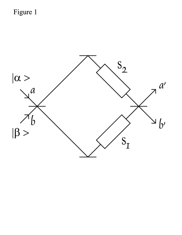
FIG. 1.: Nonlinear Mach–Zehnder interferometer. Coherent states $|\alpha\rangle$ and $|\beta\rangle$ are injected into the two input ports of a beam splitter (BS). where they pass through a nonlinear medium. The fields are then recombined at the second BS.

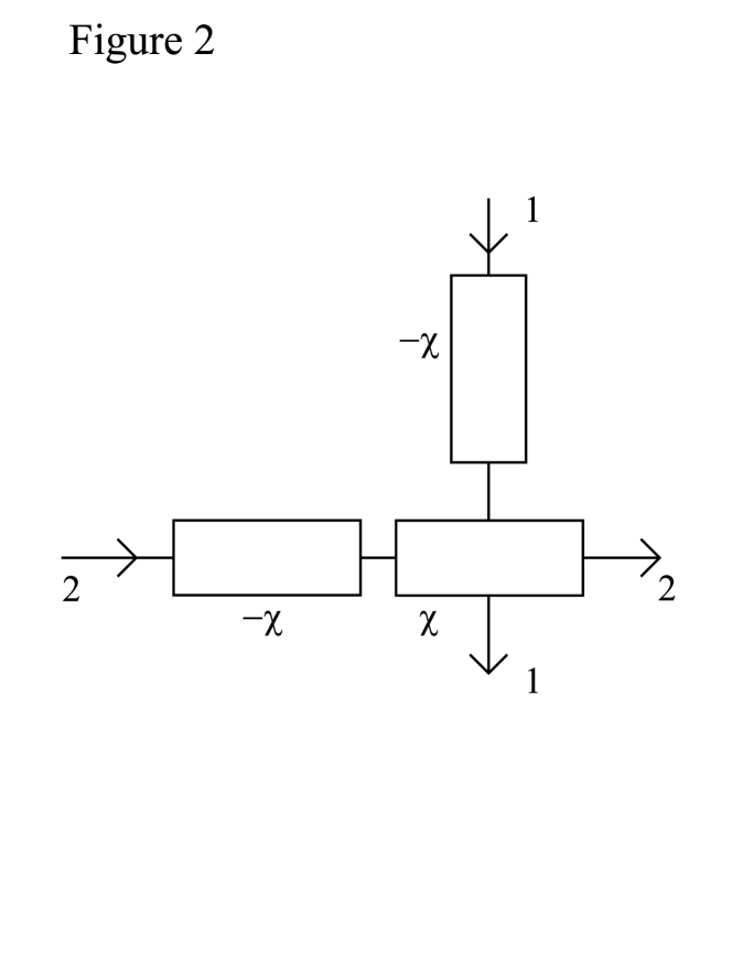
FIG. 2.: Three nonlinear media elements used to create an entangled coherent state.

REFERENCES

• [1] M. Kitagawa and Y. Yamamoto, Phys. Rev. A 34, 3974 (1986).
• [2] M. Shirasaki and H. A. Haus, J. Opt. Soc. Am. B 7, 30 (1990).
• [3] G. J. Milburn, Phys. Rev. Lett62, 2124 (1989).
• [4] H. A. Haus and F. X. Kärtner, Phys. Rev. A 46, R1175 (1992).
• [5] R. J. Glauber, Phys. Rev131, 2766 (1963).
• [6] G. J. Milburn, M. D. Levenson, R. M. Shelby, S. H. Perlmutter, R. G. Devoe, and D. F. Walls, J. Opt. Soc. Am. B 4, 1476 (1987).
• [7] B. C. Sanders, Phys. Rev. A 45, 6811 (1992); 46, 2966 (1992).
• [8] B. Wielinga and B. C. Sanders, J. Mod. Opt40, 1923 (1993).
• [9] A. Mann, B. C. Sanders, and W. J. Munro, Phys. Rev. A 51, 989 (1995).
• [10] B. C. Sanders, K. S. Lee, and M. S. Kim, Phys. Rev. A 52, 735 (1995).
• [11] I. Jex, P. Törmä, and S. Stenholm, J. Mod. Opt42, 1377 (1995).
• [12] C. C. Gerry, Phys. Rev. A 55, 2478 (1997).
• [13] Guang-Can Guo and Shi-Biao Zheng, Opt. Comm133, 142 (1997).
• [14] D. A. Rice and B. C. Sanders, Quant. Class. Opt10, L41 (1998).
• [15] B. C. Sanders and D. A. Rice, Optical and Quantum Electronics 31, 525 (1999).
• [16] P. Tombesi and A. Mecozzi, J. Opt. Soc. Am. B 4, 1700 (1987).
• [17] Chin-Lin Chai, Phys. Rev. A 46, 7187 (1992).
• [18] N. A. Ansari and V. I. Man’ko, Phys. Rev. A 50, 1942 (1994).
• [19] V. V. Dodonov, V. I. Man’ko, and D. E. Nikonov, Phys. Rev. A 51, 3328 (1995).
• [20] H. P. Yuen and J. H. Shapiro, IEEE Trans. Inf. Theory IT-26, 78 (1980).
• [21] M. Ley and R. Loudon, Opt. Commun54, 317 (1985).
• [22] H. Fearn and R. Loudon, Opt. Commun64, 485 (1987).
• [23] Z. Y. Ou, C. K. Hong, and L. Mandel, Opt. Commun63, 118 (1987).
• [24] R. A. Campos, B. E. A. Saleh, and M. C. Teich, Phys. Rev. A 40, 1371 (1989).
• [25] R. Loudon, Coherence and Quantum Optics 6, eds. J. H. Eberly, L. Mandel, and E. Wolf (Plenum Press, New York, 1989), p. 703.
• [26] W. K. Lai, V. Buz̆ek, and P. L. Knight, Phys. Rev. A 43, 6323 (1991).
• [27] G. J. Milburn, Phys. Rev. A 33, 674 (1986).
• [28] G. J. Milburn and C. A. Holmes, Phys. Rev. Lett56, 2237 (1986).
• [29] E. C. G. Sudarshan, Phys. Rev. Lett10, 277 (1963).
• [30] U. M. Titulaer and R. J. Glauber, Phys. Rev145, 1041 (1966).
• [31] Z. Bialynicka-Birula, Phys. Rev173, 1207 (1968).
• [32] D. Stoler, Phys. Rev. D 4, 2309 (1971).
• [33] A. Miranowicz, R. Tanaś, and S. Kielich, Quant. Opt2, 253 (1990).
• [34] Ts Gantsog and R. Tanaś, Quant. Opt3, 33 (1991).
• [35] M. V. Berry and J. Goldberg, Nonlinearity 1, 1 (1988).
• [36] B. Yurke and D. Stoler, Phys. Rev. Lett57 13 (1986).
• [37] E. Schrödinger, Naturwissenschaften 23, 812 (1935).
• [38] J. Per̆ina, Quantum Statistics of Linear and Nonlinear Optical Phenomena (Dordrecht, Reidel, 1984), p. 78.
• [39] M. Hillery, Phys. Rev. A 36, 3796 (1987).
• [40] V. Buz̆ek, A. Vidiella-Barranco, and P. L. Knight, Phys. Rev A. 145, 6570 (1992).
• [41] B. C. Sanders, Phys. Rev. A 45, 7746 (1992).
• [42] R. Loudon and P. L. Knight, J. Mod. Opt34, 709 (1987).
• [43] P. Alsing, G. J. Milburn, and D. F. Walls, Phys. Rev. A 37, 2970 (1988).
• [44] H.-A. Bachor, M. D. Levenson, D. F. Walls, S. H. Permutter, and R. M. Shelby, Phys. Rev. A 38, 180 (1988).
• [45] B. C. Sanders and G. J. Milburn, Phys. Rev. A 39, 694 (1989).
• [46] D. F. Walls and G. J. Milburn, Quantum Optics (Springer-Verlag, Berlin, 1994).
• [47] M. S. Kim and B. C. Sanders, Phys. Rev. A 53, 3694 (1996).
Refer to caption