Does the quantum collapse make sense?
Quantum Mechanics vs Multisimultaneity
in interferometer-series experiments

Abstract

It is argued that the three assumptions of quantum collapse, ‘one photon-one count’, and relativity of simultaneity cannot hold together: nonlocal correlations may depend on the referential frames of the beam-splitters but not of the detectors. New experiments using interferometers in series are proposed which make it possible to test Quantum Mechanics vs Multisimultaneity.

Keywords: multisimultaneity, relativistic nonlocal causality, wavefunction collapse, superposition principle.

1 Introduction

Multisimultaneity (or Relativistic Nonlocality) is a description of physical causality which unifies the relativity of simultaneity and superluminal nonlocality avoiding superluminal signaling. The description accounts in particular for the superluminal nonlocal influences, and the consequent violation of relativistic causality, happening in Bell experiments with space-like separated measuring devices. Multisimultaneity deviates from Quantum Mechanics in that two-particle correlations are supposed to depend on the timing of the arrivals of the particles at the measuring devices. Whereas both theories agree for all experiments conducted so far, they conflict with each other in their predictions regarding new proposed experiments with measuring devices in motion [1, 2, 3, 4].

Work to perform such experiments is in progress [5, 6]. To test for Multisimultaneity it is crucial to set in motion precisely those objects where take place the events which are connected by superluminal influences. The already published work [1, 2, 3] assumes that these events are the arrivals of photons at beam-splitters, and, consequently, what determines the timing is the state of motion and the position of the beam-splitters. As pointed out in [1, 2] there is experimental evidence against the hypothesis that the choice of the output port by which one photon leaves a beam splitter depends on which detector the other photon reaches. However, a version of Multisimultaneity assuming nonlocal causal links between the detectors seems also to be possible in principle, and would have the advantage of keeping the key role that standard Quantum Mechanics attributes to detection.

In this paper we describe an experiment involving pairs of entangled photons running through a series of interferometers (Fig.1). It is shown that a theory assuming both the ‘one photon-one count’ principle (the detection of only one photon cannot produce more than one count) and the relativity of simultaneity has to give up the quantum collapse, and cannot invoke frame-dependent links between detections to explain the correlations. The alternative explanation by means of influences between the beam-splitters allow us within Multisimultaneity to propose new interesting experiments with devices in motion. But it also implies the possibility of producing so called two non-before impacts [2], one at each arm of the setup, with beam-splitters at rest. It is argued that such an experiment may allow us to decide between Multisimultaneity and timing insensitive theories such as Quantum Mechanics without having to set devices in motion. It is also highlighted that the inadequacy of causal links between detections challenges the concept of backward causation.

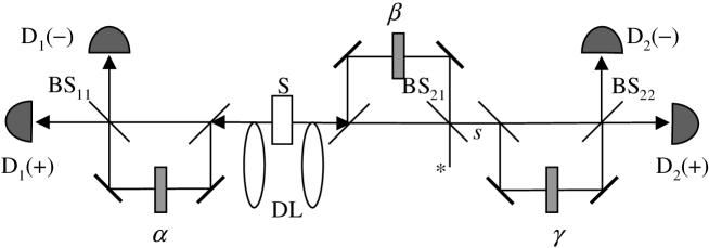
Figure 1: Impact series experiment with photon pairs: photon 2 enters a two interferometer series impacting successively on beam-splitter BS₂₁ and BS₂₂. See text for detailed description.

2 The experiment

Consider the setup sketched in Fig.1. Energy-time entangled photon pairs are emitted from a pulsed source S of the type described in [7]. Photon 1 enters the left interferometer and impacts successively on two beam-splitters before being detected in either D${}_{1}(+)$ or D${}_{1}(-)$ after leaving beam-splitter BS₁₁. Photon 2 enters a first interferometer on the right: if it leaves BS₂₁ by output port $s$ it enters a second interferometer and gets detected in either D${}_{2}(+)$ or D${}_{2}(-)$ after impacting beam-splitter BS₂₂. Each interferometer, also the preparation one within the source [7] (not sketched in Fig. 1), consists in a long arm of length $L$, and a short one of length $l$. We assume the path difference set to a value which largely exceeds the coherence length of the photon pair light, and all beam-splitters to be 50-50 ones.

We label the path pairs leading to detection as follows: $(l,lsl)$; $(L,lsl)$; $(l,Lsl)$ and so on; where, e.g., $(l,Lsl)$ indicates the path pair in which photon 1 has taken the short arm, and photon 2 has taken first the long arm, then the short one. We distribute the ensemble of the 8 possible paths in the four following subensembles:

$$\begin{array}[]{lll}(l,LsL)&:&2L-l\\ (L,LsL)\,,\,(l,Lsl)\,,\,(l,lsL)&:&L\\ (l,lsl)\,,\,(L,Lsl)\,,\,(L,lsL)&:&l\\ (L,lsl)&:&2l-L\end{array}$$ (1)

where the right-hand side of the table indicates the relevant parameter characterizing each subensemble of paths.

Time-resolved detection [8, 9, 10] of the photon pairs cannot distinguish between the paths of subensemble $L$ because all of them will exhibit the same time difference in the detected photon pair signals. Neither can measurement of the time of emission of the pump laser light distinguish between these paths when, as assumed, the path difference $L-l$ between the long and the short path is the same for each interferometer included the preparation one [7]. Therefore according to quantum mechanics the paths of subensemble $L$ will interfere with each other, and the same holds for the paths of subensemble $l$.

On the contrary, time-resolved detection allows us to discriminate between paths of different subensembles in table 1, and in particular between the cases where a pair follows a path of subensemble $L$, and the cases where the pair follows a path of subensemble $l$. A time delay spectrum of coincidence counts [8, 10] for each of the four possible outcomes D${}_{1}(\sigma)$, D${}_{2}(\omega)$  ($\sigma,\omega\in\{+,-\}$) will exhibit four peaks: an interference peak corresponding to subensemble $L$ we suppose set at time difference 0, a second interference peak at time difference $(l-L)/c$ corresponding to subensemble $l$, and two other peaks at time differences $(L-l)/c$ and $(2l-2L)/c$ corresponding to subensemble $2L-l$, respectively $2l-L$. Using a time difference window one can select only the events corresponding to subensemble $L$, or only those to subensemble $l$.

For the sake of simplicity we refer to the different subpopulations of detected photon pairs as subpopulation $L$, $l$ etc. Unless stated otherwise, the experiments considered in the following are supposed to involve only pairs of subpopulation $L$.

By means of delay lines DL different timings can be arranged in the laboratory frame. The beam-splitters can also be supposed as in motion, like in the experiments proposed in [1, 2].

3 Timing insensitive Quantum Mechanics

The quantum mechanical superposition principle states independently of any possible timing:

$$P^{QM}(\sigma,\omega) = \left|A(L\,\sigma,LsL\,\omega)+A(l\,\sigma,Lsl\,\omega)+A(l\,\sigma,lsL\,\omega)\right|^{2}$$ (2)

where $P^{QM}(\sigma,\omega)$ denotes the joint probability of getting the outcome D${}_{1}(\sigma)$, D${}_{2}(\omega)$ in experiments with pairs of subpopulation $L$, and $A(path\,\sigma,path\,\omega)$ the corresponding probability amplitudes for the path and outcome pairs specified within the parentheses.

Substituting the amplitudes into Eq. (2) yields the following values for the conventional joint probabilities:

$$P^{QM}(\sigma,\omega)=\frac{1}{64}\Big{[}3+\sigma\,2\cos(\alpha+\beta)+2\sigma\omega\,\cos(\alpha+\gamma)+\omega\,2\cos(\gamma-\beta)\Big{]}$$ (3)

From (3) one is led to the following usual correlation coefficient:

$$E^{QM}_{\sigma\omega}=\frac{\sum_{\sigma,\,\omega}\sigma\omega\,P^{QM}(\sigma,\omega)}{\sum_{\sigma,\,\omega}P^{QM}(\sigma,\omega)}=\frac{2}{3}\cos(\alpha+\gamma)$$ (4)

and the special ones:

$$E^{QM}_{\sigma}=\frac{\sum_{\sigma,\,\omega}\sigma\,P^{QM}(\sigma,\omega)}{\sum_{\sigma,\,\omega}P^{QM}(\sigma,\omega)}=\frac{2}{3}\cos(\alpha+\beta)$$ (5)

$$E^{QM}_{\omega}=\frac{\sum_{\sigma,\,\omega}\omega\,P^{QM}(\sigma,\omega)}{\sum_{\sigma,\,\omega}P^{QM}(\sigma,\omega)}=\frac{2}{3}\cos(\gamma-\beta)$$ (6)

Moreover, from Eq. (3) one is led to the relation:

$$P^{QM}(\sigma,\pm)=\sum_{\omega}P^{QM}(\sigma,\omega)=\frac{1}{32}\Big{[}3+\sigma\,2\cos(\alpha+\beta)\Big{]}$$ (7)

where $P^{QM}(\sigma,\,\pm)$ denotes the probability of getting photon 1 detected in D${}_{1}(\sigma)$ independently of where photon 2 is detected, for experiments with pairs of subpopulation $L$, or in other words, the probability of getting a pair reaching BS₁₁ and BS₂₂ by a path of subpopulation $L$, and photon 1 detected in D${}_{1}(\sigma)$.

4 Sharp defined relativistic nonlocal causal links

As far as one looks upon correlated events as revealing some kind of influence at work (“correlations cry out for explanation,” John Bell said), three kinds of sharp defined frame-dependent causal links can be considered candidates to explain the correlations:

1. Detection-detection: The choice of the detector into which photon $i$ falls influences the choice of the detector into which photon $j$ falls.

2. Detection-splitter: The detection of photon $i$ influences the choice of the output port by which photon $j$ leaves a beam-splitter.

3. Splitter-splitter: The choice of the output port by which photon $i$ leaves the beam-splitter influences the choice of the output port by which photon $j$ leaves a beam-splitter.

4.1 Relativistic nonlocal influences between detections contradict the ‘one photon-one count’ principle

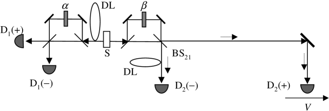
Figure 2: Experiment with detectors D${}_{2}(\omega)$ in relative motion to each other. See text for detailed description.

Consider the simplified experiment sketched in Fig. 2 in which each photon runs through only one interferometer, and assume that the detection of photon 2 occurs time-like separated before the detection of photon 1. The hypothesis that till the instant of detection it is not determined which of the two detectors D${}_{2}(\omega)$ fires necessarily implies some kind of superluminal influence or Bell connection between these detectors. Suppose that D${}_{2}(+)$ and D${}_{2}(-)$ are set in relative motion to each other so that the arrival of photon 2 at any D${}_{2}(\omega)$, in the inertial frame of D${}_{2}(\omega)$, occurs before the arrival of photon 2 to D${}_{2}(-\omega)$. Under these conditions, the fact that D${}_{2}(\omega)$ fires, cannot depend on whether D${}_{2}(-\omega)$ fires or not, and therefore it should happen that $25\%$ of the times D${}_{2}(+)$ and D${}_{2}(-)$ fire together even if there is only one particle traveling the right side of the setup, and $25\%$ of the times neither D${}_{2}(+)$ nor D${}_{2}(-)$ fires when photon 2 reaches these detectors. This clearly contradicts the basic ‘one photon-one count’ principle. Therefore, as far as one keeps this principle and the relativity of simultaneity, one has to reject that the outcomes are determined by relativistic nonlocal connections between D${}_{2}(+)$ and D${}_{2}(-)$, and accept they are determined when the particles leave the beam-splitters. Notice that this conclusion also holds for single particle experiments. Moreover, the conclusion obviously implies that each particle consists of a detectable part leaving the splitter by one of the output ports, and an undetectable part leaving by the other.

In summary, realtivistic nonlocal causal links between detectors seem inadequate to explain the correlations.

4.2 Experiment rules out detection-splitter links

Even if the outcomes are determined when the particles leave the beam-splitters, as stated in Subsection 4.1, one could nevertheless imagine that the correlations appear because the detection of particle $j$ affects the outcome choice of particle $i$ at the corresponding beam-splitter.

Suppose a conventional Bell-experiment with detectors set at distances such that the detection of each particle lies always time-like separated after the arrival of the other particle at the beam-splitter. As referred to in [1], the experiment used in [11] fulfills this condition.

For such an experiment, the considered detection-splitter hypothesis would imply the disappearance of the correlations, for none of the particles can be affected by any influence from the other side. The experimental results in [11] contradict this prediction, and rule out the hypothesis that the correlations arise because detection-splitter links.

4.3 Splitter-splitter links, the remaining explanation

In conclusion, any causal explanation sharing the ‘one photon-one count’ principle and the relativity of simultaneity has to assume that what matters for the appearance of correlations are frame-dependent links between events at the beam-splitters. Detection only reveals choices which have taken place already, and does not play any particular role in determining which outcome occurs.

5 Timing-dependent Multisimultaneity

In agreement with the conclusions of Section 4 Multisimultaneity assumes that the outcome of an experiment depends on the relative state of motion and position of the beam-splitters in which interferences take place, and not of the detectors, for instance, in the experiment of Fig.1, the beam-splitters BS₁₁, BS₂₁, and BS₂₂. Then, arbitrary large series of interferometers make it possible to arrange plenty of different timings, beyond the three already discussed in the realm of conventional Bell setups, i.e., two before, one non-before, and two non-before Timings [1, 2], and obviously Multisimultaneity has to account for all of them.

5.1 Principles of Multisimultaneity

First of all we generalize the main concepts and principles in [1, 2] in order to describe experiments with series of interferometers.

We assume that each particle $i$ consists of an observable or detectable part traveling by one of the paths, and several unobservable parts traveling by the other possible paths at the same speed as the observable one. Moreover we assume that the impacts of the observable parts of the two photons on the beam-splitters are connected by means of superluminal influences.

We denote $(T_{jl})_{ik}$ ($i,j\in\{1,2\};k,l\in\{1,2...n\}$) the time at which the observable part of particle $j$ impacts on beam-splitter BS_jl, measured in the inertial frame of BS_ik (the subscript $ik$ after a parenthesis means all times within the parentheses to be measured in the inertial frame of BS_ik).

At time $(T_{ik})_{ik}$, we consider the latest BS_jl, if any, such that $(T_{jl}\leq T_{ik})_{ik}$. If at any time $T$ such that $(T_{ik}<T<T_{i\,k+1})_{ik}$ and $(T_{jl}<T<T_{j\,l+1})_{ik}$, it is impossible to distinguish by which path the particles did travel before leaving the beam-splitters BS_ik and BS_jl, the impact on BS_ik is said to be non-before the impact on BS_jl, and denoted $a_{ik[jl]}$, or simply $a_{ik}$ if no ambiguity results. Otherwise, the impact on BS_ik is called a before one, and denoted $b_{ik}$. Expressions like $a_{ik[jl]\,\sigma}$, $b_{ik\,\sigma}$ denote that the detectable part of particle $i$ leaves BS_ik by the output port $\sigma$ in the indicated non-before, respectively beforeimpact. One could say that a photon undergoing a non-before impact can consider, from “its point of view”, indistinguishability guaranteed if detections occur, and a photon undergoing a before impact cannot.

According to these definitions, the conventional Bell tests are referred to as $(b_{i},a_{j})$ experiments, for all beam-splitters are at rest, and one of the impacts always occurs before the other in the laboratory frame. The Timing considered in Section 4 is referred to as $(b_{11},a_{21}\,a_{22})$. Besides this Timing, we will be interested in the following two other ones: $(b_{11},b_{21}\,a_{22})$, and $(a_{11[21]},b_{21}\,a_{22})$.

Multisimultaneity rests on two main principles:

1. Principle I: Values $b_{ik\,\sigma}$ do not depend on phase parameters particle $j$ meets.

2. Principle II: Values $a_{ik[jl]\,\sigma}$ do not depend on values $a_{jl^{\prime}[ik^{\prime}]\,\omega^{\prime}}$ ($l^{\prime}\leq l$) particle $j$ may actually produce, but only of the values $b_{jl^{\prime}\,\omega}$ particle $j$ would have produced in corresponding before impacts.

Because of the Bell experiments already conducted, Principle II obviously implies that in experiments $(b_{i},a_{j})$ the distribution of the outcome results is calculated combining the amplitudes of the single alternative paths, the same way as Quantum Mechanics does. This rule is extended to experiments in which all the impacts of particle $i$ are before, and all those of particle $j$ are non-before, i.e., in such experiments the conventional Quantum Mechanical rule of combining amplitudes applies. Regarding experiments like $(b_{11},b_{21}\,a_{22})$ in which particle $i$ undergoes only before impacts, and particle $j$ undergoes some before and some non-before ones, the outcome’s distribution is still calculated combining amplitudes, but according rules unknown in Quantum Mechanics, as we will see in Subsection 5.3.

In experiments involving an $a_{ik[jl]}$ impact and an $a_{jl^{\prime}[ik]}$ one, it would be absurd to assume together that the impacts on BS_ik take into account the actual outcomes of the impacts on BS${}_{jl^{\prime}}$, and that the impacts on BS${}_{jl^{\prime}}$ take into account the actual outcomes of the impacts on BS_ik. Therefore, Timing $(a_{11[22]},b_{21}a_{22})$ requires that $a_{11[22]\,\sigma}$ depends on $b_{21}b_{22\,\omega^{\prime}}$, and $b_{21}a_{22\,\omega}$ on $b_{11\,\sigma^{\prime}}$; Timing $(a_{11[22]},a_{21}a_{22})$ that $a_{11\,\sigma}$ depends either on $b_{21\,\ast}$, or on $b_{21\,s\,l}$, or on $b_{21}b_{22\,\omega^{\prime}}$, and $a_{21}a_{22\,\omega}$ depends on $b_{11\,\sigma^{\prime}}$. The motivation of Principle II is to account for all Timings involving non-before impacts without multiplying hypothesis needlessly.

Assuming the relativity of simultaneity and excluding backward causation, Multisimultaneity consequently forbids superluminal signaling. This impose constraints to the path amplitudes. It implies in particular that for any non-selective experiment the probability that particle $i$ produces the result $\sigma$ (independently of which outcome particle $j$ produces) does not depend on timing.

5.2 Timing $(b_{11},a_{21}\,a_{22})$

Such a Timing can be easily arranged by keeping all beam-splitters at rest, at distances such that the impact on BS₁₁ occurs before the impact on BS₂₁.

Regarding the pairs whose detectable parts travel path $(l,L)$, photon 2 at its arrival at BS₂₁ cannot consider indistinguishability guaranteed, and therefore the probability of getting photon 1 detected in D${}_{1}(\sigma)$, and the detectable part of photon 2 leaving BS₂₁ by output port $s$ is given by the relation:

$$P(b_{11\,\sigma},b_{21\,s})=P(l,L)P(b_{11\,\sigma}|l,L)P(b_{21\,s}|l,L)$$ (8)

where $P(l,L)$ means the probability of having a pair with detectable parts traveling path $(l,L)$, $P(b_{11\,\sigma}|l,L)$ the probability that photon 1’s detectable part of such a pair leaves BS₁₁ by output port $\sigma$, and $P(b_{21\,s}|l,L)$ the probability that photon 2’s detectable part leaves BS₂₁ by output port $s$. Therefore it holds that:

$$P(b_{11\,\sigma},b_{21\,s})=\frac{1}{2^{2}}\frac{1}{2}\frac{1}{2}=\Big{|}A(l\,\sigma,Ls)\Big{|}^{2}=\frac{1}{2^{4}}$$ (9)

Consider now the pairs whose detectable parts travel one of the paths $(L,L)$ or $(l,l)$. Since photon 2 at its arrival at BS₂₁ can consider indistinguishability guaranteed, the probability of getting photon 1 detected in D${}_{1}(\sigma)$, and the detectable part of photon 2 leaving BS₂₁ by output port $s$ is given by the relation:

$$P(b_{11\,\sigma},a_{21\,s}) = P(l,l)P(b_{11\,\sigma}|l,l)P(a_{21\,s}|b_{11\,\sigma})$$ (10)

$$+ P(L,L)P(b_{11\,\sigma}|L,L)P(a_{21\,s}|b_{11\,\sigma})$$

where $P(a_{21\,s}|b_{11\,\sigma})$ denotes the probability that in a pair undergoing impacts $(b_{11},a_{21})$ photon 2’s observable part leaves BS₂₁ by output port $s$, assuming photon 1’s observable part did leave BS₁₁ by output port $\sigma$. We assume this conditional probability to be given by the relation:

$$P(a_{21\,s}|b_{11\,\sigma}) = \frac{|A(L\,\sigma,L\,s)+A(l\,\sigma,l\,s)|^{2}}{\sum_{\omega}|A(L\,\sigma,L\,\omega)+A(l\,\sigma,l\,\omega)|^{2}}\vspace{0.2cm}$$ (11)

$$= \frac{1}{2}[1+\sigma\,\cos(\alpha+\beta)]$$

Substituting (11) into (10) one gets:

$$P(b_{11\,\sigma},a_{21\,s}) = \Big{|}A(L\,\sigma,Ls)+A(l\,\sigma,ls)\Big{|}^{2}$$ (12)

$$= \frac{1}{2^{4}}\Big{[}2+\sigma\,2\cos(\alpha+\beta)\Big{]}$$

From Eq. (12) and (9) it follows that the probability of a pair reaching BS₁₁ and BS₂₂ by a path of subpopulation $L$, and producing outcome D${}_{1}(\sigma)$ is given by the relation:

$$P(b_{11\,\sigma},a_{21}\,a_{22\,\pm}) = \frac{1}{2}\Big{|}A(L\,\sigma,Ls)+A(l\,\sigma,ls)\Big{|}^{2}+\frac{1}{2}\Big{|}A(l\,\sigma,Ls)\Big{|}^{2}$$ (13)

$$= \Big{|}A(L\,\sigma,LsL)+A(l\,\sigma,lsL)\Big{|}^{2}+\Big{|}A(l\,\sigma,Lsl)\Big{|}^{2}$$

$$= \frac{1}{2^{5}}\Big{[}2+\sigma\,2\cos(\alpha+\beta)\Big{]}+\frac{1}{2^{5}}$$

which agrees with the prediction (7) of Quantum Mechanics.

Consider the pairs reaching BS₁₁ and BS₂₂ by a path of subpopulation $L$, and photon 1 yielding outcome value $\sigma$. Photon 2 of these pairs at its arrival at BS₂₂ can consider indistinguishability guaranteed. Assume the probability that photon 2 of such a pair yields outcome value $\omega$ to be given by the expression:

$$P(a_{21}a_{22\,\omega}|b_{11\,\sigma})=\frac{\Big{|}A(L\,\sigma,LsL\,\omega)+A(l\,\sigma,Lsl\,\omega)+A(l\,\sigma,lsL\,\omega)\Big{|}^{2}}{\sum_{\omega}\Big{|}A(L\,\sigma,LsL\,\omega)+A(l\,\sigma,Lsl\,\omega)+A(l\,\sigma,lsL\,\omega)\Big{|}^{2}}\vspace{0.2cm}$$ (14)

From Eq. (13) and (14) one is led to:

$$P(b_{11\,\sigma},a_{21}a_{22\,\omega})$$

$$\hskip 14.22636pt=P(a_{21}a_{22\,\omega}|b_{11\,\sigma})\,\Big{[}\,|A(L\,\sigma,LsL)+A(l\,\sigma,lsL)|^{2}+|A(l\,\sigma,Lsl)|^{2}\Big{]}$$

$$\hskip 14.22636pt=P^{QM}(\sigma,\,\omega)$$ (15)

This means that the quantum mechanical predictions can be explained straightforwardly in a causal way, and the “causal indistinguishability condition” proposed in [12] becomes superfluous.

5.3 Timing $(b_{11},b_{21}\,a_{22})$

Experiments holding this Timing could for instance be arranged by setting BS₁₁ in motion so that $(T_{11}<T_{21})_{11}$, and keeping BS₂₁ and BS₂₂ at rest at distances such that: $T_{21}<T_{11}$ and $T_{11}<T_{22}$, these times measured in the laboratory frame.

Since now photon 2 at its arrival at BS₂₁ cannot consider indistinguishability guaranteed, the probability of getting a pair reaching BS${}_{11}and$ BS₂₂ by a path of subpopulation $L$, and photon 1 detected in D${}_{1}(\sigma)$ is given by the relation:

$$P(b_{11\,\sigma},a_{22\,\pm}) = P(L,L)P(b_{11\,\sigma}|L,L)P(b_{21\,s\,L}|L,L)$$ (16)

$$+ P(l,l)P(b_{11\,\sigma}|l,l)P(b_{21\,s\,L}|l,l)$$

$$+ P(l,L)P(b_{11\,\sigma}|l,L)P(b_{21\,s\,l}|l,L)$$

where $P(L,L)$ means the probability of having a pair with detectable parts traveling path $(L,L)$, $P(b_{11\,\sigma}|L,L)$ the probability that photon 1’s detectable part of such a pair leaves BS₁₁ by output port $\sigma$, $P(b_{21\,s\,L}|L,L)$ the probability that photon 2’s detectable part of such a pair leaves BS₂₁ by output port $s$ and thereafter enters the second interferometer by the long arm $L$, and so on for the other terms.

Therefore it holds that:

$$P(b_{11\,\sigma},a_{22\,\pm})=\frac{3}{2^{5}}$$ (17)

which clearly contradicts the Quantum Mechanical prediction of Eq. (7).

Therefore, if one accepts Principle I, one cannot accept for the interferometer-series experiment we are considering that the outcome results are distributed according to the Quantum Mechanical superposition principle.

To account for the new situation Multisimultaneity assumes the following rule which is unknown in Quantum Mechanics:

$$P(b_{11\,\sigma},b_{21}\,a_{22\omega})=\Big{|}A(L\,\sigma,LsL\,\omega)\Big{|}^{2}+\Big{|}A(l\,\sigma,Lsl\,\omega)+A(l\,\sigma,lsL\,\omega)\Big{|}^{2}$$

$$+A(L\,\sigma,LsL\,\omega)A^{*}(l\,\sigma,Lsl\,\omega)+A^{*}(L\,\sigma,LsL\,\omega)A(l\,\sigma,Lsl\,\omega)$$

$$=\frac{1}{64}\Big{[}3+\sigma\omega 2\cos(\alpha+\gamma)+\omega 2\cos(\gamma-\beta)\Big{]}$$ (18)

This rule can easily be generalized to all possible timings arising in experiments with arbitrary large series of interferometers as shown in another article.

From Eq. (18) one gets the following conditional probabilities:

$$P(b_{21}a_{22\,\omega}|b_{11\,\sigma}) = \frac{P(b_{11\,\sigma},b_{21}a_{22\,\omega})}{P(b_{11\,\sigma},b_{21}a_{22\,\pm})}$$ (19)

$$= \frac{1}{6}\Big{[}3+\sigma\omega\,2\cos(\alpha+\gamma)+\omega\,2\cos(\gamma-\beta)\Big{]}$$

where $P(b_{21}a_{22\,\omega}|b_{11\,\sigma})$ denotes the probability that in a pair undergoing impacts $(b_{11},b_{21}a_{22})$ photon 2’s observable part leaves BS₂₂ by output port $\omega$, assuming photon 1’s observable part did leave BS₁₁ by output port $\sigma$.

Eq. (18) yields the usual correlation coefficient:

$$E_{\sigma\omega}=\frac{\sum_{\sigma,\,\omega}\sigma\,\omega\,P(\sigma,\omega)}{\sum_{\sigma,\,\omega}P(\sigma,\,\omega)}=\frac{2}{3}\cos(\alpha+\gamma)$$ (20)

which agrees with the prediction (4) of Quantum Mechanics, the special $E_{\sigma}$ one:

$$E_{\sigma}=\frac{\sum_{\sigma,\,\omega}\sigma\,P(\sigma,\omega)}{\sum_{\sigma,\,\omega}P(\sigma,\omega)}=0$$ (21)

which contradicts the prediction (5) of Quantum Mechanics, and the special $E_{\omega}$ one:

$$E_{\omega}=\frac{\sum_{\sigma,\,\omega}\omega\,P(\sigma,\omega)}{\sum_{\sigma,\,\omega}P(\sigma,\omega)}=\frac{2}{3}\cos(\gamma-\beta)$$ (22)

which agrees with the prediction (6) of Quantum Mechanics.

The conclusion that Timings $(b_{11},b_{21}\,a_{22})$ and $(b_{11},a_{21}\,a_{22})$ do not yield the same joint probabilities supersedes the version of Relativistic Nonlocality discussed in [13], whereas basically agrees with the corresponding assumption of [3].

5.4 Timing $(a_{11[21]},b_{21}\,a_{22})$

Such a Timing can be arranged by keeping all beam-splitters at rest, at distances such that: $T_{11}<T_{21}<T_{22}$, all times measured in the laboratory frame, i.e.: the impact on BS₂₁ occurs before the impact on BS₁₁, and the impact on BS₁₁ occurs before the impact on BS₂₂.

Consider the arrival of photon 1 at BS₁₁. For observable particle parts traveling by path $(l,l)$ or $(L,L)$ one should now assume that the output port by which photon 1 leaves BS₁₁ depends nonlocally on which output port photon 2 takes at BS₂₁. Therefore it holds that:

$$P(a_{11[21]\,\sigma}|b_{21\,s}) = \frac{|A(L\,\sigma,L\,s)+A(l\,\sigma,l\,s)|^{2}}{\sum_{\sigma}|A(L\,\sigma,L\,s)+A(l\,\sigma,l\,s)|^{2}}\vspace{0.2cm}$$ (23)

$$= \frac{1}{2}[1+\sigma\,\cos(\alpha+\beta)]$$

Consider now the arrival of photon 2 at BS₂₂. According to Principle II photon 2 takes account of the value $b_{11\,\sigma}$ photon 1 would have produced if it had arrived at BS₁₁ before photon 2 arrived at BS₂₁. This yields the following relation:

$$P(a_{11[21]\,\sigma},b_{21}a_{22\,\omega})$$

$$\hskip 5.69046pt=\sum_{\sigma^{\prime}}P(L,L)P(b_{11\,\sigma^{\prime}}|L,L)P(b_{21\,s\,L}|L,L)\,P(a_{11[21]\,\sigma}|b_{21\,s})\,P(b_{21}a_{22\,\omega}|b_{11\,\sigma^{\prime}})$$

$$\hskip 5.69046pt+\sum_{\sigma^{\prime}}P(l,l)P(b_{11\,\sigma^{\prime}}|l,l)P(b_{21\,s\,L}|l,l)\,P(a_{11[21]\,\sigma}|b_{21\,s})\,P(b_{21}a_{22\,\omega}|b_{11\,\sigma^{\prime}})$$

$$\hskip 5.69046pt+\,P(l,L)P(b_{11\,\sigma}|l,L)P(b_{21\,s\,l}|l,L)\,P(b_{21}a_{22\,\omega}|b_{11\,\sigma})$$ (24)

Substitutions into Eq. (24) according to Eq. (19), and (23) lead to the following joint probabilities:

$$P(a_{11[21]\,\sigma},b_{21}a_{22\,\omega})=\frac{1}{32}\frac{1}{6}[3+\sigma\omega\,2\cos(\alpha+\gamma)+\omega\,2\cos(\gamma-\beta)]$$

$$\hskip 28.45274pt+\,\frac{1}{32}\frac{1}{6}[1+\sigma\,\cos(\alpha+\beta)][6+\omega\,4\cos(\gamma-\beta)]$$

$$\hskip 28.45274pt=\frac{1}{32}\frac{1}{6}\Big{[}9+\sigma\,6\cos(\alpha+\beta)+\sigma\omega\,2\cos(\alpha+\gamma)$$

$$\hskip 91.04872pt+\,\omega\,6\cos(\gamma-\beta)+\sigma\omega\,4\cos(\alpha+\beta)\cos(\gamma-\beta)\Big{]}$$ (25)

And Eq. (25) yields the following usual correlation coefficient:

$$E_{\sigma\omega}=\frac{\sum_{\sigma,\,\omega}\sigma\,\omega P(\sigma,\omega)}{\sum_{\sigma,\,\omega}P(\sigma,\omega)}=\frac{2}{9}\Big{[}\cos(\alpha+\gamma)+2\cos(\alpha+\beta)\cos(\gamma-\beta)\Big{]}$$ (26)

which differs from the prediction (4) of Quantum Mechanics, and the special ones:

$$E_{\sigma}=\frac{\sum_{\sigma,\,\omega}\sigma\,P(\sigma,\omega)}{\sum_{\sigma,\,\omega}P(\sigma,\omega)}=\frac{2}{3}\cos(\alpha+\beta)$$ (27)

$$E_{\omega}=\frac{\sum_{\sigma,\,\omega}\omega\,P(\sigma,\omega)}{\sum_{\sigma,\,\omega}P(\sigma,\omega)}=\frac{2}{3}\cos(\gamma-\beta)$$ (28)

which agree with the predictions (5) and (6) of Quantum Mechanics.

Experiments with Timings $(a_{11[22]},b_{21}a_{22})$, $(a_{11[22]},a_{21}a_{22})$, and $(a_{11[21]},a_{21}a_{22})$ can basically be calculated the same way.

6 Real experiments

A first real experiment can be carried out adapting the setup required to perform the experiments proposed in [1, 2]: the photon impacting the beam-splitter at rest should be led to enter a second interferometer before getting detected, and the moving beam-splitter set so that $b_{11}$ and $b_{21}$ impacts result. Then, for phase values:

$$\alpha=\beta=0^{\circ}$$ (29)

Eq. (5) and (21) bear the following contradictory predictions:

$$E^{QM}_{\sigma} = \frac{2}{3}$$

$$E_{\sigma} = 0$$ (30)

A second real experiment without devices in motion can be carried out arranging the conventional Bell setup used in [9], in order that one of the photons enters a second interferometer before getting detected. For phase values:

$$\alpha=\gamma=0^{\circ}$$ (31)

Eq. (4) and (26) bear the contradictory predictions:

$$E^{QM}_{\sigma\omega} = \frac{2}{3}$$

$$E_{\sigma\omega} = \frac{2}{9}(1+2\cos^{2}\beta)$$ (32)

i.e.: Quantum Mechanics predicts a usual correlation coefficient that does not depend on parameter $\beta$, whereas according to Multisimultaneity the correlation coefficient should oscillate between $\frac{2}{9}$ and $\frac{2}{3}$ as $\beta$ varies linearly in time.

The experimental quantities corresponding to the different correlation coefficients can be determined as usual through the four measured coincidence counts $R_{\sigma\omega}$ in the detectors. Work to realize these experiments is in progress.

7 Some comparative remarks

On the one hand Multisimultaneity shares the spirit of Quantum Mechanics in that indistinguishability can still be considered a sufficient condition for combining amplitudes to calculate the outcome distribution. However within Multisimultaneity indistinguishability is supposed to be established by observers in different inertial frames, and according to the resulting variety of experimental situations, different rules of combining amplitudes may apply, instead of the only one used by Quantum Mechanics, the superposition principle.

On the other hand, the spirit of Multisimultaneity looks somewhat like the reverse of that animating Quantum Mechanics. The impossibility of any kind of backward-in-time influences, and the possibility of superluminal ones providing they cannot be used for signaling, have in Multisimultaneity the status of principles. By contrast, neither the impossibility of backward-in-time influences, nor that of superluminal signaling are principles of Quantum Mechanics, but result as theorems, i.e., as consequences of the formalism which “miraculously” (since not aimed) permit the “pacific coexistence” with Relativity.

As long as single-particle experiments are considered, the Multisimultaneity description by means of observable and unobservable particle’s parts does not basically differ from Bohm’s “empty wave”. However, for multiparticle experiments both descriptions clearly deviate: The “quantum potential” related to the “empty wave”, although acting in a superluminal way, is supposed to carry only information regarding phase parameters, remaining insensitive to relativistic timing. By contrast, Multisimultaneity clearly establishes two different levels of unobservable causes or “veiled reality” [14] (two classes of “empty waves”, one could say), stating that, firstly, the kind of “nonlocality” that may be invoked to explain single-particle interferences originates from subluminal influences and involves only information about phase parameters, and, secondly, the superluminal influences causing nonlocal multiparticle correlations carry also information about the state of motion and the position of the beam-splitters.

8 Does the quantum collapse make sense?

The analysis of Section 4, about which links can be invoked to explain the correlations, may also stimulate us to reach a sharper picture of what the “wavefunction collapse” may physically mean.

On the one hand, if one rigorously ties “collapse” to detection, and considers it the cause leading the system to jump into a particular outcome value among several possible ones, then it appears that the three principles of collapse, ‘one photon-one count’, and relativity of simultaneity cannot hold together. Quantum collapse and ‘one photon-one count’ imply quantum aether.

On the other hand, if one keeps the relativity of simultaneity (because Michelson-Morley and related observations) and the basic principle ‘one photon-one count’, then one is obliged to assume that detection does not play any role in determining which outcomes an experiment produces but only matters to make irreversible the decisions reached at the beam-splitters. But then the whole talk about ‘collapse’ and ‘superposition’ seems to become superfluous.

Anyway, the analysis challenges the very concept of “wavefunction collapse”.

9 Challenging Backward Causation

The opposite view to the causal one is undoubtedly “Retrocausation”, i.e., the position asserting that decisions at present can influence the past. “Retrocausation” has been developed as a consistent Lorentz-invariant interpretation of ordinary Quantum Mechanics by O. Costa de Beauregard [15]. The discussion about the possibility of influences acting backward in time has been recently stimulated by H. Stapp [16].

Regarding Retrocausation it is important to realize that Multisimultaneity makes it possible to harmonize the causality principle and superluminal nonlocality; therefore, speaking of “backward-in-time influences” makes sense only if such influences can be demonstrated to exist between time-like separated regions [17]. Only such a specific experiment may allow us to decide between the causal view and retrocausation, similar to how Bell experiments allow us to decide between local realism and superluminal nonlocality.

Suppose that the interferometer-series experiment of Fig.1 were realized according to the following Timing: The impact on BS₁₁ and detection at D${}_{1}(\sigma)$ lie time-like separated before the impact on BS₂₁. Could such an experiment be considered a candidate to the aim of deciding between the causal view and retrocausation?

This would be the case if, invoking Wheeler’s Great Smoky Dragon [18], one denies the right to speak about what is present between the place where photon 2 enters the equipment at the first half-silvered mirror and the place where it reaches one counter or the other. For then no event on the left-hand side could be supposed to determine which path photon 2 travels, and therefore post-selection of subpopulations by time-resolved detection could not make the probabilities for different detectable results on side 1 depend on a parameter set on the side 2 of the apparatus. Hence, vindication of the single probabilities of Eq. (7) by the experiment would seem to reveal an effect of the detection of photon 2 on the detection of photon 1.

However, if one accepts for the pairs of subpopulation $L$ that photon 2 travels path segment $s$ before any detection occurs, it is quite possible to explain things in a causal way by means of splitter-splitter links, as shown in Subsection 5.2. So “backward causation” would require that one cannot really say anything about photon 2 between the instant it enters the first interferometer and the instant it gets detected, not even that it enters the second interferometer by path $s$ connecting the two interferometers on the right. Undoubtedly this is hard to swallow, and the proposed experiments also challenge the concept of retrocausation.

10 Conclusion

We have shown that frame-dependent links between detections is not an adequate way to explain nonlocal correlations, and, more specifically, that the option of setting detectors in motion to test Quantum Mechanics means in fact to question the principle ‘one photon-one count’.

Therefore, regarding Multisimultaneity one is led to conclude that one of the particles chooses the output port by which to leave a beam-splitter taking into account which choice the other particle makes at the beam-splitters it meets. This conclusion allows us to design new experiments to test Multisimultaneity vs Quantum Mechanics, and in particular an experiment with one non-before impact at each arm of the setup, without devices in motion. Upholding of Multisimultaneity would demonstrate the Relativistic Nonlocal Causal description to embrace more phenomena than the Quantum Mechanical one. Rejection of Multisimultaneity in the experiment without motion would rule out Principle II of the theory.

Regarding Quantum Mechanical theories assuming timing-independent correlations, the inadequacy of links between detections challenges both, the collapse description and the attempt to save Lorentz-invariance through influences backward-in-time. Upholding of the quantum mechanical predictions by proposed experiments could surely be interpreted in terms of theories assuming absolute space-time, such as Bohm’s theory. But this means to give up not only Lorentz-invariance, but also the relativity of simultaneity, which seems difficult to harmonize with the Michelson-Morley observations.

In conclusion, experiments using series of interferometers should be of interest to analyze proposals dealing with nonlocality in a relativistic context. Even those without devices in motion seem capable of giving us relevant information, at least about how a theory assuming relativistic nonlocal causality should be developed, and how the concept of “wavefunction collapse” should not be understood.

References

- [1] A. Suarez and V. Scarani, Phys. Lett. A 232 (1997) 9-14, and quant-ph/9704038.
- [2] A. Suarez Phys. Lett. A 236 (1997) 383-390, and quant-ph/9711022.
- [3] A. Suarez, Nonlocal phenomena: physical explanation and philosophical implications, in: A. Driessen and A. Suarez (eds.), Mathematical Undecidability, Quantum Nonlocality, and the Question of the Existence of God, Dordrecht: Kluwer (1997) 143-172.
- [4] A. Suarez, V. Scarani, Physics Letters A, 236 (1997) 605.
- [5] W. Tittel, J. Brendel, H. Zbinden, and N. Gisin quant-ph/9806043.
- [6] W. Tittel, J. Brendel, N. Gisin, and H. Zbinden, Long-distance Bell-type tests using energy-time entangled photons, September 10, 1998, submitted;quant-ph/9809025.
- [7] J. Brendel, N. Gisin, W. Tittel, and H. Zbinden, Pulsed energy-time entangled twin-photon source for quantum communication, quant-ph/9809034.
- [8] J. Brendel, E. Mohler, and W. Martienssen Europhysics Letters, 20 (1992) 575-580.
- [9] W. Tittel, J. Brendel, B. Gisin, T. Herzog, H. Zbinden, and N. Gisin, Phys.Rev.A, 57 (1998) 3229-3232, and quant-ph/9707042.
- [10] P.R. Tapster, J.G. Rarity and P.C.M. Owens Phys.Rev.Lett., 73 (1994) 1923-1926.
- [11] J.G. Rarity and P.R. Tapster, Phys.Rev.Lett., 64 (1990) 2495-2498. In this experiment the distance between each detector Da3, Da4, Db3, Db4 and the the beam-splitter BS was about 1 m, and the time diference between the arrivals of beam and beam at BS was measured to be less than 39 femtoseconds (20 microns) (private e-mail communication of 22 September 1995).
- [12] A. Suarez, quant-ph/9805021.
- [13] A. Suarez, quant-ph/9712049.
- [14] B. d’Espagnat, Veiled Reality, An Analysis of Present-Day Quantum Mechanical Concepts, Addison-Wesley, Reading, Mass. 1995; and quant-ph/9802046.
- [15] O. Costa de Beauregard Phys. Lett. A 236 (1997) 602-604, and references therein.
- [16] H. Stapp, American Journal of Physics, 65 (1997) 300-304, and: quant-ph/9711060, quant-ph/9801056.
- [17] O. Costa de Beauregard quant-ph/9804069.
- [18] John Wheeler, Interview in: P.C.W. Davies, and J.R. Brown (eds.), The Ghost in the atom, Cambridge: Cambridge University Press (1987) 66.