FSUJ TPI QO-14/98

November, 1998

Conditional quantum-state transformation at a beam splitter

J. Clausen, M. Dakna, L. Knöll and D.–G. Welsch
Friedrich-Schiller-Universität Jena
Theoretisch-Physikalisches Institut
Max-Wien Platz 1, D-07743 Jena, Germany

Abstract

Using conditional measurement on a beam splitter, we study the transformation of the quantum state of the signal mode within the concept of two-port non-unitary transformation. Allowing for arbitrary quantum states of both the input reference mode and the output reference mode on which the measurement is performed, we show that the non-unitary transformation operator can be given in a closed form by an $s$-ordered operator product, where the value of $s$ is entirely determined by the absolute value of the beam splitter reflectance (or transmittance). The formalism generalizes previously obtained results that can be recovered by simple specification of the non-unitary transformation operator. As an application, we consider the generation of Schrödinger-cat-like states. An extension to mixed states and imperfect detection is outlined.

1 Introduction

Entanglement is one of the most striking features of quantum mechanics. Roughly speaking, a quantum state of a system composed of subsystems is said to be entangled, if it cannot be decomposed into a product of states of the subsystems and the correlation is nonclassical (note that there is no generally accepted definition of the degree of entanglement [1]). Recently applications of entangled quantum states in quantum information processing have been extensively discussed [2]. Entangled quantum states also offer novel possibilities of quantum state engineering using conditional measurement. One of two entangled quantum objects is prepared in a desired state owing to the state reduction associated with an appropriate measurement on the other object. The quantum state of travelling optical modes can be entangled, e.g., by mixing the modes at an appropriately chosen multiport. The simplest example is the superposition of two modes by a beam splitter. Combination of beam splitters with measuring instruments in certain output channels may therefore be regarded as a promising way for engineering quantum states of travelling optical fields [3, 4, 5, 6, 7, 8, 9, 10, 11].

The action of a beam splitter as a lossless four-port device is commonly described in terms of a unitary transformation connecting the two input fields and the two output fields [12]. With regard to conditional measurement, it is convenient to regard the combined action on the signal of the beam splitter and the measuring instrument as the action of an optical two-port device. Following this concept, a non-unitary transformation operator in the Hilbert space of the signal field can be introduced which is independent of the signal quantum state. In this paper we present this operator in a closed form for arbitrary input quantum states of the reference mode and arbitrary quantum states measured in the output channel of that mode.

The developed formalism generalizes and unifies previous approaches to the problem of conditional measurement on a beam splitter [3, 4, 5, 6] and enables us to calculate the conditional output states in a very straightforward way. To illustrate the formalism, we consider the generation of Schrödinger-cat-like states from coherent and Fock states and give a brief extension to the generation of multiple Schrödinger-cat-like states. Originally introduced for probing the foundations of quantum mechanics, quantum superposition states of Schrödinger-cat-type (for a review, see [13]) have recently been suggested to be applied as logical qubits in quantum computing [14].

The paper is organized as follows. Section 2 introduces the basic-theoretical concept and presents the non-unitary transformation operator. In Section 3 the formalism is applied to the generation of Schrödinger-cat-like states, and a summary is given in Section 4.

2 The conditional beam splitter operator

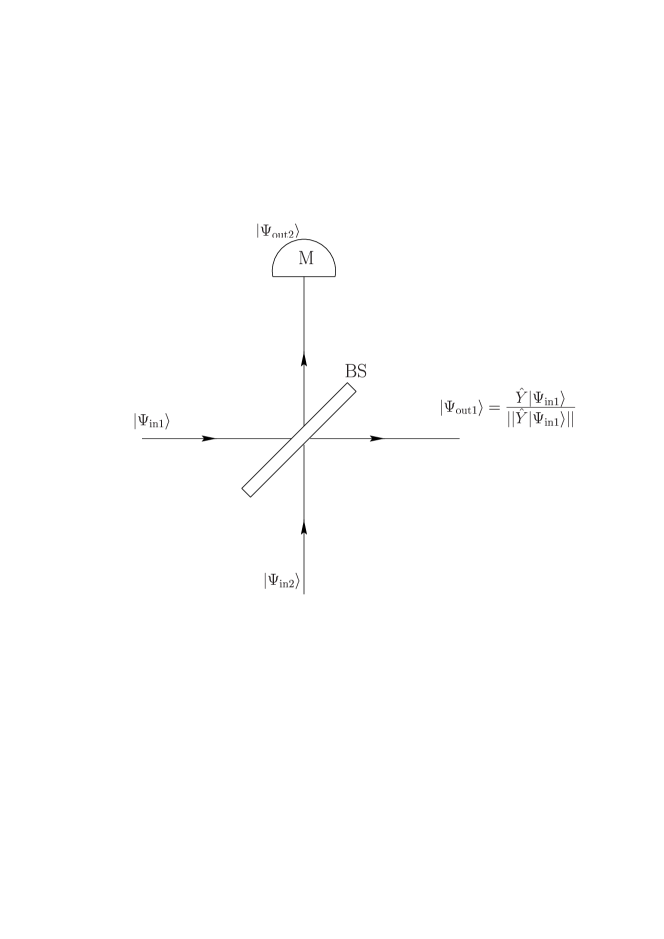
Figure 1: After mixing a signal mode prepared in the state $|\Psi_{{\rm in}_{1}}\rangle$ with a reference mode prepared in the state $|\Psi_{{\rm in}_{2}}\rangle$, the output signal mode collapses to the state $|\Psi_{{\rm out}_{1}}\rangle$, if the measuring instrument M projects the output reference mode onto the state $|\Psi_{{\rm out}_{2}}\rangle$.

Let us consider an experimental setup of the type shown in figure 1. A signal mode (index 1) is mixed with a reference mode (index 2) at a beam splitter, and a measurement (device M) is performed on the output reference mode. Since the two output modes are entangled in general, the measurement influences the output signal mode as well. The action of a beam splitter can be described by a unitary operator $\hat{U}$ connecting the input and output states according to

$$|\Psi_{{\rm out}}\rangle=\hat{U}|\Psi_{{\rm in}}\rangle\,,$$ (1)

where [12]

$$\hat{U}=e^{\i(\varphi_{T}+\varphi_{R})\hat{L}_{3}}e^{2i\vartheta\hat{L}_{2}}e^{\i(\varphi_{T}-\varphi_{R})\hat{L}_{3}},$$ (2)

with

$$\hat{L}_{2}=\frac{1}{2\i}(\hat{a}_{1}^{\dagger}\hat{a}_{2}-\hat{a}_{2}^{+}\hat{a}_{1}),\qquad\hat{L}_{3}=\frac{1}{2}(\hat{a}_{1}^{\dagger}\hat{a}_{1}-\hat{a}_{2}^{\dagger}\hat{a}_{2})\,,$$ (3)

and the complex transmittance $T$ and reflectance $R$ of the beam splitter are defined by

$$T=e^{\i\varphi_{T}}\cos\vartheta,\qquad R=e^{\i\varphi_{R}}\sin\vartheta.$$ (4)

Now let us assume that $\hat{\Pi}(l)$ is the positive operator valued measure (POVM) that is realized by the measuring device M, with

$$\hat{\Pi}(l)\geq 0,\qquad\sum_{l}\hat{\Pi}(l)=1$$ (5)

(for POVM, see, e.g., [15, 16]). When the measurement on the output reference mode yields the result $l$, then the reduced state of the output signal mode becomes

$$\hat{\varrho}_{{\rm out}_{1}}=\frac{{\rm Tr}_{2}\!\left[\hat{\varrho}_{{\rm out}}\hat{\Pi}(l)\right]}{p(l)}\,,\qquad\hat{\varrho}_{{\rm out}}=\hat{U}|\Psi_{{\rm in}}\rangle\langle\Psi_{{\rm in}}|\hat{U}^{\dagger},$$ (6)

where

$$p(l)=\langle\hat{\Pi}(l)\rangle={\rm Tr}_{1}{\rm Tr}_{2}\!\left[\hat{\varrho}_{{\rm out}}\hat{\Pi}(l)\right]$$ (7)

is the probability of obtaining the result $l$. In particular, when $\hat{\Pi}(l)$ projects onto a pure state $|l\rangle$ $\!=$ $\!|\Psi_{{\rm out}_{2}}\rangle$, i.e.,

$$\hat{\Pi}(l)=|\Psi_{{\rm out}_{2}}\rangle\langle\Psi_{{\rm out}_{2}}|,$$ (8)

and the (pure) input state can be decomposed as

$$|\Psi_{{\rm in}}\rangle=|\Psi_{{\rm in}_{1}}\rangle|\Psi_{{\rm in}_{2}}\rangle,$$ (9)

then combination of equations (6) – (9) yields

$$\hat{\varrho}_{{\rm out}_{1}}=|\Psi_{{\rm out}_{1}}\rangle\langle\Psi_{{\rm out}_{1}}|,$$ (10)

with

$$|\Psi_{{\rm out}_{1}}\rangle=\frac{\hat{Y}|\Psi_{{\rm in}_{1}}\rangle}{\|\hat{Y}|\Psi_{{\rm in}_{1}}\rangle\|}\,,$$ (11)

where

$$\hat{Y}=\langle\Psi_{{\rm out}_{2}}|\hat{U}|\Psi_{{\rm in}_{2}}\rangle,$$ (12)

is the non-unitary conditional beam splitter operator $\hat{Y}$ defined in the signal-mode Hilbert space, the expectation value of $\hat{Y}^{\dagger}\hat{Y}$ being the probability of obtaining the state $|\Psi_{{\rm out}_{1}}\rangle$,

$$p(\Psi_{{\rm out}_{1}})=\|\hat{Y}|\Psi_{{\rm in}_{1}}\rangle\|^{2}\equiv\langle\Psi_{{\rm in}_{1}}|\hat{Y}^{\dagger}\hat{Y}|\Psi_{{\rm in}_{1}}\rangle.$$ (13)

In order to determine the non-unitary transformation operator $\hat{Y}$, let us first consider reference modes that are prepared in displaced Fock states (for displaced Fock states, see, e.g., [17] and references therein),

$$|\Psi_{{\rm in}_{2}}\rangle=\hat{D}_{2}(\alpha)|m\rangle_{2}\,,\qquad|\Psi_{{\rm out}_{2}}\rangle = \hat{D}_{2}(\beta)|n\rangle_{2}\,,$$ (14)

with $\hat{D}(\alpha)$ $\!=$ $\!{\rm exp}(\alpha\hat{a}^{\dagger}$ $\!-$ $\!\alpha^{*}\hat{a})$ being the coherent displacement operator. After a lengthy but straightforward calculation (see Appendix A) we find that

$$\hat{Y}=\hat{D}_{1}\!\left(\frac{\alpha-T\beta}{R^{\ast}}\right)\,_{2}\langle n|\hat{U}|m\rangle_{2}\,\hat{D}_{1}\!\left(\frac{\beta-T^{*}\alpha}{R^{*}}\right),$$ (15)

where

$${}_{2}\langle n|\hat{U}|m\rangle_{2}=\frac{R^{m}(-R^{*})^{n}}{T^{n}\sqrt{m!n!}}\left\{(\hat{a}_{1}^{\dagger})^{m}\hat{a}_{1}^{n}\right\}_{s}T^{\hat{n}_{1}}.$$ (16)

Here, the notation $\{\cdots\}_{s}$ introduces $s$-ordering (for $s$-ordering, see [18]), with

$$s=\frac{2}{|R|^{2}}-1.$$ (17)

Note that $s$ $\!>$ $\!1$. Applying equation (A12) for $t$ $\!=$ $\!1$ and using the formulas given in Appendix A in Ref. [6], the $s$-ordered operator product in equation (16) can be rewritten as

$$\{(\hat{a}^{\dagger})^{m}\hat{a}^{n}\}_{s}\!=\!\left\{\begin{array}[]{c@{\quad{\rm if}\quad}l}\displaystyle m!\left[-\frac{s\!+\!1}{2}\right]^{m}\hat{a}^{n-m}\,{\rm P}_{m}^{(n-m,\hat{n}-n)}\!\left[\frac{s\!-\!3}{s\!+\!1}\right]&m\leq n,\\[10.76385pt] \displaystyle n!\left[-\frac{s\!+\!1}{2}\right]^{n}(\hat{a}^{\dagger})^{m-n}\,{\rm P}_{n}^{(m-n,\hat{n}-n)}\!\left[\frac{s\!-\!3}{s\!+\!1}\right]&m\geq n,\end{array}\right.$$ (20)

where ${\rm P}_{a}^{(b,c)}(z)$ is the Jacobi polynomial. It should be mentioned that when $\alpha$ $\!=$ $\!\beta$ $\!=$ $\!0$, then the operator $\hat{Y}$ in equation (15) realizes the transformation to the Jacobi-Polynomial states in Ref. [6].

Now, the generalization of the formalism to arbitrary (pure) quantum states of the reference modes,

$$|\Psi_{{\rm in}_{2}}\rangle=\hat{F}(\hat{a}_{2}^{\dagger})|0\rangle_{2}\,,\qquad|\Psi_{{\rm out}_{2}}\rangle=\hat{G}(\hat{a}_{2}^{\dagger})|0\rangle_{2}\,,$$ (21)

is straightforward. From equations (12) and (21) and application of the relation (16) $\hat{Y}$ is obtained to be

$$\hat{Y}=\left\{\hat{F}(R\hat{a}_{1}^{\dagger})\,\hat{G}^{\dagger}\!\left(-\frac{R}{T^{*}}\hat{a}_{1}^{\dagger}\right)\right\}_{s}T^{\hat{n}_{1}}.$$ (22)

The result reveals, that (up to the operator $T^{\hat{n}_{1}}$) the non-unitary conditional beam splitter operator $\hat{Y}$ is nothing but the operator product $\hat{F}\hat{G}^{\dagger}$ in $s$ order, with $s$ from equation (17). Although equation (22) already covers the general case, it may be useful, for practical reasons, to consider explicitly coherently displaced quantum states of the reference modes, that is

$$|\Psi_{{\rm in}_{2}}\rangle=\hat{D}_{2}(\alpha)\hat{F}(\hat{a}_{2}^{\dagger})|0\rangle_{2}\,,\qquad|\Psi_{{\rm out}_{2}}\rangle=\hat{D}_{2}(\beta)\hat{G}(\hat{a}_{2}^{\dagger})|0\rangle_{2}\,.$$ (23)

In close analogy to the derivation of equations (15) and (22) we find that

$$\hat{Y}=\hat{D}_{1}\!\left(\frac{\alpha-T\beta}{R^{*}}\right)\,\left\{\hat{F}(R\hat{a}_{1}^{\dagger})\,\hat{G}^{\dagger}\!\left(-\frac{R}{T^{*}}\hat{a}_{1}^{\dagger}\right)\right\}_{s}T^{\hat{n}_{1}}\,\hat{D}_{1}\!\left(\frac{\beta-T^{*}\alpha}{R^{*}}\right),$$ (24)

which shows that displacing the quantum states of the reference modes always leads to displaced quantum states of the signal modes.

From equation (24) it is easily seen that the ordering procedure can be omitted if at least one of the reference modes is prepared in a coherent state (the vacuum included), i.e., $\hat{F}$ $\!=$ $\!\hat{I}$ or $\hat{G}$ $\!=$ $\!\hat{I}$. This is the case when, e.g., $|\Psi_{{\rm in}_{2}}\rangle$ $\!=$ $\!|0\rangle_{2}$ and $|\Psi_{{\rm out}_{2}}\rangle$ $\!=$ $\!|n\rangle_{2}$ (or $|\Psi_{{\rm in}_{2}}\rangle$ $\!=$ $\!|n\rangle_{2}$ and $|\Psi_{{\rm out}_{2}}\rangle$ $\!=$ $\!|0\rangle_{2}$), which leads to preparation of the output signal mode in a photon-subtracted (or photon-added) state [4, 5]. Note that preparation of the output reference mode in a coherent state can be realized in eight-port homodyne detection or heterodyne detection. Further it should be mentioned that $|\Psi_{{\rm in}_{1}}\rangle$ and $|\Psi_{{\rm in}_{2}}\rangle$ can be interchanged if $T$ and $R$ are replaced with i$R$ and i$T$, respectively, because of the symmetry of the beam splitter transformation [12]. The operator $\hat{Y}$ then transforms (up to a global phase factor) the state $|\Psi_{{\rm in}_{2}}\rangle$ into the state $|\Psi_{{\rm out}_{1}}\rangle$. In this way the $s$-ordering procedure can also be circumvented when the signal mode is prepared in a coherent state.

In general, the POVM realized by the measurement apparatus does not project onto a pure state, and equation (8) must be replaced with

$$\hat{\Pi}(l)=\sum_{\Psi_{{\rm out}_{2}}}p(l|\Psi_{{\rm out}_{2}})|\Psi_{{\rm out}_{2}}\rangle\langle\Psi_{{\rm out}_{2}}|\,,$$ (25)

where $p(l|\Psi_{{\rm out}_{2}})$ is the probability of obtaining the measurement outcome $l$ under the condition that the output reference mode is prepared in the state $|\Psi_{{\rm out}_{2}}\rangle$. A typical example is direct photon counting with quantum efficiency $\eta$ less than unity,

$$\hat{\Pi}(n)=\sum_{k}{k\choose n}\eta^{n}(1-\eta)^{k-n}|k\rangle_{2\,\,2}\langle k|\,.$$ (26)

Further, the input reference mode may also be prepared in a mixed quantum state,

$$\hat{\varrho}_{{\rm in}_{2}}=\sum_{\Psi_{{\rm in}_{2}}}p(\Psi_{{\rm in}_{2}})|\Psi_{{\rm in}_{2}}\rangle\langle\Psi_{{\rm in}_{2}}|\,,$$ (27)

so that for an input quantum state

$$\hat{\varrho}_{{\rm in}}=\hat{\varrho}_{{\rm in}_{1}}\otimes\hat{\varrho}_{{\rm in}_{2}}$$ (28)

the quantum state of the output signal mode now reads

$$\hat{\varrho}_{{\rm out}_{1}}=\frac{1}{p(l)}\sum_{\Psi_{{\rm in}_{2}}}p(\Psi_{{\rm in}_{2}})\sum_{\Psi_{{\rm out}_{2}}}p(l|\Psi_{{\rm out}_{2}})\hat{Y}\hat{\varrho}_{{\rm in}_{1}}\hat{Y}^{\dagger}$$ (29)

in place of (11), where $\hat{Y}$ is defined by equation (12). In equation (29)

$$p(l)=\sum_{\Psi_{{\rm in}_{2}}}p(\Psi_{{\rm in}_{2}})\sum_{\Psi_{{\rm out}_{2}}}p(l|\Psi_{{\rm out}_{2}}){\rm Tr}_{1}\!\left(\hat{Y}\hat{\varrho}_{{\rm in}_{1}}\hat{Y}^{\dagger}\right).$$ (30)

is the probability of obtaining the measurement outcome $l$, i.e., the probability of producing the output signal-mode quantum state $\hat{\varrho}_{{\rm out}_{1}}$.

3 Creation of Schrödinger-cat-like states

In order to illustrate the theory, let us consider the generation of Schrödinger-cat-like states. A possible way is to prepare the input signal mode in a squeezed vacuum, combine it with an input reference mode prepared in a Fock state (including the vacuum state) and perform a photon-number measurement on the output reference mode [4, 5]. Here we present two alternative schemes that are only based on Fock states and coherent states. Let us first consider a scheme [figure 2(a)] that uses a Fock state source and displaced photon-number measurement,

$$|\Psi_{{\rm in}_{1}}\rangle=|n\rangle,$$ (31)

$$|\Psi_{{\rm in}_{2}}\rangle=|0\rangle,\qquad|\Psi_{{\rm out}_{2}}\rangle=\hat{D}(\beta^{\prime})|n\rangle.$$ (32)

For notational convenience we omit the subscripts $1$ and $2$ introduced in Section 2 in order to distinguish between the channels. Application of equations (11) and (15) then yields ($|T|^{2}$ $\!=$ $\!0.5$)

$$|\Psi_{{\rm out}_{1}}\rangle=:|\chi_{n}^{n,\beta}\rangle = \frac{1}{n!\sqrt{N}}\big{(}\hat{a}-\beta\big{)}^{n}\big{(}\hat{a}^{\dagger}+\beta^{*}\big{)}^{n}|0\rangle$$ (33)

$$= N^{-1/2}\sum_{k=0}^{n}{\rm L}_{n-k}^{k}\!\left(|\beta|^{2}\right)\,\frac{(-\beta\hat{a}^{\dagger})^{k}}{k!}\,|0\rangle$$

$$= N^{-1/2}{\rm L}_{n}\!\left[\beta\hat{D}^{\dagger}(\beta)\hat{a}^{\dagger}\hat{D}(\beta)\right]|0\rangle$$

[$\beta$ $\!=$ $\!\beta^{\prime}e^{\i(\varphi_{T}+\varphi_{R}+\pi)}$; ${\rm L}_{n}(z)$, Laguerre polynomial; ${\rm L}_{n}^{a}(z)$, associated Laguerre polynomial], where

$$2^{-n}e^{-|\beta|^{2}}\,N=2^{-n}e^{-|\beta|^{2}}\sum_{k=0}^{n}\frac{|\beta|^{2k}}{k!}\,{\rm L}_{n-k}^{k}\!\left(|\beta|^{2}\right)^{2}=p(n,\beta^{\prime}),$$ (34)

$p(n,\beta^{\prime})$ being the probability of generating the state $|\chi_{n}^{n,\beta}\rangle$ for given $\beta^{\prime}$ [see equation (13)]. Equation (33) reveals that the quantum state of output signal mode is obtained by applying an operator Laguerre polynomial ${\rm L}_{n}$ on the vacuum state. As it is seen from the in figure 3 plotted contours of the Husimi function

$$Q(\alpha)=\frac{1}{\pi}|\langle\alpha|\chi_{n}^{n,\beta}\rangle|^{2}=\frac{1}{\pi N}\left|{\rm L}_{n}[\beta(\alpha^{\ast}\!+\!\beta^{\ast}]\right|^{2}e^{-|\alpha|^{2}},$$ (35)

the state $|\chi_{n}^{n,\beta}\rangle$ exhibits for $|\beta|^{2}$ $\!=$ $\!n/2$ two well separated peaks in the phase space, which are approximately located at $\pm{\rm i}\beta$ [figure 3(b)]. It should be noted that the distance of the peaks increases with the square root of the detected photons, which is analogous to the behaviour of the Schrödinger-cat-like states considered in [4]. The Husimi $Q$ function, which can be directly measured, e.g., in eight-port homodyne detection or heterodyne detection, is a rather smeared phase-space function, because of the included vacuum noise. More details of the structure of the state can be inferred from the Wigner function

$$W(x,p)=\frac{1}{\pi}\int_{-\infty}^{+\infty}dy\,{\rm e}^{2{\rm i}py}\langle x-y,0|\chi_{n}^{n,\beta}\rangle\langle\chi_{n}^{n,\beta}|x+y,0\rangle,$$ (36)

where $|x,0\rangle$ is the quadrature-component state

$$|x,\varphi\rangle=(\pi)^{-\frac{1}{4}}\exp\!\left(-\textstyle\frac{1}{2}x^{2}\right)\sum_{k=0}^{\infty}\frac{e^{\i k\varphi}}{\sqrt{2^{k}k!}}\,{\rm H}_{k}(x)|k\rangle$$ (37)

for $\varphi$ $\!=$ $\!0$ [H${}_{k}(z)$, Hermite polynomial]. Using equations (33) and (37) and applying standard formulas [19], the $y$-integral in equation (36) can be calculated to obtain

$$W(x,p)=\frac{e^{-(x^{2}+p^{2})}}{\pi N}\sum_{m=0}^{n}\Bigg{\{}\sum_{k=0}^{m}{\rm L}_{n-k}^{k}\big{(}|\beta|^{2}\big{)}{\rm L}_{n-m}^{m}\big{(}|\beta|^{2}\big{)}{\rm L}_{k}^{m-k}\big{(}|z|^{2}\big{)}\beta^{k}\big{(}-\beta^{\ast}\big{)}^{m}\frac{z^{m-k}}{m!}$$ (38)

$$+\!\!\sum_{k=m+1}^{n}\!\!{\rm L}_{n-k}^{k}\big{(}|\beta|^{2}\big{)}{\rm L}_{n-m}^{m}\big{(}|\beta|^{2}\big{)}{\rm L}_{k}^{k-m}\big{(}|z|^{2}\big{)}\beta^{k}\big{(}-\beta^{\ast}\big{)}^{m}\frac{(-z^{\ast})^{k-m}}{k!}\Bigg{\}}$$

[$z\!=\!\sqrt{2}(x$ $\!+$ $\!ip)$]. The Wigner function is a measurable quantity which however does not correspond to a POVM. Let us therefore also consider the quadrature-component probability distributions

$$p(x,\varphi) = |\langle x,\varphi|\chi_{n}^{n,\beta}\rangle|^{2}$$ (39)

$$= \frac{1}{\pi^{\frac{1}{2}}N}\left|\sum_{k=0}^{n}{\rm L}_{n-k}^{k}(|\beta|^{2})\frac{(-2^{-\frac{1}{2}}\beta^{\ast}e^{\i\varphi})^{k}}{k!}{\rm H}_{k}(x)\right|^{2}e^{-x^{2}},$$

which also contain all available information on the quantum state and can be directly measured in four-port homodyne detection. Plots of the Wigner function and the quadrature-component distributions of the state $|\chi_{n}^{n,\beta}\rangle$ for $\beta$ $\!=$ $\!\sqrt{n/2}$ are presented in figures 4 and 5 respectively. They clearly reveal the typical features of Schrödinger-cat-like states. The probability of producing the state for various values of $n$ is shown in figure 6.

Let us compare the scheme in figure 2(a) with the somewhat modified scheme in figure 2(b). In the latter scheme the input signal mode that is prepared in a coherent state is mixed with an input reference mode that is prepared in a Fock state, and a photon-number measurement is performed on the output reference mode,

$$|\Psi_{{\rm in}_{1}}\rangle = |\beta/T\rangle,$$ (40)

$$|\Psi_{{\rm in}_{2}}\rangle=|n\rangle,\qquad|\Psi_{{\rm out}_{2}}\rangle=|n\rangle.$$ (41)

The scheme realizes the generation of a special Jacobi-polynomial coherent state [6],

$$|\Psi_{{\rm out}_{1}}\rangle \sim \{(\hat{a}^{+})^{n}\hat{a}^{n}\}_{s=3}\,T^{\hat{n}}\,|\beta/T\rangle\,\sim\,{\rm P}_{n}^{(0,\hat{n}-n)}(0)\,|\beta\rangle$$ (42)

$$\sim {\rm L}_{n}\!\left(\beta\hat{a}^{\dagger}\right)|\beta\rangle\,=\,\hat{D}(\beta)\,|\chi_{n}^{n,\beta}\rangle$$

($|T|^{2}$ $\!=$ $\!0.5$). Here we have used equations (15), (16) and (20) and the relation ${\hat{n}\choose k}$ $\!=$ $\!(\hat{a}^{\dagger})^{k}\hat{a}^{k}/k!$. Comparing equations (33) and (42), we see that the states produced in the schemes in figures 2(a) and 2(b) differ in a coherent displacement. Obviously, the coherently displaced state shows again for $|\beta|^{2}$ $\!=$ $\!n/2$ the typical features of a Schrödinger-cat-like state, the phase difference between the component states being $\pi/2$. The probability of producing the state is the same as in equation (34).

It is worth noting that replacing in equation (33) $(\hat{a}$ $\!-$ $\!\beta)$ with $(\hat{a}$ $\!-$ $\!\beta)^{\dagger}$ yields the state

$$|\psi_{n,\beta}^{(2)}\rangle=\frac{1}{\sqrt{N_{2}}}\left(\hat{a}^{\dagger}\!-\!\beta^{*}\right)^{n}\left(\hat{a}^{\dagger}\!+\!\beta^{*}\right)^{n}|0\rangle=\frac{1}{\sqrt{N_{2}}}\left[\left(\hat{a}^{\dagger}\right)^{2}\!-\!\left(\beta^{*}\right)^{2}\right]^{n}|0\rangle,$$ (43)

the properties of which are similar to those of the state $|\chi_{n}^{n,\beta}\rangle$ in equation (33). States of the type (43) may be produced, e.g., by two displaced $n$-photon-additions (for such schemes, see [11]). The generalization to $k$ displaced $n$-photon-additions is straightforward,

$$|\psi_{n,\beta}^{(k)}\rangle=\frac{1}{\sqrt{N_{k}}}\left[\left(\hat{a}^{\dagger}\right)^{k}-\left(\beta^{*}\right)^{k}\right]^{n}|0\rangle,$$ (44)

$$N_{k}=\sum_{j=0}^{n}{n\choose j}^{2}|\beta|^{2k(n-j)}(kj)!.$$ (45)

States of this type can be regarded, for appropriately chosen $\beta$, as multiple Schrödinger-cat-like states [21], as it can be seen from figure 7, in which the Husimi function

$$Q(\alpha)=\frac{1}{\pi N_{k}}\left|\alpha^{k}-\beta^{k}\right|^{2n}e^{-|\alpha|^{2}}$$ (46)

of such a state is plotted.

4 Conclusions

In this paper we have studied conditional quantum-state generation at a beam splitter, regarding the apparatus as an effective two-port device, which is described by a non-unitary beam splitter operator $\hat{Y}$ that acts in the Hilbert space of the signal mode only. We have presented the $\hat{Y}$ operator for arbitrary quantum states $|\Psi_{{\rm in}_{2}}\rangle$ and $|\Psi_{{\rm out}_{2}}\rangle$ of the reference mode as an $s$-ordered operator product of those operators which generate $|\Psi_{{\rm in}_{2}}\rangle$ and $\langle\Psi_{{\rm out}_{2}}|$ from the vacuum, $s$ being entirely determined by the absolute value of the reflectance (or transmittance) of the beam splitter. We have further given a generalization to the case of mixed input states and non-perfect measurement.

The formalism is a generalization of previously obtained results, which are easily recovered by appropriate specification of the non-unitary transformation operator. Given the quantum state of the input signal, the conditional quantum state of the output signal can be calculated in a very straightforward way for arbitrary input reference states and arbitrary measurement-assistant projection. The probability of producing the conditional quantum state of the output signal is simply given by its norm. In order to illustrate the theory, we have considered two schemes for generating Schrödinger-cat-like states and addressed the problem of generating multiple Schrödinger-cat-like states. Finally, it should be pointed out that the formalism developed is also suitable for studying state manipulation and state engineering via conditional measurement at multiports that are built up by beam splitters, such as chains of beam splitters.

Appendix Appendix A Derivation of Equation (15)

From equations (12) and (14) the operator $\hat{Y}$ is defined by

$$\hat{Y}=\,_{2}\langle n|\hat{D}_{2}^{\dagger}(\beta)\hat{U}\hat{D}_{2}(\alpha)|m\rangle_{2}\,,$$ (A1)

where $\hat{U}$, equation (2), can be rewritten as [5]

$$\hat{U}=e^{\i(\varphi_{T}\!+\!\varphi_{R})\hat{L}_{3}}e^{2\i\vartheta\hat{L}_{2}}e^{\i(\varphi_{T}-\varphi_{R})\hat{L}_{3}}=T^{\hat{n}_{1}}e^{-R^{\ast}\hat{a}^{\dagger}_{2}\hat{a}_{1}}e^{R\hat{a}^{\dagger}_{1}\hat{a}_{2}}T^{-\hat{n}_{2}}\,.$$ (A2)

We insert equation (A2) into equation (A1) and calculate the channel-2 matrix element as

$$\hat{Y}=\frac{1}{\sqrt{m!n!}}\;_{2}\langle\beta|(\hat{a}_{2}-\beta)^{n}T^{\hat{n}_{1}}e^{-R^{\ast}\hat{a}^{\dagger}_{2}\hat{a}_{1}}e^{R\hat{a}^{\dagger}_{1}\hat{a}_{2}}T^{-\hat{n}_{2}}(\hat{a}_{2}^{\dagger}-\alpha^{\ast})^{m}|\alpha\rangle_{2},$$ (A3)

where we have used the relation

$$\hat{D}^{-1}(\alpha)f(\hat{a},\hat{a}^{\dagger})\hat{D}(\alpha)=f(\hat{a}\!+\!\alpha,\hat{a}^{\dagger}\!+\!\alpha^{\ast})$$ (A4)

and $|n\rangle\!=\!1/\sqrt{n!}(\hat{a}^{\dagger})^{n}|0\rangle$. Applying the relations

$$e^{\varphi\hat{n}}f(\hat{a})=f(e^{-\varphi}\hat{a})e^{\varphi\hat{n}},\qquad e^{\varphi\hat{n}}f(\hat{a}^{\dagger})=f(e^{\varphi}\hat{a}^{\dagger})e^{\varphi\hat{n}},$$

$$e^{\varphi\hat{a}^{\dagger}}f(\hat{a})=f(\hat{a}\!-\!\varphi)e^{\varphi\hat{a}^{\dagger}},\qquad e^{\varphi\hat{a}}f(\hat{a}^{\dagger})=f(\hat{a}^{\dagger}\!+\!\varphi)e^{\varphi\hat{a}},$$ (A5)

after straightforward algebra we derive

$$\hat{Y}=\frac{T^{\hat{n}_{1}}e^{-R^{\ast}\beta^{\ast}\hat{a}_{1}}}{\sqrt{m!n!}}\sum_{k=0}^{m}\sum_{l=0}^{n}{m\choose k}{n\choose l}T^{-k}\left(-\beta\!-\!R^{\ast}\hat{a}_{1}\right)^{n-l}$$ (A6)

$$\hskip 43.05542pt\times\;\left[-\alpha^{\ast}\!+\!\frac{R}{T}\,\hat{a}_{1}^{+}\right]^{m-k}\!_{2}\langle\beta|\hat{a}_{2}^{l}(\hat{a}_{2}^{\dagger})^{k}T^{-\hat{n}_{2}}|\alpha\rangle_{2}\,e^{(R/T)\alpha\hat{a}^{\dagger}_{1}}.$$

Using the ordering formula [18]

$$\hat{a}^{m}(\hat{a}^{\dagger})^{n}=\sum_{l=0}^{\min\{m,n\}}{m\choose l}\frac{n!}{(n-l)!}(\hat{a}^{\dagger})^{n-l}\hat{a}^{m-l}$$ (A7)

together with equation (A5) and the relation

$$T^{\hat{n}}|\alpha\rangle=e^{-|\alpha|^{2}(1-|T|^{2})/2}|T\alpha\rangle,$$ (A8)

we have

$$\hat{Y}=\frac{T^{\hat{n}_{1}}}{\sqrt{m!n!}}\,e^{\alpha\beta^{\ast}/T}e^{-(|\alpha|^{2}+|\beta|^{2})/2}\sum_{k=0}^{m}\sum_{l=0}^{n}\sum_{j=0}^{\min\{k,l\}}{m\choose k}{n\choose l}j!{k\choose j}{l\choose j}(\beta^{*})^{k-j}$$ (A9)

$$\times\alpha^{l-j}\,T^{j-k-l}\,e^{-R^{*}\beta^{*}\hat{a}_{1}}\left(-\beta\!-\!R^{\ast}\hat{a}_{1}\right)^{n-l}\left(-\alpha^{\ast}\!+\!\frac{R}{T}\,\hat{a}_{1}^{\dagger}\right)^{m-k}e^{(R/T)\alpha\hat{a}^{\dagger}_{1}}.$$

Changing the summation indices, some of the finite summations may be performed to obtain

$$\hat{Y}=\frac{T^{\hat{n}_{1}-m}}{\sqrt{m!n!}}\,e^{\alpha\beta^{\ast}/T}e^{-(|\alpha|^{2}+|\beta|^{2})/2}\sum_{k=0}^{\min\{m,n\}}{m\choose k}{n\choose k}k!$$ (A10)

$$\times\,e^{-R^{*}\beta^{*}\hat{a}_{1}}\left(-R^{*}\hat{a}_{1}\!+\!\frac{\alpha}{T}\!-\!\beta\right)^{n-k}\left(R\hat{a}_{1}^{\dagger}\!-\!T\alpha^{\ast}\!+\!\beta^{\ast}\right)^{m-k}e^{(R/T)\alpha\hat{a}^{\dagger}_{1}}.$$

Applying again the relations (A4) and (A5), after some calculation we obtain

$$\hat{Y}=\frac{T^{-m}}{\sqrt{m!n!}}\,\hat{D}_{1}\!\left(\frac{\alpha\!-\!T\beta}{R^{*}}\right)\Bigg{\{}\sum_{k=0}^{\min\{m,n\}}k!{m\choose k}{n\choose k}\left[\frac{-1\!-\!(2|R|^{-2}-1)}{2}\right]^{k}$$ (A11)

$$\times\,(-|R|^{2})^{k}\left(-\frac{R^{*}}{T}\right)^{n-k}(RT)^{m-k}\hat{a}_{1}^{n-k}(\hat{a}_{1}^{\dagger})^{m-k}T^{\hat{n}_{1}}\Bigg{\}}\hat{D}_{1}\!\left(\frac{\beta\!-\!T^{\ast}\alpha}{R^{\ast}}\right).$$

Making use of the standard ordering formula [18]

$$\left\{(\hat{a}^{\dagger})^{m}\hat{a}^{n}\right\}_{s}=\sum_{k=0}^{\min\{m,n\}}k!{m\choose k}{n\choose k}\left(\frac{t-s}{2}\right)^{k}\left\{(\hat{a}^{\dagger})^{m-k}\hat{a}^{n-k}\right\}_{t}$$ (A12)

for $t$ $\!=$ $\!-1$, we eventually arrive at equation (15) (for more details, see [22]).

References

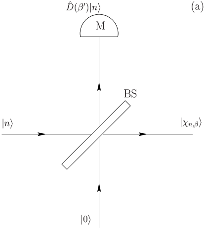
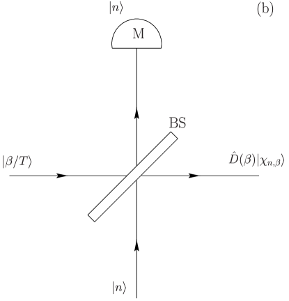
Figure 2: (a) A Fock state $|n\rangle$ is fed into a balanced beam splitter. When the measuring instrument M projects the output reference mode onto a displaced Fock state $\hat{D}(\beta^{\prime})|n\rangle$, then for $|\beta^{\prime}|^{2}$ $\!=$ $\!|\beta|^{2}$ $\!=$ $\!n/2$ the output signal mode collapses to the Schrödinger-cat-like state $|\chi_{n}^{n,\beta}\rangle$, equation (33).
(b) A coherent state $|\beta/T\rangle$ and a Fock state $|n\rangle$ are fed into a balanced beam splitter. When the measuring instrument M projects the output reference mode onto the same Fock state $|n\rangle$, then the output signal mode collapses to the state $\hat{D}(\beta)|\chi_{n}^{n,\beta}\rangle$.

Figure 3: Contour plots of the Husimi function $Q(\alpha)$, equation (35), of the state $|\chi_{n}^{n,\beta}\rangle$, equation (33), for $n$ $\!=$ $\!10$ and (a) $\beta$ $\!=$ $\!\sqrt{n/10}$, (b) $\beta$ $\!=$ $\!\sqrt{n/2}$, and (c) $\beta$ $\!=$ $\!\sqrt{2.5n}$.

Figure 4: The Wigner function $W(x,p)$, equation (38), of the state $|\chi_{n}^{n,\beta}\rangle$, equation (33), is shown for $n$ $\!=$ $\!10$ and $\beta$ $\!=$ $\!\sqrt{n/2}$.

Figure 5: The quadrature-component probability distributions $p(x,\varphi)$, equation (39), of the state $|\chi_{n}^{n,\beta}\rangle$, equation (33), are shown for $n=10$ and $\beta=\sqrt{n/2}$.

Figure 6: The probability $p(n,\beta^{\prime})$, equation (34), of producing the state $|\chi_{n}^{n,\beta}\rangle$, equation (33), is shown as a function of $n$ for $|\beta^{\prime}|^{2}$ $\!=$ $\!|\beta|^{2}$ $\!=n/2$.

Figure 7: The Husimi function $Q(\alpha)$, equation(46), of the state $|\psi_{n,\beta}^{(k)}\rangle$, equation (44), is shown for $n$ $\!=$ $\!10$, $k$ $\!=$ $\!5$, and $\beta$ $\!=$ $\!4.2$.

References

• [1] Schlienz J and Mahler G 1995 Phys. Rev. A 52 4396
• [2] Steane A 1998 Rep. Prog. Phys. 61 117
• [3] Ban M 1996 J. Mod. Opt. 43 1281
• [4] Dakna M, Anhut T, Opatrný T, Knöll L and Welsch D G 1997 Phys. Rev. A 55 3184
• [5] Dakna M, Knöll L and Welsch D G 1998 Opt. Commun. 145 309
• [6] Dakna M, Knöll L and Welsch D G 1998 Euro. Phys. J. D 3 295
• [7] Ban M 1994 Phys. Rev. A 49 5078
• [8] Ban M 1997 Opt. Commun. 143 225
• [9] Barnett S M and Pegg D T 1996 Phys. Rev. Lett 76 4148
• [10] Pegg D T, Barnett S M and Phillips L S 1997 J. Mod. Opt. 44 2135
• [11] Dakna M, Clausen J, Knöll L and Welsch D G 1998 Phys. Rev. A, in press
• [12] Campos R A, Saleh B E A and Teich M C 1989 Phys. Rev. A 40 1371
• [13] Bužek V and Knight P L, 1995 Progress in Optics XXXIV Edited by Wolf E (North-Holland, Amsterdam)
• [14] Cochrane P T, Milburn G J and Munro W J 1998 [Los Alamos e-print archive quant-ph/9809037]
• [15] Helstrom C W 1976 Quantum Detection and Estimation Theory (New York:Academic Press)
• [16] Busch P, Grabowski M, and Lahti P J 1995 Lecture Notes in Physics m31 Operational Quantum Physics (Berlin Heidelberg New York: Springer)
• [17] Nieto M M 1997 Phys. Lett A 229 135
• [18] Cahill K E and Glauber R J 1969 Phys. Rev. 177 1857
• [19] Prudnikov A P, Brychkov Yu A, and Marichev O J 1986 Integral and Series, Vol 1 and 2 (Gordon and Breach: New Yok).
• [20] Hong-yi F, Xiong Y, Zhi-hua X 1995 Phys. Lett. A 199 131
• [21] Janszky J, Domokos P and Adam P 1993 Phys. Rev. A 48 2213
• [22] Clausen J, 1998 Diploma thesis (Friedrich-Schiller-Universität, Jena)
Refer to caption