Quantum noise in ideal operational amplifiers

Abstract

We consider a model of quantum measurement built on an ideal operational amplifier operating in the limit of infinite gain, infinite input impedance and null output impedance and with a feddback loop. We evaluate the intensity and voltage noises which have to be added to the classical amplification equations in order to fulfill the requirements of quantum mechanics. We give a description of this measurement device as a quantum network scattering quantum fluctuations from input to output ports.

PACS: 42.50Lc 03.65Bz 07.50Qx

Modern measurement techniques and especially ultrasensitive ones often involve active systems. Such devices may be used either for a preamplification purpose when a microscopic signal is amplified to an observable macroscopic level, or for a stabilization purpose when a feedback loop keeps the system in the vicinity of an optimal working point. Amplifiers thus play a crucial role in ultrasensitive measurements and this should be accounted for in theoretical analysis of ultimate sensitivities attainable in quantum measurements.

Quantum noise associated with linear amplifiers has been the subject of numerous works. In the line of thought initiated by early works on fluctuation-dissipation relations [1, 2] and continued by a quantum analysis of linear response theory [3, 4], active systems have been studied in the optical domain when maser and laser amplifiers were developed [5, 6, 7]. General thermodynamical constraints impose the existence of fluctuations for amplification as well as for dissipation processes. At the limit of a null temperature, these thermal fluctuations reduce to the quantum fluctuations required by Heisenberg inequalities. This added noise determines the ultimate performance of linear amplifiers [8, 9] and plays a key role in the question of optimal information transfer in optical communication systems [10, 11]. The theory of quantum optical processes has led to the parallel development of a treatment of quantum fluctuations which can be named as ‘quantum network theory’ [12, 13]. It has been applied mainly to optical systems [14, 15] but it has also been viewed as a generalized quantum extension of the linear response theory which is of interest for electrical systems as well [16].

Most practical applications of amplifiers in measurements involve ideal operational amplifiers operating near the limits of infinite gain, infinite input impedance and null output impedance. It could appear difficult to deal with these limits without pathologies in the treatment of fluctuations. In the present letter we show how this difficulty may be circumvented.

To this aim, we study a model of quantum measurement performed with an ideal operational amplifier. The model, sketched on Figure 1, consists in an ideal operational amplifier operating with a feedback loop and connecting two coaxial lines denoted $l$ and $r$ for left and right. These two lines will be associated respectively with signal and readout. The presence of a feedback loop fixes the effective gain and effective impedances of the device. It entails that a third line $f$ has to be introduced to account for the fluctuations associated with the dissipative part of the feedback impedance. We show in the letter that the ultimate performances of this measurement device may be characterized in a precise manner. Fluctuations added by the amplifier are described in terms of noise spectra of equivalent voltage and current generators. Since these fluctuations account for quantum as well as thermodynamical constraints, they are described by non commuting operators and obey Heisenberg inequalities.

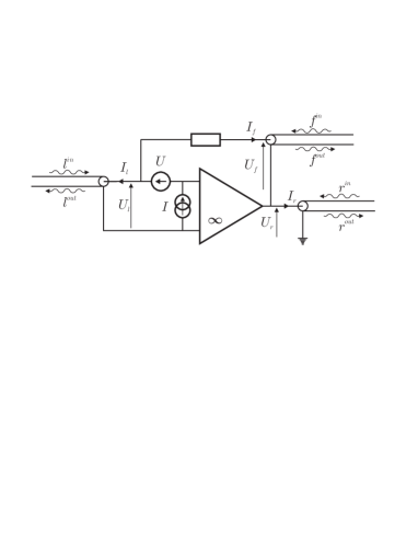
FIG. 1.: Sketch of the quantum measurement apparatus built on an ideal operational amplifier.

Free fields are propagating in the inward and outward directions in each line coupled to the amplifier. The left line comes from a monitored electrical system so that the inward field $l^{\rm in}$ plays the role of the signal to be measured. Meanwhile, the right line goes to an electrical meter so that the outward field $r^{\rm out}$ is the meter readout. In connection with the discussions of Quantum Non Demolition measurements in quantum optical systems [17, 18], $l^{\rm out}$ appears as the back-action field sent back to the monitored system and $r^{\rm in}$ represents the fluctuations coming from the readout line. The feedback loop is partly dissipative and then contains a Nyquist noise source. This Nyquist noise is an extra inward field $f^{\rm in}$ coming through a coaxial line $f$ representing the feedback resistance. The outward field $f^{\rm out}$ represents the way the dissipated energy leaves the system. In principle, information on the measurement can be extracted through this output channel but it is usually lost and the line $f$ is only a noise source in this case.

We now present the electrical equations associated with the measurement device of Fig.1. We first write the characteristic relations between the various voltages and currents

$$U = U_{l}=U_{r}+U_{f}+\left(Z_{f}-R_{f}\right)I_{f}$$ (1)

$$I = I_{l}+I_{f}$$ (2)

Here, $U_{p}$ and $I_{p}$ are the voltage and current at the port $p$, i.e. at the end of the line $p=l$, $r$ or $f$ while $U$ and $I$ are the voltage and current noise generators associated with the operational amplifier itself. $Z_{f}$ is the impedance of the feedback loop and $R_{f}$ its dissipative part, i.e. the characteristic impedance of the line $l$ so that $\left(Z_{f}-R_{f}\right)$ is the reactive impedance of the feedback loop. All equations are implicitly written in the frequency representation and the impedances are functions of frequency. Equations (2) take a simple form because of the limits of infinite gain, infinite input impedance and null output impedance assumed for the operational amplifier. They correspond to the limit of a more general treatment which has been given elsewhere with a finite gain as well as finite input and output impedances [19].

As a second step, we rewrite the voltage and current $U_{p}$ and $I_{p}$ at the port $p$ in terms of the inward and outward fields $p^{\rm in}$ and $p^{\rm out}$ counterpropagating in the line $p$ which has a characteristic impedance $R_{p}$

$$I_{p} = \sqrt{\frac{\hbar\left|\omega\right|}{2R_{p}}}\left(p^{\rm out}-p^{\rm in}\right)$$ (3)

$$U_{p} = \sqrt{\frac{\hbar\left|\omega\right|R_{p}}{2}}\left(p^{\rm out}+p^{\rm in}\right)$$ (4)

The coaxial line being equivalent to a one-dimensional space, the input fields $p^{\rm in}$ may be described by the quantum theory of free fields in a two-dimensional space-time. In particular, they obey the standard commutation relations of such a theory

$$\left[p^{\rm in}\left[\omega\right],p^{\rm in}\left[\omega^{\prime}\right]\right]=2\pi\ \varepsilon\left(\omega\right)\ \delta\left(\omega+\omega^{\prime}\right)$$ (5)

where $\varepsilon\left(\omega\right)$ denotes the sign function. This relation just means that the positive and negative frequency components correspond respectively to the annihilation and creation operators of quantum field theory. Fields corresponding to different lines commute with each other.

The fluctuations of these fields will then be characterized by a noise spectrum $\sigma_{pp}^{\rm in}$ with its well-known expression for a thermal equilibrium at a temperature $T_{p}$

$$\left\langle p^{\rm in}\left[\omega\right]\cdot p^{\rm in}\left[\omega^{\prime}\right]\right\rangle = 2\pi\ \sigma_{pp}^{\rm in}\left[\omega\right]\ \delta\left(\omega+\omega^{\prime}\right)$$ (6)

$$\sigma_{pp}^{\rm in}\left[\omega\right] = \frac{1}{2}\coth\frac{\hbar\left|\omega\right|}{2k_{B}T_{p}}$$ (7)

The dot symbol denotes a symmetrized product and $k_{B}$ is the Boltzmann constant. The quantity $\hbar\left|\omega\right|\sigma_{pp}^{\rm in}$ is the energy per mode. It reduces to the zero point energy $\frac{\hbar\left|\omega\right|}{2}$ at the limit of zero temperature and to the classical result $k_{B}T_{p}$ at the high temperature limit. We also assume that the fields incoming through the various ports are uncorrelated with each other as well as with amplifier noises.

Now the output fields $p^{\rm out}$ have their fluctuations determined by the transformation of the input fields through their interaction with the measurement device. This is the common idea of all input-output descriptions of quantum networks [12, 13, 14, 15, 16, 17]. After this transformation, the field fluctuations are no longer described by the thermal correlation functions given in (7). Moreover, fluctuations are no longer independent in different ports. However the output fields $p^{\rm out}$ still obey the commutation relations (5) of free fields [16]. In the present letter we use this property to characterize the quantum fluctuations of the voltage and current sources associated with the operational amplifier.

To this aim, we use the characteristic equations (2,4) associated with the amplifier and the lines to rewrite the output fields $l^{\rm out}$, $r^{\rm out}$ and $f^{\rm out}$ in terms of input fields $l^{\rm in}$, $r^{\rm in}$, $f^{\rm in}$ and of amplifier noise sources $U$ and $I$

$$l^{\rm out} = -l^{\rm in}+\sqrt{\frac{2}{\hbar\left|\omega\right|R_{l}}}U$$ (8)

$$r^{\rm out} = -r^{\rm in}-2\frac{Z_{f}}{\sqrt{R_{r}R_{l}}}l^{\rm in}-2\sqrt{\frac{R_{f}}{R_{r}}}f^{\rm in}$$ (9)

$$+ \sqrt{\frac{2}{\hbar\left|\omega\right|R_{r}}}\left(\frac{R_{l}+Z_{f}}{R_{l}}U-Z_{f}I\right)$$ (10)

$$f^{\rm out} = f^{\rm in}+2\sqrt{\frac{R_{f}}{R_{l}}}l^{\rm in}+\sqrt{\frac{2R_{f}}{\hbar\left|\omega\right|}}\left(I-\frac{U}{R_{l}}\right)$$ (11)

Knowing that the output fields obey the same commutation relations (5) as the input fields and that they commute with voltage and current fluctuations $U$ and $I$, we deduce from (11) that the latter obey the commutation relations of conjugate observables

$$\left[U\left[\omega\right],U\left[\omega^{\prime}\right]\right] = \left[I\left[\omega\right],I\left[\omega^{\prime}\right]\right]=0$$ (12)

$$\left[U\left[\omega\right],I\left[\omega^{\prime}\right]\right] = 2\pi\ \hbar\omega\ \delta\left(\omega+\omega^{\prime}\right)$$ (13)

In fact the two first relations in (11) are sufficient to demonstrate (13) and the consistency with the third one may then be verified. Commutators (13) entail that voltage and current fluctuations verify Heisenberg inequalities which determine the ultimate performance of the ideal operational amplifier used as a measurement device.

To push this analysis further it is worth introducing new quantities $a^{\rm in}$ and $c^{\rm in}$ as linear combinations of the noises $U$ and $I$ depending on a factor $R$ having the dimension of an impedance

$$\sqrt{2\hbar\left|\omega\right|}a^{\rm in} = \sqrt{R}I+\frac{U}{\sqrt{R}}$$ (14)

$$\sqrt{2\hbar\left|\omega\right|}c^{\rm in} = \sqrt{R}I-\frac{U}{\sqrt{R}}$$ (15)

For an arbitrary value of $R$, the quantities $a^{\rm in}$ and $c^{\rm in}$ obey the following commutation relations

$$\left[a^{\rm in}\left[\omega\right],a^{\rm in}\left[\omega^{\prime}\right]\right] = -\left[c^{\rm in}\left[\omega\right],c^{\rm in}\left[\omega^{\prime}\right]\right]$$ (16)

$$= 2\pi\ \varepsilon\left(\omega\right)\ \delta\left(\omega+\omega^{\prime}\right)$$ (17)

$$\left[a^{\rm in}\left[\omega\right],c^{\rm in}\left[\omega^{\prime}\right]\right] = 0$$ (18)

This means that $a^{\rm in}$ can be interpreted as the input field in a new line $a$ and $c^{\rm in}$ as the field conjugated to the input field $b^{\rm in}$ in another new line $b$

$$c^{\rm in}\left[\omega\right] = b^{\rm in}\left[-\omega\right]$$ (19)

$$\sigma_{cc}^{\rm in}\left[\omega\right] = \sigma_{bb}^{\rm in}\left[\omega\right]$$ (20)

$$\left[b^{\rm in}\left[\omega\right],b^{\rm in}\left[\omega^{\prime}\right]\right] = 2\pi\ \varepsilon\left(\omega\right)\ \delta\left(\omega+\omega^{\prime}\right)$$ (21)

In other words, the voltage and current noises associated with the amplifier may be replaced by the coupling to $2$ further lines $a$ and $b$ and the presence of amplification requires a conjugation of fluctuations coming in one of these two lines. Conjugation means here a change of sign for frequencies or, equivalently, an exchange of annihilation and creation operators. This latter feature was already known for linear amplifiers [8, 9].

We may then fix the parameter $R$ to a value $R_{0}$ chosen so that the fields $a^{\rm in}$ and $b^{\rm in}$ are uncorrelated fluctuations. It follows from (15) that this specific value is determined by the ratio between voltage and current noise spectra

$$R_{0}=\sqrt{\frac{\sigma_{UU}}{\sigma_{II}}}$$ (22)

The $2$ noise spectra $\sigma_{UU}$ and $\sigma_{II}$ are defined as symmetric correlation functions as in (7). The fields $a^{\rm in}$ and $b^{\rm in}$ are thus described by temperatures $T_{a}$ and $T_{b}$ as in (7). We have implicitly assumed that these fluctuations are the same for all field quadratures, i.e. that the amplifier noises are phase-insensitive. We may also consider for simplicity that the value $R_{0}$ is constant over the spectral domain of interest although this assumption is not mandatory for the forthcoming analysis. It is worth emphasizing that the fluctuations of $U$ and $I$ deduced from (15) are generally correlated. The only case where they are uncorrelated corresponds to noise temperatures equal in the two lines $a$ and $b$.

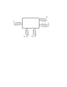
FIG. 2.: Representation of the measurement apparatus of Fig.1 as a $5$-port quantum network.

The amplifier of Figure 1 is now depicted as the $5$-port quantum network of Figure 2 which couples the $5$ dissipation lines $l$, $r$, $f$, $a$, $b$. The advantage of this new picture is that all noise sources are now attributed to free fields coming through the dissipation lines and are thus separated from the purely reactive elements gathered in the network. As a consequence, the transformation of fields by the reactive network is described by a unitary $5\times 5$ scattering matrix. We give below the resulting expressions for the output fields $l^{\rm out}$ and $r^{\rm out}$ in the signal and readout lines

$$l^{\rm out} = -l^{\rm in}+\sqrt{\frac{R_{0}}{R_{l}}}\left(a^{\rm in}-c^{\rm in}\right)$$ (23)

$$r^{\rm out} = -r^{\rm in}-2\frac{Z_{f}}{\sqrt{R_{r}R_{l}}}l^{\rm in}-2\sqrt{\frac{R_{f}}{R_{r}}}f^{\rm in}$$ (26)

$$+\left(1+\frac{Z_{f}}{R_{l}}-\frac{Z_{f}}{R_{0}}\right)\sqrt{\frac{R_{0}}{R_{r}}}a^{\rm in}$$

$$-\left(1+\frac{Z_{f}}{R_{l}}+\frac{Z_{f}}{R_{0}}\right)\sqrt{\frac{R_{0}}{R_{r}}}c^{\rm in}$$

The first relation describes the back-action noise induced by the measurement device on the signal line. Here, this noise is just the voltage noise source associated with the amplifier. We recall that $c^{\rm in}$ is in fact the conjugate of an input field $b^{\rm in}$ defined exactly as the other ones (see (21)). We do not discuss the back-action noise in more detail and concentrate the forthcoming discussion on the second relation which describes the added noise. Notice that equations (26) also allow to study the correlations between the output fields $l^{\rm out}$ and $r^{\rm out}$ or between these fields and the input ones. The terms complementing the unitarity scattering matrix may be found in [19].

In order to characterize the performance of the measurement device in terms of added noise, we introduce an estimator $\widehat{l}^{\rm in}$ of the signal $l^{\rm in}$ as it may be deduced from the knowledge of the meter readout $r^{\rm out}$

$$\widehat{l}^{\rm in} = -\frac{\sqrt{R_{r}R_{l}}}{2Z_{f}}r^{\rm out}$$ (27)

$$= l^{\rm in}+\frac{\sqrt{R_{l}}}{Z_{f}}\left(\frac{\sqrt{R_{r}}}{2}r^{\rm in}+\sqrt{R_{f}}f^{\rm in}\right)$$ (30)

$$-\frac{1}{2}\left(\frac{1}{Z_{f}}+\frac{1}{R_{l}}-\frac{1}{R_{0}}\right)\sqrt{R_{l}R_{0}}a^{\rm in}$$

$$+\frac{1}{2}\left(\frac{1}{Z_{f}}+\frac{1}{R_{l}}+\frac{1}{R_{0}}\right)\sqrt{R_{l}R_{0}}c^{\rm in}$$

The estimator $\widehat{l}^{\rm in}$ would be identical to the measured signal $l^{\rm in}$ in the absence of added fluctuations. Hence the noise added by the measurement device is described by the supplementary terms assigned respectively to Nyquist noises $r^{\rm in}$ and $f^{\rm in}$ in the readout and feedback lines as well as Nyquist noises $a^{\rm in}$ and $c^{\rm in}$ in the two lines representing amplification noises. Notice that proper fluctuations of $l^{\rm in}$ are included in the signal and not in the added noise.

The whole added noise is characterized by a spectrum obtained as a sum of the uncorrelated noise spectra associated with these Nyquist noises

$$\Sigma = \frac{R_{l}R_{r}}{4\left|Z_{f}\right|^{2}}\sigma_{rr}^{\rm in}+\frac{R_{l}R_{f}}{\left|Z_{f}\right|^{2}}\sigma_{ff}^{\rm in}$$ (33)

$$+\frac{R_{l}R_{0}}{4}\left|\frac{1}{Z_{f}}+\frac{1}{R_{l}}-\frac{1}{R_{0}}\right|^{2}\sigma_{aa}^{\rm in}$$

$$+\frac{R_{l}R_{0}}{4}\left|\frac{1}{Z_{f}}+\frac{1}{R_{l}}+\frac{1}{R_{0}}\right|^{2}\sigma_{bb}^{\rm in}$$

The Nyquist spectra are given by thermal equilibrium relations (7) with temperatures $T_{r}$, $T_{f}$, $T_{a}$ and $T_{b}$. The expression (33) allows us to evaluate the added noise for arbitrary values of the impedance parameters and of these noise temperatures. In particular the amplification noises are characterized by the three parameters $R_{0}$, $T_{a}$ and $T_{b}$.

When concentrating the discussion on ultimate sensitivity of the measurement apparatus, we see from (33) that it is wise to have the feedback impedance large enough so that only the effects of amplifier noises persist. Introducing the parameter

$$e^{\xi}=\sqrt{\frac{R_{l}}{R_{0}}}$$ (34)

we rewrite (30,33) under the simple forms

$$\widehat{l}^{\rm in} = l^{\rm in}+\sinh\xi\,a^{\rm in}+\cosh\xi\,c^{\rm in}$$ (35)

$$\Sigma = \sinh^{2}\xi\,\sigma_{aa}^{\rm in}+\cosh^{2}\xi\,\sigma_{bb}^{\rm in}$$ (36)

If the two temperatures $T_{a}$ and $T_{b}$ are fixed, the added noise is made minimal by choosing the parameter $\xi$ equal to zero, that is also by matching the values of the two impedance parameters $R_{0}$ and $R_{l}$. Notice that this is not a good solution for decreasing the back-action noise (see (26)). But this is the optimum as far as the criterium of minimizing added noise is privileged. Then, relations (36) are read as

$$\widehat{l}^{\rm in} = l^{\rm in}+c^{\rm in}$$ (37)

$$\Sigma = \sigma_{bb}^{\rm in}$$ (38)

Finally this added noise is still decreased by going to a temperature $T_{b}$ as low as possible. At the limit of a null temperature, we recover the optimum of $3\,{\rm dB}$ added noise which is the same as for phase-insensitive linear amplifiers [11].

In this letter, we have studied the quantum noise associated with an ideal operational amplifier used as a phase-insensitive measurement apparatus. We have given a description of this apparatus as a quantum network coupling $5$ lines associated with the signal and readout lines, with the feedback resistance and with the two lines representing voltage and current noises added by the amplifier. We have obtained an expression of the noise added by the measurement which depends on the various impedance parameters and on the corresponding noise temperatures. We have shown that the ultimate performance of the device is reached when the following conditions are met: large feedback impedance $Z_{f}$, impedance $R_{l}$ of the signal line matched to the parameter $R_{0}$ characterizing the amplification noises, null temperature for these amplification noises.

As argued in the Introduction, amplifiers play an important role in most real-life high-sensitivity measurements. Amplification with an infinite gain may be considered as the archetypal description of the transition from a microscopic quantum signal to a macroscopic classical readout [20]. Amplifiers are also involved in active stabilization techniques. The representation of the ideal operational amplifier as a quantum network helps to treat it as an element used in more sophisticated systems. Hence, the results presented in the present letter should open the way to a renewed analysis of quantum measurements with active devices.

Acknowledgements We thank Vincent Josselin, Fulvio Ricci, Pierre Touboul and Eric Willemenot for fruitful discussions.

REFERENCES

- [1] A. Einstein, Annalen der Physik 17 (1905) 549.
- [2] H. Nyquist, Phys. Rev. 32 (1928) 110.
- [3] H.B. Callen and T.A. Welton, Phys. Rev. 83 (1951) 34.
- [4] E.M. Lifshitz and L.P. Pitaevskii, “Landau and Lifshitz, Course of Theoretical Physics, Statistical Physics Part 2” (Butterworth-Heinemann, 1980) ch. VIII.
- [5] H. Heffner, Proc IRE 50 (1962) 1604.
- [6] H.A. Haus and J.A. Mullen, Phys. Rev. 128 (1962) 2407.
- [7] J.P. Gordon, L.R. Walker and W.H. Louisell, Phys. Rev. 130 (1963) 806.
- [8] C.M. Caves, Phys. Rev. D26 (1982) 1817.
- [9] R. Loudon and T.J. Shephered, Optica Acta 31 (1984) 1243.
- [10] J.P. Gordon, Proc. IRE (1962) 1898.
- [11] H. Takahasi, in “Advances in Communication Systems” ed. A.V. Balakrishnan (Academic, 1965) 227.
- [12] B. Yurke and J.S. Denker, Phys. Rev. A29 (1984) 1419.
- [13] C.W. Gardiner, IBM J. Res. Dev. 32 (1988) 127.
- [14] Y. Yamamoto, S. Machida, S. Saito, N. Imoto, T. Yanagawa, N. Kitagawa and G. Björk, in “Progress in Optics XXVIII” ed. E. Wolf (1990) 87.
- [15] S. Reynaud, A. Heidmann, E. Giacobino and C. Fabre in “Progress in Optics XXX” ed. E. Wolf (1992) 1.
- [16] J-M. Courty and S. Reynaud, Phys. Rev. A46 (1992) 2766.
- [17] P. Grangier, J-M. Courty and S. Reynaud, Opt. Commun. 89 (1992) 99.
- [18] V.B. Braginsky and F.Ya. Khalili, “Quantum Measurement” (Cambridge, 1992).
- [19] F. Grassia, Thèse de l’Université Paris 6 (1998).
- [20] M. Ozawa, preprint quant-ph/9710023 (1997).