Heisenberg picture operators in the stochastic wave function approach to open quantum systems.

Abstract

A fast simulation algorithm for the calculation of multitime correlation functions of open quantum systems is presented. It is demonstrated that any stochastic process which “unravels” the quantum Master equation can be used for the calculation of matrix elements of reduced Heisenberg picture operators, and thus for the calculation of multitime correlation functions, by extending the stochastic process to a doubled Hilbert space. The numerical performance of the stochastic simulation algorithm is investigated by means of a standard example.

I Introduction

The state of an open quantum system is conventionally described through a reduced density matrix $\rho(t)$ whose dynamics is given by a dissipative equation of motion – the quantum Master equation. From a numerical point of view this formalism has a major drawback: for a system whose state is described in a $N$-dimensional Hilbert space ${\cal H}$, the quantum Master equation is a set of $N(N+1)/2$ coupled differential equations. Hence the numerical evaluation of the quantum Master equation is in practice not feasible for large systems [1].

This difficulty does not arise in the stochastic wave function approach to open systems [2, 3, 4, 5, 6, 7, 8, 9]: Here, the state of an open quantum system is described by a stochastic wave function $\psi(t)\in{\cal H}$, i.e., by a $N-$dimensional state vector. The stochastic time evolution of $\psi(t)$ is either defined through a stochastic Schrödinger equation [8, 9] (which is a stochastic differential equation) or alternatively through a conditional transition probability $T[\psi,t|\psi_{0},t_{0}]$ [6, 7], which is the probability density of finding the system in the state $\psi$ at time $t\geq t_{0}$ under the condition that the system is in the state $\psi_{0}$ at time $t_{0}$. The connection to the density matrix formalism is made through the relation

$$\rho(t) = \int D\psi D\psi^{*}\int D\psi_{0}D\psi_{0}^{*}\;|\psi\rangle\langle\psi|\;$$ (2)

$$\times T[\psi,t|\psi_{0},t_{0}]P[\psi_{0},t_{0}],$$

where $P[\psi_{0},t_{0}]$ is the probability density of an ensemble of normalized pure states characterizing some initial density matrix $\rho_{0}$ and $D\psi D\psi^{*}$ is the Hilbert space volume element [6, 7]. The integrals extend over the Hilbert space ${\cal H}$. This relation ensures that one-time expectation values of any system operators are calculated correctly. Note that this condition alone does not uniquely specify a stochastic process. Diffusion type stochastic processes [8, 9] as well as piecewise deterministic jump processes [2, 3, 4, 5, 6, 7] have been proposed in the literature. A unique stochastic process can only be derived by making further assumptions such as specifying a certain measurement scheme [10, 11, 12].

Especially in quantum optical systems one-time expectation values of system observables are not the only measurable quantities: for example, the spectrum of fluorescence of a two level system is the Fourier transform of the two-time correlation function $\langle\!\langle\sigma^{+}(\tau)\sigma^{-}\rangle\!\rangle_{\rm s}$ in the stationary state, where $\sigma^{\pm}$ denote the pseudo spin operators of the system. Thus, for a complete description of open quantum systems it is necessary to introduce Heisenberg picture operators. In the density matrix formalism this concept is well understood [13]: Consider the quantum Master equation

$$\dot{\rho}(t)=L(t)\rho(t),$$ (3)

where the super-operator $L(t)$ is defined as

$$L(t)\rho(t) = -i\left[H(t),\rho(t)\right]$$ (5)

$$+\frac{1}{2}\sum_{i}\gamma_{i}\Big{\{}2J_{i}\rho(t)J_{i}^{\dagger}-J_{i}^{\dagger}J_{i}\rho(t)-\rho(t)J_{i}^{\dagger}J_{i}\Big{\}}.$$

The operator $H(t)$ is essentially the Hamiltonian of the isolated system which contributes to the coherent part of the dynamics, and the rates $\gamma_{i}$ and the Lindblad operators $J_{i}$ describe the dissipative coupling of the system to its environment through the $i$-th decay channel. The solution of eq. (3) with respect to the initial condition $\rho(t_{0})=\rho_{0}$ can be expressed for $t\geq t_{0}$ in terms of the propagation super-operator $V(t,t_{0})$ as [14]

$$\rho(t)=V(t,t_{0})\rho_{0},$$ (6)

where $V(t,t_{0})$ is the solution of the differential equation

$$\frac{d}{dt}V(t,t_{0})=L(t)V(t,t_{0}),$$ (7)

with the initial condition $V(t_{0},t_{0})=I$. For an arbitrary Schrödinger system operator $A$ the matrix elements of the reduced Heisenberg picture operator are defined as

$$A_{t}(\phi_{0},\psi_{0}) \equiv \langle\phi_{0},t_{0}|A(t)|\psi_{0},t_{0}\rangle$$ (8)

$$= \mbox{Tr}_{\rm sys}\Big{\{}AV(t,t_{0})|\psi_{0}\rangle\langle\phi_{0}|\Big{\}}.$$ (9)

Eq. (8) can be interpreted in the following way: for the calculation of the matrix element $A_{t}(\phi_{0},\psi_{0})$ start with the initial “density matrix” $|\psi_{0}\rangle\langle\phi_{0}|$ and propagate it up to the time $t$. Then calculate the expectation value of $A$ with respect to the propagated “density matrix”. However, since $|\psi_{0}\rangle\langle\phi_{0}|$ is in general not a positive matrix and thus not a true density matrix, it can not be characterized by a probability density $P[\psi_{0},t_{0}]$ of normalized pure states in ${\cal H}$ (cf. eq. (2). Hence a direct application of the stochastic wave function approach to the calculation of Heisenberg picture operators is not possible.

II Heisenberg picture operators in the stochastic wave function approach

In a closed system where the time evolution of states is given through the unitary propagator $U(t,t_{0})$ we can calculate arbitrary matrix elements $A_{t}(\phi_{0},\psi_{0})$ of a Heisenberg operator $A(t)$ in the following way (cf. fig. 1): propagate $\phi_{0}$ and $\psi_{0}$ to obtain $\phi=U(t,t_{0})\phi_{0}$ and $\psi=U(t,t_{0})\psi_{0}$, respectively and then evaluate the scalar product $\langle\phi|A|\psi\rangle$. This method is easily generalized to the calculation of matrix elements of a reduced Heisenberg picture operator, i.e., to open systems: Instead of propagating the state vectors $\phi_{0}\in{\cal H}$ and $\psi_{0}\in{\cal H}$ separately, we can construct a stochastic process in the doubled Hilbert space $\widetilde{\cal H}={\cal H}\oplus{\cal H}$ which propagates the normalized pair of state vectors $\theta_{0}=(\phi_{0},\psi_{0})^{\rm T}/\sqrt{2}\in\widetilde{\cal H}$ simultaneously in such a way that the following condition holds:

$$A_{t}(\phi_{0},\psi_{0})=2\int D\theta D\theta^{*}\langle\phi|A|\psi\rangle\widetilde{T}[\theta,t|\theta_{0},t_{0}],$$ (10)

where $\theta=(\phi,\psi)^{\rm T}$ and we introduced the conditional transition probability $\widetilde{T}$ for the stochastic process in the doubled Hilbert space $\widetilde{\cal H}$. Throughout this letter, the superscript T denotes the transpose of a vector. This condition states that matrix elements of arbitrary Heisenberg operators are calculated correctly. It is important to note that eq. (10) alone does not specify the stochastic time evolution in the doubled Hilbert space uniquely. In fact, each stochastic process which can be used to simulate the quantum Master equation (3) can be extended to the doubled Hilbert space and used for the calculation of the matrix elements of arbitrary Heisenberg picture operators. We will first demonstrate this for the piecewise deterministic jump process proposed in [2, 3, 4, 5, 6, 7] and then generalize the result. A derivation of the simulation algorithm for the stochastic time evolution in the doubled Hilbert space which is based on a microscopic system–reservoir model can be found in Ref. [15].

For the piecewise deterministic jump process the simulation algorithm reads as follows: 1) Start with the normalized state $\theta_{0}=(\phi_{0},\psi_{0})^{\rm T}/\sqrt{2}$ at $t_{0}$. 2) Draw a random number $\eta_{1}$ from a uniform distribution on $[0,1]$; this random number will determine the time of the first jump. 3) Propagate $\theta_{0}$ according to the Schrödinger-type equation

$$i\frac{d}{ds}\hat{\theta}(s)=\widetilde{H}_{\rm eff}(s)\hat{\theta}(s)$$ (11)

where the extensions of the Hamiltonian $H$ and Lindblad operators $J_{i}$ to the doubled Hilbert space are defined as

$$\widetilde{H}(s)=\left(\begin{array}[]{cc}H(s)&0\\ 0&H(s)\end{array}\right),\quad\widetilde{J}_{i}=\left(\begin{array}[]{cc}J_{i}&0\\ 0&J_{i}\end{array}\right),$$ (12)

and the non-Hermitian effective Hamiltonian is defined as

$$\widetilde{H}_{\rm eff}(s)=\widetilde{H}(s)-\frac{i}{2}\sum_{i}\gamma_{i}\widetilde{J}_{i}^{\dagger}\widetilde{J}_{i}.$$ (13)

4) The time $T_{1}$ of the first jump is determined by the condition

$$\eta_{1}=\|\hat{\theta}(T_{1})\|^{2}.$$ (14)

5) Select a particular type of jump with probability $\gamma_{i}w_{i}/\sum_{i}\gamma_{i}w_{i}$, where $w_{i}=\|\widetilde{J}_{i}\hat{\theta}(T_{1})\|^{2}$. The state of the system immediately after the first jump is given by

$$\theta(T_{1})=\widetilde{J}_{i}\hat{\theta}(T_{1})/\|\widetilde{J}_{i}\hat{\theta}(T_{1})\|.$$ (15)

6) Draw a second random number $\eta_{2}$ to determine the time $T_{2}$ of the next jump and propagate $\theta(T_{1})$ according to the differential equation (11) and so on until $s=t$. 7) The state of the system at time $t$ is given by

$$\theta(t)\equiv(\phi(t),\psi(t))^{\rm T}=\hat{\theta}(t)/\|\hat{\theta}(t)\|.$$ (16)

The matrix elements of the reduced Heisenberg picture operator $A(t)$ are then obtained by computing

$$A_{t}(\phi_{0},\psi_{0})=2\Big{\langle}\!\Big{\langle}\langle\phi(t)|A|\psi(t)\rangle\Big{\rangle}\!\Big{\rangle},$$ (17)

where the angular brackets $\langle\!\langle\cdots\rangle\!\rangle$ denote the average over the realizations of the stochastic process.

In order to show that this algorithm leads to the correct result, we introduce the density matrix

$$\widetilde{\rho}(t)=\left(\begin{array}[]{cc}\widetilde{\rho}_{11}(t)&\widetilde{\rho}_{12}(t)\\ \widetilde{\rho}_{21}(t)&\widetilde{\rho}_{22}(t)\end{array}\right)$$ (18)

on the doubled Hilbert space $\widetilde{\cal H}$ which is a solution of the extended quantum Master equation

$$\dot{\widetilde{\rho}}(t) = -i\left[\widetilde{H}(t),\widetilde{\rho}(t)\right]$$ (20)

$$+\frac{1}{2}\sum_{i}\gamma_{i}\Big{\{}2\widetilde{J}_{i}\widetilde{\rho}(t)\widetilde{J}_{i}^{\dagger}-\widetilde{J}_{i}^{\dagger}\widetilde{J}_{i}\widetilde{\rho}(t)-\widetilde{\rho}(t)\widetilde{J}_{i}^{\dagger}\widetilde{J}_{i}\Big{\}},$$

with the initial condition

$$\widetilde{\rho}(t_{0})=|\theta_{0}\rangle\langle\theta_{0}|\equiv\frac{1}{2}\left(\begin{array}[]{cc}|\phi_{0}\rangle\langle\phi_{0}|&|\phi_{0}\rangle\langle\psi_{0}|\\ |\psi_{0}\rangle\langle\phi_{0}|&|\psi_{0}\rangle\langle\psi_{0}|\end{array}\right).$$ (21)

By definition of the extended operators $\widetilde{H}$ and $\widetilde{J}_{i}$ each component $\widetilde{\rho}_{ij}(t)$ which is an operator on ${\cal H}$ is a solution of the original quantum Master equation (3). Since $\widetilde{\rho}_{21}(t)$ is a solution of eq. (3) with the initial condition $\widetilde{\rho}_{21}(t_{0})=|\psi_{0}\rangle\langle\phi_{0}|/2$ the matrix elements $A_{t}(\phi_{0},\psi_{0})$ of a reduced Heisenberg picture operator $A(t)$ can be written as (cf. eq. (8))

$$A_{t}(\phi_{0},\psi_{0})=2\mbox{Tr}_{\rm sys}\Big{\{}A\widetilde{\rho}_{21}(t)\Big{\}}.$$ (22)

Now consider a particular “unraveling” of the extended quantum Master equation (20) which is characterized by a conditional transition probability $\widetilde{T}[\theta,t|\theta_{0},t_{0}]$ in the doubled Hilbert space. For the density matrix $\widetilde{\rho}(t)$ we then obtain in analogy to eq. (2)

$$\widetilde{\rho}(t)=\int D\theta D\theta^{*}\;|\theta\rangle\langle\theta|\;\widetilde{T}[\theta,t|\theta_{0},t_{0}],$$ (23)

and hence for $\widetilde{\rho}_{21}(t)$

$$\widetilde{\rho}_{21}(t)=\int D\theta D\theta^{*}\;|\psi\rangle\langle\phi|\;\widetilde{T}[\theta,t|\theta_{0},t_{0}],$$ (24)

where $\theta=(\phi,\psi)^{\rm T}$. By inserting eq. (24) into eq. (22) we recover eq. (10). Thus we have shown that matrix elements of reduced Heisenberg picture operators are calculated correctly (i.e., eq. (10) holds) if the stochastic process in the doubled Hilbert space can be used to simulate the extended quantum Master equation (20). Since this is the case for the simulation algorithm presented above we have completed the proof.

It is important to note that the above proof does not rely on a specific “unraveling” of the quantum Master equation (20). On the contrary, it is valid for any stochastic process the covariance matrix (see eq. (23)) of which is governed by eq. (20).

III Multitime correlation functions

The simulation algorithm in the doubled Hilbert space can also be used for the calculation of multitime correlation functions. Consider for example the two-time correlation function

$$g(\phi_{0},t_{1},t_{2})=\langle\phi_{0},t_{0}|A(t_{2})B(t_{1})|\phi_{0},t_{0}\rangle,$$ (25)

where $t_{1}\leq t_{2}$. Here, the stochastic simulation algorithm would read as follows: 1) Start in the state $\phi_{0}$ at time $t_{0}$ and use the stochastic time evolution in the Hilbert space ${\cal H}$ to obtain the stochastic wave function $\phi(t_{1})$. 2) Propagate the state

$$\theta(t_{1})=(\phi(t_{1}),B\phi(t_{1}))^{\rm T}/\|(\phi(t_{1}),B\phi(t_{1}))\|$$ (26)

using the stochastic time evolution in the doubled Hilbert space to obtain the state vector $\theta(t_{2})=(\phi(t_{2}),\psi(t_{2}))^{\rm T}$. The multitime correlation function is then obtained by computing

$$g(\phi_{0},t_{1},t_{2})=\Big{\langle}\!\Big{\langle}\big{\|}\big{(}\phi(t_{1}),B\phi(t_{1})\big{)}\big{\|}^{2}\langle\phi(t_{2})|A|\psi(t_{2})\rangle\Big{\rangle}\!\Big{\rangle}.$$ (27)

The generalization of this scheme to the calculation of arbitrary time-ordered multitime correlation functions of the form

$$g(\phi_{0},t_{0},t_{1},...,t_{n},s_{1},...,s_{m})$$ (28)

$$= \langle{\phi_{0},t_{0}}|A_{1}(t_{1})\cdots A_{n}(t_{n})B_{m}(s_{m})\cdots B_{1}(s_{1})|{\phi_{0},t_{0}}\rangle,$$ (29)

where $t_{0}\leq\cdots\leq t_{n}$, and $t_{0}\leq s_{1}\leq\cdots\leq s_{m}$, and $A_{i}$ and $B_{i}$ are arbitrary system operators is straightforward: Order the set of times $\{t_{1},\cdots t_{n},s_{1},\cdots s_{m}\}$ and rename them $r_{i}$ such that $r_{1}<\cdots<r_{q}$ where $q$ is the number of distinct time points. Then define a set of Schrödinger operators $F_{l}$ and $G_{l}$ as

$$\left\{\begin{array}[]{cl}F_{l}=A_{i}^{\dagger},G_{l}=I,&\mbox{if $r_{l}=t_{i}\neq s_{j}$ for some $i$ and all $j$,}\\ G_{l}=I,F_{l}=B_{j},&\mbox{if $r_{l}=s_{j}\neq t_{i}$ for some $j$ and all $i$,}\\ G_{l}=A_{i}^{\dagger},F_{l}=B_{j},&\mbox{if $r_{l}=t_{i}=s_{j}$ for some $i$ and $j$}.\end{array}\right.$$ (30)

The multitime correlation function $g(\phi_{0},t_{0},t_{1},...,$ $t_{n},s_{1},...,s_{m})$ is then obtained in the following way:

1) Start with the state $\phi_{0}$ at time $t_{0}$ and propagate it up to the time $r_{1}$ to obtain $\phi(r_{1})$.

2) Propagate the state

$$\theta(r_{1})=\left(F_{1}\phi(r_{1}),G_{1}\phi(r_{1})\right)^{\rm T}/\|(F_{1}\phi(r_{1}),G_{1}\phi(r_{1}))\|$$ (31)

to obtain $\theta(r_{2})=(\phi(r_{2}),\psi(r_{2}))^{\rm T}$.

3) Jump to the state

$$\theta(r_{2})=\left(F_{2}\phi(r_{2}),G_{2}\psi(r_{2})\right)^{\rm T}/\|(F_{2}\phi(r_{2}),G_{2}\psi(r_{2}))\|$$ (32)

and propagate it up to $r_{3}$ and so on. $g(\phi_{0},t_{0},t_{1},...,t_{n},s_{1},...,s_{m})$ is then given by

$$g(\phi_{0},t_{0},t_{1},...,t_{n},s_{1},...,s_{m})=$$ (35)

$$\Big{\langle}\!\Big{\langle}\big{\|}\big{(}F_{1}\phi(r_{1}),G_{1}\phi(r_{1})\big{)}\big{\|}^{2}\big{\|}\big{(}F_{2}\phi(r_{2}),G_{2}\psi(r_{2})\big{)}\big{\|}^{2}\cdots$$

$$\times\big{\|}\big{(}F_{q-1}\phi(r_{q-1}),G_{q-1}\psi(r_{q-1})\big{)}\big{\|}^{2}\langle\phi(r_{q})|F_{q}^{\dagger}G_{q}|\psi((r_{q})\rangle\Big{\rangle}\!\Big{\rangle}.$$

It is important to note, that also for higher order correlation functions, we only have to propagate two state vectors.

Finally, let us remark that the choice of the initial condition (27) (or (31), respectively) is not unique. We can also multiply the operator $B$ by a constant $\varepsilon$ and define the state vector $\theta_{\varepsilon}(t_{1})$ as

$$\theta_{\varepsilon}(t_{1})=(\phi(t_{1}),\varepsilon B\phi(t_{1}))^{\rm T}/\|(\phi(t_{1}),\varepsilon B\phi(t_{1}))\|$$ (36)

and accordingly the correlation function $g(\phi_{0},t_{1},t_{2})$ as

$$g(\phi_{0},t_{1},t_{2})=$$ (38)

$$\frac{1}{\varepsilon}\Big{\langle}\!\Big{\langle}\big{\|}\big{(}\phi(t_{1}),\varepsilon B\phi(t_{1})\big{)}\big{\|}^{2}\langle\phi_{\varepsilon}(t_{2})|A|\psi_{\varepsilon}(t_{2})\rangle\Big{\rangle}\!\Big{\rangle},$$

where $\theta_{\varepsilon}(t_{2})=(\phi_{\varepsilon}(t_{2}),\psi_{\varepsilon}(t_{2}))^{\rm T}$ is obtained by propagating $\theta_{\varepsilon}(t_{1})$ according to the simulation algorithm in the doubled Hilbert space. Again, the unnormalized deterministic motion is governed by the equation of motion

$$i\frac{d}{dt}\hat{\phi}_{\varepsilon}(t) = H_{\rm eff}(t)\hat{\phi}_{\varepsilon}(t)$$ (39)

$$i\frac{d}{dt}\hat{\psi}_{\varepsilon}(t) = H_{\rm eff}(t)\hat{\psi}_{\varepsilon}(t)$$ (40)

but in the limit $\varepsilon\rightarrow 0$, we find

$$\|\hat{\theta}_{\varepsilon}(t)\| \rightarrow\| \hat{\phi}_{\varepsilon}(t)\|$$ (41)

$$w_{i}=\|\widetilde{J}_{i}\hat{\theta}_{\varepsilon}(T)\|^{2} \rightarrow \|J_{i}\hat{\phi}_{\varepsilon}(T)\|^{2},$$ (42)

and hence the jumps of the trajectory $\theta_{\varepsilon}(t)$ are completely governed by the jumps of $\phi_{\varepsilon}(t)$, which evolves according to the “usual” stochastic time evolution in ${\cal H}$ (cf. Eqs. (14) and (15)). In this limit we obtain a procedure first proposed by Dum et al. in Ref. [5], which is based on “probing the system with $\delta$ kicks” (see Appendix D of Ref.[5]). For further discussions of this method see for example the Refs. [16, 17, 18].

IV Numerical results

In order to investigate the numerical performance of our simulation algorithm, we compare it with the method proposed by Dum et al. in Ref. [5] and with an alternative method proposed by Dalibard et al. which is based on a decomposition of the stochastic trajectory into four sub-trajectories [2]. Note that all procedures are fully consistent with the quantum regression theorem [14, 19] and hence lead to the same result for the multitime correlation function. However, the numerical performance of the algorithms is quite different. We demonstrate this by means of a standard example of quantum optics – the calculation of the spectrum of resonance fluorescence of a two level system. In fig. 2 (a) – (c) we show the computational time necessary to achieve a given accuracy (measured by the relative error of the correlation function $\langle\!\langle\sigma^{+}(\tau)\sigma^{-}\rangle\!\rangle_{\rm s}$ in the stationary state) for a coherently driven two level atom with Rabi frequency $\Omega=10\gamma$ obtained on a RS6000 workstation. The solid lines represent the mean square deviation of the numerical solution from the exact solution [20] and the dashed lines show the mean estimated standard deviation of the numerical solution. Obviously, the latter quantity provides for all algorithms a very good measure of the accuracy of the numerical simulation. In fig. 2 (d) we compare the estimated standard deviation for the three algorithms. Obviously, the numerical performance of the algorithms proposed by Dum et. al. and our algorithm is quite similar, although the convergence of our algorithm is smoother. On the other hand, for a given accuracy the stochastic simulation in the doubled Hilbert space is by a factor of $3$ faster than the algorithm proposed in [2]. We expect this result to be even better for higher order correlation functions since for a multitime correlation function of the type of eq. (28) one has to propagate in general $4^{n+m-1}$ different state vectors in each realization using the method of Castin et. al, whereas in our approach it is only necessary to propagate two state vectors.

Let us briefly summarize the main results of this letter: We have shown that starting from a stochastic simulation algorithm for the quantum Master equation (3) it is possible to obtain a fast simulation algorithm for the calculation of matrix elements of arbitrary Heisenberg picture operators and time-ordered multitime correlation functions by making the substitutions

$$\psi\in{\cal H}\longrightarrow\theta\in\widetilde{\cal H},\quad H\longrightarrow\widetilde{H},\quad J_{i}\longrightarrow\widetilde{J}_{i},$$ (43)

i.e., we replace the stochastic wave function $\psi(t)$ by a stochastic wave function $\theta(t)$ in the doubled Hilbert space and extend accordingly the operators $H$ and $J_{i}$ which are present in the quantum Master equation to the doubled Hilbert space (cf. eq. (12)). We emphasize that these replacements can be done for any “unraveling” of the quantum Master equation, e.g., also for the quantum state diffusion model [8, 9]. The resulting stochastic process in the doubled Hilbert space is then similar to a process first proposed by Gisin in [21]. However, the latter process is only well defined, when the initial states $\phi_{0}$ and $\psi_{0}$ are non-orthogonal, i.e., if $\langle\phi_{0}|\psi_{0}\rangle\neq 0$. This problem does not occur in the ansatz presented here.

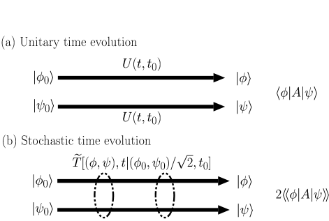
FIG. 1.: Calculation of Heisenberg operator matrix elements: (a) for a closed system and (b) for an open system.

FIG. 2.: Calculation of the first order correlation function $\langle\!\langle\sigma^{+}(\tau)\sigma^{-}\rangle\!\rangle_{\rm s}$ for a coherently driven two level atom on resonance. This figure shows the relative error vs. the CPU time in seconds for the simulation algorithms proposed in Ref. [2] (a), Ref. [5] (b), and for our algorithm in the doubled Hilbert space (c). The solid lines represent the mean square deviation of the numerical solution from the exact solution and the dashed lines show the estimated standard deviation of the numerical solution. In Fig. 2 (d), we compare the estimated standard deviation for the three algorithms.

REFERENCES

• [1] K. Mølmer, Y. Castin, and J. Dalibard, J. Opt. Soc. Am. B 10, 524 (1993).
• [2] J. Dalibard, Y. Castin, and K. Mølmer, Phys. Rev. Lett. 68, 580 (1992).
• [3] H. Carmichael, An Open Systems Approach to Quantum Optics, Lecture Notes in Physics m18 (Springer-Verlag, Berlin, Heidelberg, New York, 1993).
• [4] C. W. Gardiner, A. S. Parkins, and P. Zoller, Phys. Rev. A 46, 4363 (1992).
• [5] R. Dum, A. S. Parkins, P. Zoller, and C. W. Gardiner, Phys. Rev. A 46, 4382 (1992).
• [6] H. P. Breuer and F. Petruccione, Phys. Rev. Lett. 74, 3788 (1995).
• [7] H. P. Breuer and F. Petruccione, Phys. Rev. E 52, 428 (1995).
• [8] N. Gisin and I. C. Percival, J. Phys. A 25, 5677 (1992).
• [9] N. Gisin and I. C. Percival, J. Phys. A 26, 2233 (1993).
• [10] H. M. Wiseman and G. J. Milburn, Phys. Rev. A 47, 642 (1993).
• [11] H. M. Wiseman and G. J. Milburn, Phys. Rev. A 47, 1652 (1993).
• [12] H. P. Breuer and F. Petruccione, Fortschr. Phys. 45, 39 (1997).
• [13] R. Alicki and K. Lendi, Lecture Notes in Physics: Quantum Dynamical Semigroups and Applications (Springer-Verlag, Berlin, Heidelberg, New York, 1987).
• [14] C. W. Gardiner, Quantum Noise (Springer-Verlag, Berlin; Heidelberg, New York, 1991).
• [15] H. P. Breuer, B. Kappler, and F. Petruccione, Phys. Rev. A 56, 2334 (1997).
• [16] P. Marte, R. Dum, R. Taïeb, and P. Zoller, Phys. Rev. A 47, 1378 (1993).
• [17] P. Marte et al., Phys. Rev. Lett. 71, 1335 (1993).
• [18] K. Mølmer and Y. Castin, Quantum Semiclass. Opt. 8, 49 (1996).
• [19] D. F. Walls and G. J. Milburn, Quantum Optics (Springer-Verlag, Berlin, Heidelberg, New York, 1994).
• [20] B. R. Mollow, Phys. Rev. 188, 1969 (1969).
• [21] N. Gisin, J. mod. Optics 40, 2313 (1993).
Refer to caption