Stochastic wave function approach to the calculation of multitime correlation functions of open quantum systems

Abstract

Within the framework of probability distributions on projective Hilbert space a scheme for the calculation of multitime correlation functions is developed. The starting point is the Markovian stochastic wave function description of an open quantum system coupled to an environment consisting of an ensemble of harmonic oscillators in arbitrary pure or mixed states. It is shown that matrix elements of reduced Heisenberg picture operators and general time-ordered correlation functions can be expressed by time-symmetric expectation values of extended operators in a doubled Hilbert space. This representation allows the construction of a stochastic process in the doubled Hilbert space which enables the determination of arbitrary matrix elements and correlation functions. The numerical efficiency of the resulting stochastic simulation algorithm is investigated and compared with an alternative Monte Carlo wave function method proposed first by Dalibard et al. [Phys. Rev. Lett. 68, 580 (1992)]. By means of a standard example the suggested algorithm is shown to be more efficient numerically and to converge faster. Finally, some specific examples from quantum optics are presented in order to illustrate the proposed method, such as the coupling of a system to a vacuum, a squeezed vacuum within a finite solid angle, and a thermal mixture of coherent states.

I Introduction

In recent years several stochastic wave function methods have been developed and used to describe the dynamics of open quantum systems [1, 2, 3, 4, 5, 6, 7, 8]. All these approaches are based on the following idea: instead of solving the quantum master equation to obtain the time evolution of the reduced density matrix, an ensemble of pure states is propagated using a stochastic time evolution. This method provides two major advantages: the individual sample paths of the different realizations can – in some situations – be interpreted as the time evolution of an individual continuously monitored quantum system [9, 10, 11, 12] and the scaling of the numerical performance with the system size is better for this approach [1, 4, 5, 13, 14].

A particular interesting situation considered in quantum optics is the coupling of a system (e. g., an atom or a cavity) to the continuum of modes of the electromagnetic field. Since a lot of theoretical and experimental effort is used to prepare the environment in certain well defined states which are not restricted to thermal mixtures (see, e. g., [15, 16, 17]), it is interesting to investigate the time evolution of an open quantum system which is coupled to an environment in an arbitrary state. One way to obtain the stochastic time evolution of the reduced system takes as its starting point the quantum master equation for the reduced density matrix. A stochastic wave function is constructed on a phenomenological basis in the following way: start with an ensemble of pure states representing the initial density matrix $\rho(t_{0})=\rho_{0}$ and propagate each member of the ensemble using a stochastic time evolution which guarantees that the covariance matrix of the stochastic process is the reduced density matrix. This procedure ensures that expectation values of system observables are calculated correctly.

In applications of open quantum systems one is also interested in multitime correlation functions such as $\langle A(t+\tau)B(t)\rangle$, where $A(t+\tau)$ and $B(t)$ are Heisenberg operators, and the angular brackets denote the ensemble average. In the density matrix approach these quantities are usually determined by making use of the quantum regression theorem [18, 19] which is based on the identity

$$\langle A(t+\tau)B(t)\rangle$$ (1)

$$\hskip 30.00005pt=\mbox{Tr}_{\mbox{sys}}\bigg{\{}AV(t+\tau,t)\Big{\{}BV(t,t_{0})\left\{\rho_{0}\right\}\Big{\}}\bigg{\}},$$ (2)

where $\mbox{Tr}_{\mbox{sys}}$ denotes the trace over the system’s degrees of freedom and $V(t,t_{0})$ is the time evolution super operator of the corresponding quantum master equation, and $A$ and $B$ are Schrödinger operators. Eq. (1) allows the following interpretation: for the calculation of $\langle A(t+\tau)B(t)\rangle$ start with the density matrix $\rho(t_{0})=\rho_{0}$ and propagate to $\rho(t)$ using the quantum master equation. Then propagate the “density matrix” $B\rho(t)$ up to the time $t+\tau$ and calculate the quantum mechanical expectation value of $A$ with respect to this density matrix. However, since $B\rho(t)$ is, in general, not a positive matrix (and hence not a true density matrix), it can not be expressed as an ensemble of pure states and hence a direct generalization of this computational scheme to the stochastic wave function approach is not possible. Instead, some alternative computational schemes are proposed in the literature such as expressing time-ordered multitime correlation functions as the sum of symmetric time-ordered correlation functions [1] which can be simulated directly, or using the Heisenberg picture of the quantum state diffusion model [22].

In this article we will present a different approach to the derivation of the stochastic time evolution which is formulated within the framework of probability distributions on projective Hilbert space [7, 8]. The starting point for this approach is not the quantum Master equation for the reduced density matrix, but a microscopic model for the dynamics of the total system. This model is used to calculate the unitary time evolution of the total system in second order perturbation theory, which leads to a Liouville equation for the corresponding probability distribution. The equation of motion of the reduced system’s probability distribution is obtained by invoking a specific reduction formula, which relies upon the above stated condition that expectations of system operators are calculated accurately, and performing the Markov approximation. This scheme allows the derivation of the stochastic time evolution of an open quantum system coupled to an environment which is in an almost arbitrary state. To be more precise, the only restrictions we impose on the state of the environment concern the relative time scales of the system’s and the environment’s time evolution. Note, that this restriction is not fundamental but necessary in order to end up with a Markovian dynamics of the reduced system.

To construct a stochastic process that allows also the determination of multitime correlation functions we shall follow in this article the following strategy: multitime correlation functions are expressed in terms of matrix elements of reduced Heisenberg picture operators which can be written as expectation values in a doubled Hilbert space. This then enables the formulation of a stochastic process in the doubled Hilbert space which fulfills the condition, that matrix elements of reduced Heisenberg picture operators and hence multitime correlation functions are calculated correctly.

This article is organized as follows: In Sect. II we will briefly review the statistical description of quantum systems in terms of probability distributions on the underlying Hilbert space. Sec. III describes the derivation of the equation of motion of the reduced system’s probability density functional. We find that the time evolution of this probability density is governed by a Liouville–Master equation. The resulting stochastic process is thus a piecewise deterministic Markov process. In Sec. IV we define the matrix elements of the reduced Heisenberg picture operators. We show that these matrix elements can be determined by simulating a stochastic process in a doubled Hilbert space which is again a piecewise deterministic Markov process. The process defined in the doubled Hilbert space is used to calculate arbitrary measurable multitime correlation functions, which is shown in Sec. V. In order to illustrate the general theory presented in this article we explicitly discuss some examples of quantum optical systems in Sec. VI.

II Probability distributions on Hilbert space

The basis for a description of open quantum systems in terms of a stochastic wave function is the definition of a probability measure on the underlying Hilbert space ${\cal H}$. In this article we will make use of the probability density functional $P[\psi,t]$ which is defined such that $P[\psi,t]D\psi D\psi^{*}$ is the probability of finding the state of the system in the volume element $D\psi D\psi^{*}$ around $\psi$ at time $t$ [7, 8]. The volume element of the Hilbert space is defined as

$$D\psi D\psi^{*}\equiv\prod_{x}\frac{i}{2}d\psi(x)d\psi^{*}(x),$$ (3)

where $x$ labels a complete set of quantum numbers. Thus, the normalization of $P[\psi,t]$ reads

$$\int D\psi D\psi^{*}P[\psi,t]=1,$$ (4)

where the integral extends over the Hilbert space ${\cal H}$. In order to be consistent with the general principles of quantum mechanics we have to impose two further conditions on $P[\psi,t]$: i) since two state vectors which only differ by a phase factor describe the same physical state, we require that $P[\psi,t]$ does not depend on the phase of the state vector and ii) we are only interested in normalized state vectors, so that the support of $P[\psi,t]$ is the unit sphere in the Hilbert space ${\cal H}$. The quantum mechanical expectation value of an arbitrary linear operator $A$ with respect to $P[\psi,t]$ is defined as

$$\langle\!\langle A\rangle\!\rangle_{P[\cdot,t]}\equiv\int D\psi D\psi^{*}\langle\psi|A|\psi\rangle P[\psi,t].$$ (5)

For the composition of two statistically independent subsystems, which are described by two probability distributions $P_{1}$ and $P_{2}$ on the Hilbert spaces ${\cal H}_{1}$ and ${\cal H}_{2}$, respectively, we further define the tensor product probability distribution $P[\Psi,t]$ on ${\cal H}={\cal H}_{1}\otimes{\cal H}_{2}$ as [7, 8]

$$P[\Psi,t] = \int D\psi D\psi^{*}\int D\varphi D\varphi^{*}$$ (6)

$$\times \delta[\Psi-\psi\otimes\varphi]P_{1}[\psi,t]P_{2}[\varphi,t],$$ (7)

where $\delta[\cdot]$ is the functional delta distribution, and write as a short hand notation $P[\cdot,t]=P_{1}[\cdot,t]\otimes P_{2}[\cdot,t]$. The connection to the standard density matrix description of statistical ensembles is made through the identity

$$\rho_{t}(x,x^{\prime})\equiv\int D\psi D\psi^{*}\langle x|\psi\rangle\langle\psi|x^{\prime}\rangle P[\psi,t].$$ (8)

Hence, the density matrix is the covariance matrix of the stochastic process.

III Derivation of the equation of motion for the reduced system’s probability distribution

In this section we derive the equation of motion for the probability distribution of the states of an open system. To this end, we first describe briefly the class of models we want to treat (Sec. III A). We then introduce in Sec. III B the weak coupling assumption which enables us to derive an expression for the conditional transition probability $T[\psi,t+\tau|\psi_{0},t_{0}]$, where $\psi$, $\psi_{0}$ are pure states of the open system (Sec. III C 2). This result will be further simplified by making the Markov approximation (Sec. III D), and finally be used to obtain the desired equation of motion (Sec. III E).

A Description of the underlying model

Consider an open quantum system in the Hilbert space ${\cal H}_{1}$ with Hamiltonian $H_{1}$ interacting with an environment consisting of harmonic oscillators, e. g., the electromagnetic field modes. The pure states of the environment are elements of the Hilbert space ${\cal H}_{2}$ and the Hamiltonian $H_{2}$ of the environment is given by

$$H_{2}=\sum_{k}\omega_{k}b_{k}^{\dagger}b_{k},$$ (9)

where we set $\hbar=1$ for simplicity. Throughout this article, $b_{k}$ denotes the annihilation operator for the field mode $k=(\omega_{k},\hat{\mbox{\boldmath$k$}},\lambda_{k})$ with frequency $\omega_{k}$, unit wave vector $\hat{\mbox{\boldmath$k$}}$, and polarization index $\lambda_{k}$.

The initial condition for the state of the environment at time $t_{0}$ is given by a probability distribution

$$P_{2}[\varphi,t_{0}]=\sum_{\alpha}p_{\alpha}\int_{0}^{2\pi}\frac{d\chi}{2\pi}\delta[\varphi-e^{i\chi}\varphi_{\alpha}],$$ (10)

where the $p_{\alpha}$ are positive, normalized weights, i. e.,

$$p_{\alpha}\geq 0,\quad\sum_{\alpha}p_{\alpha}=1,$$ (11)

and the $\varphi_{\alpha}$ are arbitrary normalized states in ${\cal H}_{2}$. It is important to note that we do not suppose that the $\varphi_{\alpha}$ are orthogonal, i. e., the initial condition Eq. (10) also includes arbitrary mixtures of coherent states. We further assume that the system under consideration and the environment are statistically independent at time $t_{0}$, i. e., that the probability distribution of the total system factorizes at time $t_{0}$ (cf. Eq. (6)).

The interaction of the system with its environment is modeled via the interaction Hamiltonian

$$H_{I}=\sum_{i=1,2}A_{i}\otimes B_{i},$$ (12)

where the operators $A_{i}$ and $B_{i}$ are defined as

$$A_{1} = A,\quad A_{2}=A^{\dagger},$$ (13)

$$B_{1} = -i\sum_{k}g_{k}b_{k}^{\dagger},\quad B_{2}=B_{1}^{\dagger}.$$ (14)

The $g_{k}$ are the (real) coupling constants. For optical systems $A$ and $A^{\dagger}$ could be, for example, the positive and negative frequency part of the dipole operator. It is useful to assume that the $A_{i}$ are eigenoperators of $H_{1}$, i. e., $[H_{1},A_{i}]=\omega_{i}A_{i}$ with $\omega_{1}=-\omega_{s}$, and $\omega_{2}=\omega_{s}$, where $\omega_{s}$ is the system frequency. This is no restriction since this can always be achieved by choosing appropriate linear combinations of $A$ and $A^{\dagger}$. This type of coupling describes for example the interaction of a two level system or a harmonic oscillator with a quantized electromagnetic field in the rotating wave approximation, which is of particular interest in quantum optics. Note that the restriction to this kind of coupling has only technical reasons. The generalization of the presented theory to a coupling involving more than one system operator $A$, which was considered for example in Ref. [8], is straightforward. The Hamiltonian of the total system is

$$H=H_{1}+H_{2}+H_{I}.$$ (15)

In order to simplify the discussion in Sec. III D, where we state the conditions necessary to perform the Markov approximation, we will introduce at this point a decomposition of the Hilbert space of the environment into the Hilbert space ${\cal H}_{\mbox{B}}$ which is the state space of the bath and the Hilbert space ${\cal H}_{\mbox{Dr}}$ which describes the driving field. This decomposition reflects the fact that the electromagnetic field which interacts with the system is in general produced by different sources which can have totally different effects on the system. This decomposition is defined as follows:

Let ${\cal K}_{\mbox{B}}$ be the set of modes $k$ for which $\langle\!\langle b_{k}\rangle\!\rangle_{P_{2}[\cdot,t_{0}]}=0$, i. e., the modes which do not contribute to the average electromagnetic field and ${\cal K}_{\mbox{Dr}}$ be the set of modes $k$ for which $\langle\!\langle b_{k}\rangle\!\rangle_{P_{2}[\cdot,t_{0}]}\neq 0$. Then we define the Hilbert space of the bath ${\cal H}_{\mbox{B}}$ as

$${\cal H}_{\mbox{B}}=\bigotimes_{k\in{\cal K}_{\mbox{B}}}{\cal H}_{k},$$ (16)

where ${\cal H}_{k}$ is the Hilbert space of the field mode $k$, and similarly we define the Hilbert space ${\cal H}_{\mbox{Dr}}$ of the driving field. Obviously we have ${\cal H}_{2}={\cal H}_{\mbox{B}}\otimes{\cal H}_{\mbox{Dr}}$. We further assume that the states belonging to ${\cal H}_{\mbox{B}}$ and ${\cal H}_{\mbox{Dr}}$ are statistically independent, i. e., the probability distribution of the environment can be written as $P_{2}=P_{\mbox{B}}\otimes P_{\mbox{Dr}}$, where $P_{\mbox{B}}$ and $P_{\mbox{Dr}}$ are the probability distributions on the bath space and on the space of the driving field respectively. This assumption is reasonable since the two fields are usually generated by different and independent sources.

With the above definitions in mind we can decompose accordingly the operators $B_{i}$ as follows:

$$B_{i}=B_{i}^{\mbox{B}}\otimes I+I\otimes B_{i}^{\mbox{Dr}},$$ (17)

where

$$B_{1}^{\mbox{B}}=-i\sum_{k\in{\cal K}_{\mbox{B}}}g_{k}b_{k}^{\dagger},\quad B_{2}^{\mbox{B}}={B_{1}^{\mbox{B}}}^{\dagger},$$ (18)

and

$$B_{1}^{\mbox{Dr}}=-i\sum_{k\in{\cal K}_{\mbox{Dr}}}g_{k}b_{k}^{\dagger},\quad B_{2}^{\mbox{Dr}}={B_{1}^{\mbox{Dr}}}^{\dagger}.$$ (19)

For the expectations of the operators $B_{i}$ we thus obtain

$$\langle\!\langle B_{i}\rangle\!\rangle_{P_{2}[\cdot,t]}=\langle\!\langle B_{i}^{\mbox{Dr}}\rangle\!\rangle_{P_{\mbox{Dr}}[\cdot,t]},$$ (20)

i. e., the expectation of the electromagnetic field only depends on the state of the driving field and is independent of the state of the bath. For the two time correlation function $\langle\!\langle B_{i}^{\dagger}(s)B_{j}\rangle\!\rangle_{P_{2}[\cdot,t]}$, where $B_{i}(s)=\exp(iH_{2}s)B_{i}\exp(-iH_{2}s)$, we find

$$\langle\!\langle B_{i}^{\dagger}(s)B_{j}\rangle\!\rangle_{P_{2}[\cdot,t]} = \langle\!\langle{B_{i}^{\mbox{B}}}^{\dagger}(s)B_{j}^{\mbox{B}}\rangle\!\rangle_{P_{\mbox{B}}[\cdot,t]}$$ (21)

$$+ \langle\!\langle{B_{i}^{\mbox{Dr}}}^{\dagger}(s)B_{j}^{\mbox{Dr}}\rangle\!\rangle_{P_{\mbox{Dr}}[\cdot,t]},$$ (22)

which means that this correlation functions can be split into the sum of two terms, where the first term only depends on the state of the bath and the second term is due to the driving field.

B Dynamics of the environment – weak coupling assumption

The basis of the weak coupling assumption is the fact that the environment is large compared to the system. Hence it is assumed that the dynamics of the environment is given by its free time evolution; the perturbations due to the interaction with the system under consideration can be neglected. For the probability distribution of the environment this means

$$P_{2}\left[\varphi,t\right]=\sum_{\alpha}p_{\alpha}\int_{0}^{2\pi}\frac{d\chi}{2\pi}\delta\left[\varphi-e^{i\chi}e^{-iH_{2}(t-t_{0})}\varphi_{\alpha}\right]$$ (23)

for all $t$, and we have chosen the initial condition given in Eq. (10).

Using the weak coupling assumption, we can further evaluate the expressions for the bath correlation functions $\langle\!\langle{B_{i}^{\mbox{B}}}^{\dagger}(s)B_{j}^{\mbox{B}}\rangle\!\rangle_{P_{\mbox{B}}[\cdot,t]}$ defined in Sec. III A, if the states of the individual bath modes are statistically independent, which means that the probability distribution of the bath is the product of probability distributions $P_{k}$ on the Hilbert spaces ${\cal H}_{k}$ of the individual bath modes $k$. This will be the case for the examples we want to treat in this article. We obtain for example

$$\langle\!\langle{B_{2}^{\mbox{B}}}^{\dagger}(s)B_{2}^{\mbox{B}}\rangle\!\rangle_{P_{\mbox{B}}[\cdot,t]}=\sum_{k\in{\cal K}_{\mbox{B}}}g_{k}^{2}e^{i\omega s}\langle\!\langle b_{k}^{\dagger}b_{k}\rangle\!\rangle_{P_{k}[\cdot,t_{0}]}.$$ (24)

It is important to note, that this correlation function only depends on the time argument $s$ and the state of the bath at time $t_{0}$; it is independent of the time $t$.

C Dynamics of the reduced system

In this section we focus on the description of the dynamics of the reduced system evolving from the initial distribution of the total system

$$P[\cdot,t_{0}]=P_{1}[\cdot,t_{0}]\otimes P_{2}[\cdot,t_{0}]$$ (25)

(cf. Eq. (6) for the definition of the tensor product probability distribution), where

$$P_{1}[\psi,t_{0}]=\int_{0}^{2\pi}\frac{d\chi}{2\pi}\delta[\psi-e^{i\chi}\psi_{0}],$$ (26)

and $P_{2}[\varphi,t_{0}]$ is given by Eq. (10). Thus at time $t_{0}$ the system is in the pure state $\psi_{0}$ and the initial distribution of the environment is given by the probability distribution $P_{2}$. The dynamics of the reduced system is completely described through the conditional transition probability $T[\psi,t_{0}+\tau|\psi_{0},t_{0}]$, which is the probability that the system is in the state $\psi$ at time $t_{0}+\tau$ under the condition that the system is in the state $\psi_{0}$ at time $t_{0}$. In order to do this, we will start in Sec. III C 1 with the calculation of the time evolution of the pure product state $\Psi_{\alpha}(t_{0})=\psi_{0}\otimes\varphi_{\alpha}$ in second order perturbation theory. Using this result we can calculate $P[\Psi,t_{0}+\tau]$ and applying a reduction formula (Sec. III C 2), we finally obtain an exact expression for the conditional transition probability.

It is important to note that the conditional transition probability $T[\psi,t_{0}+\tau|\psi_{0},t_{0}]$ also defines the dynamics of the reduced system, if its initial state is given by an arbitrary probability distribution $P_{1}[\psi,t_{0}]$. According to the general laws of probability theory the propagated reduced probability distribution $P_{1}[\psi,t_{0}+\tau]$ given the conditional transition probability $T$ is

$$P_{1}[\psi,t_{0}+\tau]=\int D\psi_{0}D\psi_{0}^{*}T[\psi,t_{0}+\tau|\psi_{0},t_{0}]P_{1}[\psi_{0},t_{0}].$$ (27)

Thus it is sufficient to consider the initial conditions Eq. (26).

1 Time evolution of the total system in second order perturbation theory

In this section we will study the time evolution of the initial distribution Eq. (25) in second order perturbation theory. To this end, we have to calculate the time evolution of the pure product state $\Psi_{\alpha}(t_{0})=\psi_{0}\otimes\varphi_{\alpha}$. In the interaction picture which coincides with the Schrödinger picture at time $t_{0}$, the operators $A_{i}(\tau)$ are given by

$$A_{i}(\tau)=A_{i}e^{i\omega_{i}\tau},\quad i=1,2,$$ (28)

since $A_{i}$ is an eigenoperator of $H_{1}$, and the operators $B_{i}(\tau)$ are given by

$$B_{1}(\tau) = -i\sum_{k}g_{k}b_{k}^{\dagger}e^{i\omega_{k}\tau},$$ (29)

$$B_{2}(\tau) = i\sum_{k}g_{k}b_{k}e^{-i\omega_{k}\tau}.$$ (30)

In second order perturbation theory we obtain for the propagated state

$$|{\Psi_{\alpha}(t_{0}+\tau)}\rangle = |{\psi_{0}}\rangle\otimes|{\varphi_{\alpha}}\rangle+\sum_{i}A_{i}|{\psi_{0}}\rangle\otimes f_{i}|{\varphi_{\alpha}}\rangle$$ (31)

$$+ \sum_{i,j}A_{i}^{\dagger}A_{j}|{\psi_{0}}\rangle\otimes g_{ij}|{\varphi_{\alpha}}\rangle,$$ (32)

where the first and second order propagation operators acting on the states of the environment are

$$f_{i} = -i\int_{0}^{\tau}ds\;e^{i\omega_{i}s}B_{i}(s),$$ (33)

$$g_{ij} = -\int_{0}^{\tau}ds\int_{0}^{\tau-s}ds^{\prime}e^{-i\omega_{i}(s+s^{\prime})}e^{i\omega_{j}s}$$ (35)

$$\times B_{i}^{\dagger}(s+s^{\prime}){B_{j}}(s).$$

If we define the averages of $f_{i}$ and $g_{ij}$ with respect to the probability distribution of the environment as

$$F_{i}\equiv\langle\!\langle f_{i}\rangle\!\rangle_{P_{2}[\cdot,t_{0}]},\quad G_{ij}\equiv\langle\!\langle g_{ij}\rangle\!\rangle_{P_{2}[\cdot,t_{0}]},$$ (36)

and the shifted operators $\widetilde{f}_{i}$ and $\widetilde{g}_{ij}$ as

$$\widetilde{f}_{i}\equiv f_{i}-F_{i},\quad\widetilde{g}_{ij}\equiv g_{ij}-G_{ij},$$ (37)

we can rewrite Eq. (32) as

$$|{\Psi_{\alpha}(t_{0}+\tau)}\rangle = L|\psi_{0}\rangle\otimes|{\varphi_{\alpha}}\rangle+\sum_{i}A_{i}|{\psi_{0}}\rangle\otimes\widetilde{f}_{i}|{\varphi_{\alpha}}\rangle$$ (38)

$$+ \sum_{i,j}A_{i}^{\dagger}A_{j}|{\psi_{0}}\rangle\otimes\widetilde{g}_{ij}|{\varphi_{\alpha}}\rangle$$ (39)

where we introduced the time evolution operator $L$ which is defined as

$$L=I+\sum_{i}F_{i}A_{i}+\sum_{i,j}G_{ij}A_{i}^{\dagger}A_{j}.$$ (40)

As we will show in Sec. III C 2, Eq. (38) is the basis for the construction of a specific reduction formula.

We can also use Eq. (38) to determine the time evolution of the probability distribution of the total system if the initial probability distribution is given by Eq. (25). For the propagated distribution $P[\Psi,t_{0}+\tau]$ we simply obtain

$$P[\Psi,t_{0}+\tau]=\sum_{\alpha}p_{\alpha}\int_{0}^{2\pi}\frac{d\chi}{2\pi}\delta[\Psi-e^{i\chi}\Psi_{\alpha}(t_{0}+\tau)],$$ (41)

where the states $\Psi_{\alpha}(t_{0}+\tau)$ are the propagated states defined in Eq. (38).

2 Reduction formula

The key to the stochastic description of open quantum systems is the reduction formula [7, 8]. The reduction formula states how the conditional transition probability $T[\psi,t_{0}+\tau|\psi_{0},t_{0}]$ is defined given the probability distribution $P[\Psi,t]$ (cf. Eq. (41)) on the state space of the total system ${\cal H}_{1}\otimes{\cal H}_{2}$. In order to derive an appropriate expression for $T$ we require the following necessary condition to hold:

$$\int D\Psi D\Psi^{*}\langle\Psi|C\otimes I|\Psi\rangle P[\Psi,t_{0}+\tau]$$ (42)

$$\stackrel{{\scriptstyle!}}{{=}} \int D\psi D\psi^{*}\langle\psi|C|\psi\rangle T[\psi,t_{0}+\tau|\psi_{0},t_{0}],$$ (43)

or in the more compact notation introduced in Sec. II

$$\langle\!\langle C\otimes I\rangle\!\rangle_{P[\cdot,t_{0}+\tau]}\stackrel{{\scriptstyle!}}{{=}}\langle\!\langle C\rangle\!\rangle_{T[\cdot,t_{0}+\tau|\psi_{0},t_{0}]}.$$ (44)

Note that the integral on the left-hand side of Eq. (42) extends over the Hilbert space ${\cal H}_{1}\otimes{\cal H}_{2}$, whereas the integral on the right-hand side only extends over the reduced state space ${\cal H}_{1}$. The above condition ensures that the time evolution of the expectation value of an arbitrary operator $C\otimes I$ acting on the total system’s state space calculated using the distribution $P[\Psi,t_{0}+\tau]$ is the same as the expectation value of $C$ with respect to $T[\psi,t_{0}+\tau|\psi_{0},t_{0}]$. However, there are infinitely many ways to construct a reduced probability distribution which fulfills the above condition, just as there are infinitely many ways to express an arbitrary density matrix as an ensemble of pure states [23], and each reduced probability distribution will define a different stochastic process. In Ref. [12] it was shown that different processes can be formulated using different “reduction bases” (which are bases of the Hilbert space of the environment). These processes were interpreted as the time evolution of a continuously monitored individual quantum system and each process was related to a specific measurement scheme [10].

Here, we will follow a different approach, which has the advantage that it results in a particular simple, basis-free reduction formula, but which is not based on a specific measurement scheme. If we insert the propagated probability distribution of the total system Eq. (41) in the left-hand side of the consistency condition Eq. (44) and neglect terms of the order $g_{k}^{3}$ we obtain

$$\langle\!\langle C\otimes I\rangle\!\rangle_{P[\cdot,t_{0}+\tau]} = \langle{\psi_{0}}|L^{\dagger}CL|{\psi_{0}}\rangle$$ (46)

$$+\sum_{i,j}\Gamma_{ij}\langle{\psi_{0}}|A_{i}^{\dagger}CA_{j}|{\psi_{0}}\rangle,$$

where we introduced the $(2\times 2)$–correlation matrix of the environment

$$\Gamma_{ij}=\langle\!\langle\widetilde{f}_{i}^{\dagger}\widetilde{f}_{j}\rangle\!\rangle_{P_{2}[\cdot,t_{0}]}=-(G_{ij}+G_{ji}^{*}+F_{i}^{*}F_{j}),$$ (47)

and $F_{i}$ and $G_{ij}$ are defined in Eq. (36). Note that $\Gamma$ is Hermitian and non-negative. If we denote the normalized eigenvectors of $\Gamma$ by ${\mu}_{i}=(\mu_{1i},\mu_{2i})^{T}$, and its eigenvalues by $\widetilde{\lambda}_{i}$, and define the system (jump-) operators as

$$J_{i}=\sum_{k}\mu_{ki}^{*}A_{k},$$ (48)

then Eq. (46) can be written as

$$\langle\!\langle C\otimes I\rangle\!\rangle_{P[\cdot,t_{0}+\tau]} = \langle{\psi_{0}}|L^{\dagger}CL|{\psi_{0}}\rangle$$ (50)

$$+\sum_{i}\widetilde{\lambda}_{i}\langle{\psi_{0}}|J_{i}^{\dagger}CJ_{i}|{\psi_{0}}\rangle$$

$$\stackrel{{\scriptstyle!}}{{=}} \langle\!\langle C\rangle\!\rangle_{T[\cdot,t_{0}+\tau|\psi_{0},t_{0}]}.$$ (51)

Consider the following conditional transition probability:

$$T[\psi,t_{0}+\tau|\psi_{0},t_{0}] = w\delta[\psi-w^{-1/2}L\psi_{0}]$$ (52)

$$+ \sum_{i}\tilde{\lambda}_{i}w_{i}\delta[\psi-w_{i}^{-1/2}J_{i}\psi_{0}],$$ (53)

where $w=||L{\psi_{0}}||^{2}$, and $w_{i}=||J_{i}{\psi_{0}}||^{2}$. Obviously, the conditional transition probability defined by Eq. (52) satisfies the necessary condition Eq. (44). Since in the generic case the matrix $\Gamma$ is nondegenerated we find three contributions to $T$: the system can evolve into the state $w^{-1/2}L\psi_{0}$, or to one of the two states $w_{1}^{-1/2}J_{1}\psi_{0}$, and $w_{2}^{-1/2}J_{2}\psi_{0}$. Note, that the expression for the conditional transition probability Eq. (52) is exact within second order perturbation theory; however, its derivation is based on the special choice of the initial probability distribution Eq. (25) and the complete dynamics of the environment is contained in the functions $w$, $w_{i}$, $\widetilde{\lambda}_{i}$, and the operators $L$, and $J_{i}$.

D The Markov approximation

In Sec. III C 2 we derived an expression for the conditional transition probability $T[\psi,t_{0}+\tau|\psi_{0},t_{0}]$ (cf. Eq. (52)) which is exact within second order perturbation theory. However, in situations where the environment has a large number of degrees of freedom, this formula is of little practical use for computations without further approximations. The simplest approximation scheme resulting in a conditional transition probability which is independent of the actual state of the environment, is the Markov approximation. We will use this approximation to calculate the quantities involving the state of the environment, namely the ensemble average of the first order propagation operator $F_{i}$ (cf. Eqs. (33) and (36)) and the ensemble average of the second order propagation operator $G_{ij}$ (cf. Eqs. (35), and (36)). This will be done in Sec. III D 1 and Sec. III D 2, respectively. These results will then be combined in Sec. III D 3 in order to establish an approximate expression for the conditional transition probability.

1 Calculation of the ensemble average of the first order propagation operator

We can simply calculate the ensemble average $F_{i}$ of the first order propagation operator $f_{i}$ (cf. Eq. (33)) by Taylor expansion. To first order in $\tau$ we obtain:

$$F_{1}=-\tau{\cal E}_{t_{0}}^{*},\quad F_{2}=\tau{\cal E}_{t_{0}},$$ (54)

where ${\cal E}_{t_{0}}$ is the mean electromagnetic field at time $t_{0}$, weighted with respect to the coupling constants $g_{k}$, and the probability distribution $P_{2}[\cdot,t_{0}]$. Using Eq. (20) we find

$${\cal E}_{t_{0}}=-i\langle\!\langle B_{2}\rangle\!\rangle_{P_{2}[\cdot,t_{0}]}=\sum_{k\in{\cal K}_{\mbox{Dr}}}g_{k}\langle\!\langle b_{k}\rangle\!\rangle_{P_{\mbox{Dr}}[\cdot,t_{0}]}.$$ (55)

Obviously, the quantities $F_{i}$ only depend on the driving field and are independent of the state of the bath. However, the validity of this approximation is limited to the validity of the Taylor expansion to first order in $\tau$, and this is guaranteed by the condition

$$\tau\ll\tau_{\cal E},$$ (56)

where $\tau_{\cal E}$ is the correlation time of the mean electromagnetic field; this correlation time is of the order of magnitude of the inverse bandwidth of the spectrum of the driving field.

2 Calculation of the ensemble average of the second order propagation operator

Performing a Taylor expansion of Eq. (35) with respect to $\tau$ in order to calculate the ensemble average of the second order propagation operator $G_{ij}$ we are lead to a vanishing first order term, i. e., $G_{ij}$ is at least quadratic in $\tau$. However, this Taylor expansion is only valid for a propagation time $\tau$ which is small compared to the decay time of the correlation function of the environment $\langle\!\langle B_{i}^{\dagger}(s)B_{j}\rangle\!\rangle_{P_{2}[\cdot,t_{0}]}$. Since this correlation function is the sum of the correlation function of the bath and the driving field (cf. Eq. (21)), we find that $G_{ij}$ is the sum of two terms, where the first one depends only on the state of the bath, and the second depends only on the state of the driving field, i. e.,

$$G_{ij}=G_{ij}^{\mbox{B}}+G_{ij}^{\mbox{Dr}}.$$ (57)

Since we focus our interest on situations, where the decay time $\tau_{\mbox{B}}$ of the bath correlation is very small compared to the decay time $\tau_{\mbox{Dr}}$ of the driving field correlation (which is equal to $\tau_{\cal E}$ for a coherent driving field) and to the time scale $\tau_{s}$ of the systematic dynamics, we have to use an appropriate approximation of $G_{ij}$ for “medium” values of $\tau$, i. e., for values of $\tau$ for which

$$\tau_{\mbox{B}}\ll\tau\ll\tau_{\mbox{Dr}},\tau_{\cal E},\tau_{s}.$$ (58)

In this case, the bath correlation function leads to a contribution $G_{ij}^{\mbox{B}}$ linear in $\tau$ whereas the driving field correlation function leads to a term $G_{ij}^{\mbox{Dr}}$ which is quadratic in $\tau$; thus we will neglect the latter. By describing the dynamics of the open system on a coarse grained time axis, i. e., by neglecting time variations which are smaller than $\tau_{\mbox{B}}$ we can perform the Markov approximation and extend the range of the integration over $s^{\prime}$ in Eq. (35) to infinity. The result to first order in $\tau$ is

$$G_{ij}=-\tau\int_{0}^{\infty}ds\;e^{-i\omega_{i}s}\langle\!\langle{B_{i}^{\mbox{B}}}^{\dagger}(s)B_{j}^{\mbox{B}}\rangle\!\rangle_{P_{\mbox{B}}[\cdot,t_{0}]}.$$ (59)

We can simplify this further by evaluating the above integral, as shown in Appendix  A. The result is:

$$G_{11} = -\tau\left(\frac{\gamma}{2}\left(N+1\right)-i\left(S_{0}+S_{1}\right)\right)$$ (60)

$$G_{12} = \tau\frac{\gamma}{2}Me^{2i\omega_{s}t_{0}}$$ (61)

$$G_{21} = \tau\frac{\gamma}{2}M^{*}e^{-2i\omega_{s}t_{0}}$$ (62)

$$G_{22} = -\tau\left(\frac{\gamma}{2}N+iS_{1}\right).$$ (63)

If the individual bath modes are statistically independent then the real constants $N$ and $S_{1}$, and the complex constant $M$ do not depend on the time $t_{0}$. This would not be the case if some bath modes with different frequencies were not statistically independent.

3 Conditional transition probability in Markov approximation

In this section, we will combine the results of Sec. III C 2, where we derived an exact expression for the time evolution of the conditional transition probability, with the approximations developed in Secs. III D 1 and III D 2, to obtain the short time dynamics of the conditional transition probability in Markov approximation.

We shall begin with the evaluation of the correlation matrix of the environment $\Gamma$: inserting Eqs. (54) and (60) into Eq. (47), we find to first order in $\tau$

$$\Gamma=\gamma\tau\left(\begin{array}[]{cc}N+1&-Me^{2i\omega_{s}t_{0}}\\ -M^{*}e^{-2i\omega_{s}t_{0}}&N\end{array}\right).$$ (64)

By computing the eigenvalues $\widetilde{\lambda}_{i}$ and the corresponding normalized eigenvectors ${\mu}_{i}$ of $\Gamma$, we obtain using Eq. (48) the jump operators $J_{i}$. (In order to simplify the notation, we do not write the $t_{0}$–dependency of $\widetilde{\lambda}_{i}$ and ${\mu}_{i}$ explicitly.)

Furthermore, we can calculate the operator $L$, which describes the smooth time evolution of the reduced system, by inserting Eqs. (54) and (60) into Eq. (40). The result to first order in $\tau$ is

$$L=I-i\tau\Big{(}H_{\mbox{Dr}}(t_{0})+H_{\rm LS}(t_{0})+H_{\rm D}(t_{0})\Big{)},$$ (65)

where the three operators $H_{\mbox{Dr}}(t_{0})$, $H_{\rm LS}(t_{0})$, and $H_{\rm D}(t_{0})$, which account for the influence of the environment on the open system are defined below. We can distinguish the effects of the two sources of the electromagnetic field:

1. The driving field: Using Eq. (54) we find

$$\frac{i}{\tau}\sum_{i}F_{i}A_{i}=i{\cal E}_{t_{0}}A^{\dagger}-i{\cal E}_{t_{0}}^{*}A=:H_{\mbox{Dr}}(t_{0}).$$ (66)

This is precisely the operator, which has to be added to the Hamiltonian of a quantum system in the presence of a classical electromagnetic field (according to the principle of minimal substitution) or a coherent driving field [24]. However, this result is also true for more general driving fields, since the only assumptions we have to make about the nature of the driving field concern its correlation times $\tau_{\cal E}$ and $\tau_{\mbox{Dr}}$ (cf. Secs. III D 1 and III D 2).

2. The bath: Using Eq. (60) we find

$$\frac{i}{\tau}\sum_{ij}G_{ij}A_{i}^{\dagger}A_{j}=:H_{\rm LS}(t_{0})+H_{\rm D}(t_{0}),$$ (67)

where

$$H_{\rm LS}=-(S_{0}+S_{1})A^{\dagger}A+S_{1}AA^{\dagger}$$ (68)

is a Hermitian operator which leads to small energy shifts – the Lamb shift $S_{0}$ and the Stark shift $S_{1}$. The non-Hermitian operator

$$H_{\rm D}(t_{0}) = -i\frac{\gamma}{2}\bigg{(}(N+1)A^{\dagger}A+NAA^{\dagger}$$ (69)

$$- M^{*}AAe^{2i\omega_{s}t_{0}}-Me^{-2i\omega_{s}t_{0}}A^{\dagger}A^{\dagger}\bigg{)}$$ (70)

describes the damping due to the coupling to the bath. If we define $\lambda_{i}=\widetilde{\lambda}_{i}/\gamma\tau$, then the damping operator can also be written as

$$H_{\rm D}(t_{0})=-i\frac{\gamma}{2}\sum_{i}\lambda_{i}J_{i}^{\dagger}J_{i}.$$ (71)

Using Eq. (71) and the fact that $H_{\rm D}(t_{0})$ is the only non-Hermitian operator which contributes to the operator $L$, it is clear that the weight $w=||L\psi_{0}||^{2}$ is given by

$$w=1-\gamma\tau\sum_{i}\lambda_{i}\langle{\psi_{0}}|J_{i}^{\dagger}J_{i}|{\psi_{0}}\rangle=1-\gamma\tau\sum_{i}\lambda_{i}w_{i}.$$ (72)

The latter equality ensures that $w+\gamma\tau\sum_{i}\lambda_{i}w_{i}=1$, which is equivalent to the normalization of the conditional transition probability.

Summing up the above results and transforming back to the Schrödinger picture, we finally obtain the conditional transition probability in the Markov approximation

$$T[\psi,t_{0}+\tau|\psi_{0},t_{0}] = \left(1-\gamma\tau\sum_{i}\lambda_{i}||J_{i}\psi_{0}||^{2}\right)$$ (73)

$$\times \delta\left[\psi-\left(I-i\tau G\left(t_{0}\right)\right)\psi_{0}\right]$$ (74)

$$+ \gamma\tau\sum_{i}\lambda_{i}||J_{i}\psi_{0}||^{2}\delta\left[\psi-\frac{J_{i}\psi_{0}}{||J_{i}\psi_{0}||}\right].$$ (75)

Here, we introduced the nonlinear time evolution operator [7, 8]

$$G(t_{0})\psi_{0}=\left(H_{\rm eff}(t_{0})+i\frac{\gamma}{2}\sum_{i}\lambda_{i}||J_{i}\psi_{0}||^{2}\right)\psi_{0},$$ (76)

and the effective system Hamiltonian

$$H_{\rm eff}(t_{0})=H_{1}(t_{0})+H_{\mbox{Dr}}(t_{0})+H_{\rm LS}+H_{\rm D}(t_{0}).$$ (77)

Note, that the deterministic propagation with the nonlinear operator $G(t_{0})$ conserves the norm of the propagated state and thus confines the dynamics to the unit sphere of the Hilbert space of the system.

The following comment may be helpful. If we combine the two approximations we made (second order perturbation theory and the Markov approximation) with the weak coupling assumption and assume that the probability distribution $P[\Psi,t_{0}]$ of the total system factorizes at time $t_{0}$, i. e., $P[\cdot,t_{0}]=P_{1}[\cdot,t_{0}]\otimes P_{2}[\cdot,t_{0}]$, then the probability distribution $P[\Psi,t_{0}+\tau]$ of the total system at time $t_{0}+\tau$ can be approximated by

$$P[\cdot,t_{0}+\tau]=P_{1}[\cdot,t_{0}+\tau]\otimes P_{2}[\cdot,t_{0}+\tau],$$ (78)

where $P_{1}[\cdot,t_{0}+\tau]$ is given by Eqs. (27) and (73) and $P_{2}[\cdot,t+\tau]$ by Eq. (23), i. e., $P[\cdot,t_{0}+\tau]$ approximately factorizes. Thus we can use the same scheme for the calculation of the conditional transition probability $T[\widetilde{\psi},t_{0}+\tau+\tau^{\prime}|{\psi},t_{0}+\tau]$ and by repeating this argument, we find that $P[\cdot,t]$ factorizes for all $t$. Hence, the dynamics of the reduced system is Markovian.

E Equation of motion for the reduced probability distribution

One possible starting point for the derivation of the differential equation of motion for the reduced probability distribution is the infinitesimal generator $\cal G$ of the process [25], which is defined by its action on an arbitrary functional $R$, which may depend explicitly on time:

$${\cal G}R[\psi_{0},t_{0}]=\lim_{\tau\rightarrow 0}\frac{{\cal P}_{\tau}R[\psi_{0},t_{0}]-R[\psi_{0},t_{0}]}{\tau},$$ (79)

where the propagator ${\cal P}_{\tau}$ is defined by

$${\cal P}_{\tau}R[\psi_{0},t_{0}]=\int D\psi D\psi^{*}R[\psi,t_{0}+\tau]T[\psi,t_{0}+\tau|\psi_{0},t_{0}],$$ (80)

i. e., ${\cal P}_{\tau}R[\psi_{0},t_{0}]$ is the expectation value of the functional $R$ at time $t_{0}+\tau$ under the condition that the process starts in the state $\psi_{0}$ at time $t_{0}$. Inserting Eqs. (73) and (80) in Eq. (79) and performing the limit $\tau\rightarrow 0$ on the coarse grained time axis (i. e., $\tau\gg\tau_{\mbox{B}}$) we obtain

$${\cal G}R[\psi_{0},t_{0}] = i\int dx\bigg{(}(G(t_{0})\psi_{0})^{*}(x)\frac{\delta R[\psi_{0},t_{0}]}{\delta\psi_{0}^{*}(x)}$$ (81)

$$- \frac{\delta R[\psi_{0},t_{0}]}{\delta\psi_{0}(x)}(G(t_{0})\psi_{0})(x)\bigg{)}$$ (82)

$$+ \int D\psi^{*}D{\psi}(R[\psi,t_{0}]-R[\psi_{0},t_{0}])W[{\psi}|\psi_{0},t_{0}],$$ (83)

where we defined the transition functional

$$W[{\psi}|\psi_{0},t_{0}]=\gamma\sum_{i}\lambda_{i}\langle{\psi_{0}}|J_{i}^{\dagger}J_{i}|{\psi_{0}}\rangle\delta\left[\psi-\frac{J_{i}\psi_{0}}{||J_{i}{\psi_{0}}||}\right].$$ (84)

Note, that the $t_{0}$–dependency of $W[{\psi}|\psi_{0},t_{0}]$ is given through $\lambda_{i}$ and $J_{i}$. Eq. (81) represents the generator of a piecewise deterministic Markov process [26], whose sample paths consist of deterministically propagated pieces interrupted by stochastic jumps. The deterministic pieces are the solution of the nonlinear Schrödinger equation [7, 8]

$$i\frac{d}{dt}\psi(t)=G(t)\psi(t),$$ (85)

and the waiting time distribution function for the stochastic jumps is given by [7, 8]

$$F[\psi_{0},t_{0},t]=1-\exp\left(-\gamma\sum_{i}\lambda_{i}\int_{t_{0}}^{t}ds||J_{i}\psi(s)||^{2}\right).$$ (86)

This is the probability that a jump occurs in the time interval $[t_{0},t)$ under the condition that the system is in the state $\psi_{0}$ at time $t_{0}$. If a jump occurs at time $T$ then the state of the system at time $T$ is

$$|{\psi(T)}\rangle=\frac{J_{i}|{\psi(T_{-})}\rangle}{||J_{i}|{\psi(T_{-})}\rangle||}$$ (87)

with probability $w_{i}/(w_{1}+w_{2})$, where $T_{-}$ is $\lim_{\epsilon\rightarrow 0}(T-\epsilon)$, with $\epsilon>0$.

In order to obtain the differential equation of motion for the reduced probability distribution, we set $R[\psi^{\prime},t]=\delta[\psi-\psi^{\prime}]$ and obtain

$${\cal P}_{\tau}R[\psi^{\prime},t]=T[\psi,t+\tau|\psi^{\prime},t],$$ (88)

and thus

$$\frac{\partial}{\partial t}P_{1}[\psi,t] = \lim_{\tau\rightarrow 0}\frac{1}{\tau}\Big{(}P_{1}[\psi,t+\tau]-P_{1}[\psi,t]\Big{)}$$ (89)

$$= \lim_{\tau\rightarrow 0}\int D\psi^{\prime}D{\psi^{\prime}}^{*}\frac{T[\psi,t+\tau|\psi^{\prime},t]-\delta[\psi-\psi^{\prime}]}{\tau}P_{1}[\psi^{\prime},t]$$ (90)

$$= \int D\psi^{\prime}D{\psi^{\prime}}^{*}\Big{(}{\cal G}\delta[\psi-\psi^{\prime}]\Big{)}P_{1}[\psi^{\prime},t].$$ (91)

If we insert Eq. (81) in Eq. (89) and evaluate the integral we obtain the differential equation of motion of the reduced probability distribution

  

$$\frac{\partial}{\partial t}P_{1}[\psi,t] = i\int dx\left\{\frac{\delta}{\delta\psi(x)}\Big{(}G(t)\psi\Big{)}(x)-\frac{\delta}{\delta\psi^{*}(x)}\Big{(}G(t)\psi\Big{)}^{*}(x)\right\}P_{1}[\psi,t]$$ (92)

$$+ \int D{\psi^{\prime}}D{\psi^{\prime}}^{*}\Big{\{}W[\psi|{\psi^{\prime},t}]P_{1}[{\psi^{\prime}},t]-W[{\psi^{\prime}}|\psi,t]P_{1}[\psi,t]\Big{\}}$$ (93)

which is a Liouville–Master Equation [7, 8]. Eq. (92) implies that for the conditional transition probability the integro-differential equation

$$\frac{\partial}{\partial t}T[\psi,t|\psi_{0},t_{0}] = i\int dx\left\{\frac{\delta}{\delta\psi(x)}\Big{(}G(t)\psi\Big{)}(x)-\frac{\delta}{\delta\psi^{*}(x)}\Big{(}G(t)\psi\Big{)}^{*}(x)\right\}T[\psi,t|\psi_{0},t_{0}]$$ (94)

$$+ \int D{\psi^{\prime}}D{\psi^{\prime}}^{*}\Big{\{}W[\psi|{\psi^{\prime}},t]T[\psi^{\prime},t|\psi_{0},t_{0}]-W[{\psi^{\prime}}|\psi,t]T[\psi,t|\psi_{0},t_{0}]\Big{\}}$$ (95)

holds for any $t>t_{0}$. This equation can be solved either analytically for some simple systems using the Hilbert–space path integral representation of the process [12, 27] or numerically by either simulating the process [7, 8] or using a recursive computation scheme [26].

IV Reduced Heisenberg picture operators

Studying the dynamics of open systems, one is not only interested in the time evolution of expectation values of some system operator $X$ but, moreover, one wants to investigate the time evolution of an arbitrary matrix element of this operator and obtain quantities such as $\langle{\phi_{0},t_{0}}|X(\tau)|{\psi_{0},t_{0}}\rangle$. Note that for an open system this is only a short hand notation. What we really mean by this is

$$\langle{\phi_{0},t_{0}}|X(\tau)|{\psi_{0},t_{0}}\rangle$$ (96)

$$\hskip 30.00005pt\equiv\sum_{\alpha}p_{\alpha}\langle{\Phi_{\alpha},t_{0}}|e^{iH\tau}\left(X\otimes I\right)e^{-iH\tau}|{\Psi_{\alpha},t_{0}\rangle},$$ (97)

where $H$ is the Hamiltonian of the total system (see Eq. (15)) and the states $\Phi_{\alpha}$ and $\Psi_{\alpha}$ are defined as $\Phi_{\alpha}=\phi_{0}\otimes\varphi_{\alpha}$ and $\Psi_{\alpha}=\psi_{0}\otimes\varphi_{\alpha}$, i. e., we assume, that the state of the environment is given by the probability distribution Eq. (10). We will refer to this quantity (Eq. (96)) as the matrix element of the reduced Heisenberg picture operator $X(\tau)$ and use it in Sec. V B 2 for the calculation of time-ordered multitime correlation functions.

In the case of a closed system, $\langle{\phi_{0},t_{0}}|X(\tau)|{\psi_{0},t_{0}}\rangle$ is easily calculated by solving the corresponding Schrödinger equation with the two initial conditions $\phi(t_{0})=\phi_{0}$ and $\psi(t_{0})=\psi_{0}$ separately to obtain $\phi(t_{0}+\tau)$ and $\psi(t_{0}+\tau)$ and then evaluating the scalar product $\langle{\phi(t_{0}+\tau)}|X|{\psi(t_{0}+\tau)}\rangle$. A naive generalization of this scheme to an open system – which will lead to wrong results – would be the following: instead of solving the Schrödinger equation, simulate the stochastic process defined in Sec. III E with the two initial conditions $\phi_{0}$ and $\psi_{0}$ to obtain $\phi(t_{0}+\tau)$ and $\psi(t_{0}+\tau)$. Then evaluate the scalar product $\langle{\phi(t_{0}+\tau)}|X|{\psi(t_{0}+\tau)}\rangle$ and average over a sufficiently large ensemble of realizations. However, what we really obtain using this procedure is the quantity

$$f(\phi_{0},\psi_{0},t_{0},\tau) = \int D\phi D\phi^{*}\int D\psi D\psi^{*}\langle{\phi}|X|{\psi}\rangle$$ (98)

$$\times T[\phi,t_{0}+\tau|\phi_{0},t_{0}]T[\psi,t_{0}+\tau|\psi_{0},t_{0}],$$ (99)

which is, in general, not equal to $\langle{\phi_{0},t_{0}}|X(\tau)|{\psi_{0},t_{0}}\rangle$. This can be most easily seen by considering the special case $\phi_{0}=\psi_{0}$: According to the definition of the conditional transition probability (cf. Sec. III C 2), $T[\psi,t_{0}+\tau|\psi_{0},t_{0}]$ has to fulfill the necessary condition

$$\langle{\psi_{0},t_{0}}|X(\tau)|{\psi_{0},t_{0}}\rangle = \int D\psi D\psi^{*}\langle{\psi}|X|{\psi}\rangle$$ (100)

$$\times T[\psi,t_{0}+\tau|\psi_{0},t_{0}].$$ (101)

Obviously, the quantity $f(\psi_{0},\psi_{0},t_{0},\tau)$ defined in Eq. (98) is, in general, different from the right-hand side of Eq. (100), and thus this approach will lead to wrong results.

However, as we will show below, it is possible to construct a stochastic process which describes the time evolution of $\phi_{0}$ and $\psi_{0}$ simultaneously and whose sample paths can be used to estimate the desired quantity $\langle{\phi_{0},t_{0}}|X(\tau)|{\psi_{0},t_{0}}\rangle$. In order to do so, we describe the dynamics of the open system in the doubled Hilbert space $\widetilde{\cal H}_{1}={\cal H}_{1}\oplus{\cal H}_{1}$, such that the “state” of the open system is given by a normalized pair of state vectors $\theta=c^{-1/2}(\phi,\psi)^{T}$, where $c=||\phi||^{2}+||\psi||^{2}$ and $T$ denotes the transposed vector. Accordingly, we define the extension of a system operator $X$ to the doubled Hilbert space $\widetilde{\cal H}_{1}$ as

$$\widetilde{X}=\left(\begin{array}[]{cc}I&0\\ 0&X\end{array}\right).$$ (102)

Using the raising operator

$$S^{+}=\left(\begin{array}[]{cc}0&I\\ 0&0\end{array}\right),$$ (103)

whose expectation value $c\langle\theta|S^{+}|\theta\rangle$ in the state $\theta$ is the scalar product $\langle\phi|\psi\rangle$, we can write the matrix elements of $X$ as

$$\langle{\varphi}|X|{\psi}\rangle=c\langle{\theta}|{\widetilde{X}}^{\dagger}S^{+}\widetilde{X}|{\theta}\rangle.$$ (104)

This equation is the crucial point of the following construction: it allows to write matrix elements of reduced system operators as expectation values in the doubled Hilbert space $\widetilde{\cal H}_{1}$. The same idea will be used in Sec. V B 2 for the development of an algorithm that enables the determination of arbitrary correlation functions. Note, that the scalar products on the left-hand side and on the right-hand side of the above equations are defined in different Hilbert spaces, namely in ${\cal H}_{1}$ and $\widetilde{\cal H}_{1}$, respectively. (The ${\widetilde{X}}^{\dagger}$ on the right-hand side of Eq. (104) is introduced to highlight the connection of the above equation with Eq. (150) (see below)). We also introduce a reduced probability distribution $\widetilde{P}_{1}[\theta,t]$ on the set of normalized states of $\widetilde{\cal H}_{1}$, which is the probability density of finding the system in the state $\theta$, and a conditional transition probability $\widetilde{T}[\theta,t_{0}+\tau|\theta_{0},t_{0}]$ which is the probability density that the system is in the state $\theta$ at time $t_{0}+\tau$ under the condition that the system is in the state $\theta_{0}$ at time $t_{0}$.

The goal of this section is to derive in analogy to the scheme we presented in Sec. III the equation of motion for the conditional transition probability $\widetilde{T}$, which has to fulfill the necessary condition

$$\langle{\phi_{0},t_{0}}|X(\tau)|{\psi_{0},t_{0}}\rangle=c_{0}\langle\!\langle{\widetilde{X}}^{\dagger}S^{+}\widetilde{X}\rangle\!\rangle_{\widetilde{T}[\cdot,t_{0}+\tau|\theta_{0},t_{0}]},$$ (105)

where $c_{0}=||\phi_{0}||^{2}+||\psi_{0}||^{2}$ and $\theta_{0}={c_{0}}^{-1/2}(\phi_{0},\psi_{0})^{T}$. The above condition states that the matrix element $\langle{\phi_{0},t_{0}}|X(\tau)|{\psi_{0},t_{0}}\rangle$ of a reduced Heisenberg picture operator is proportional to the expectation value of the operator ${\widetilde{X}}^{\dagger}S^{+}\widetilde{X}$ with respect to the probability distribution $\widetilde{T}$. In order to achieve this we have to make the following assumptions, which are similar to those made in Sec. III: i) According to the weak coupling assumption, we will assume that the time evolution of the environment is given by its free evolution (cf. Eq. (23)). ii) The probability distribution of the total system at time $t_{0}$, $\widetilde{P}[\Theta,t_{0}]$ (which is defined on the Hilbert space $\widetilde{\cal H}=\widetilde{\cal H}_{1}\otimes{\cal H}_{2}$), factorizes and is given by

$$\widetilde{P}[\Theta,t_{0}]=\sum_{\alpha}p_{\alpha}\int_{0}^{2\pi}\frac{d\chi}{2\pi}\delta[\Theta-e^{i\chi}\theta_{0}\otimes\varphi_{\alpha}].$$ (106)

iii) Second order perturbation theory and finally iv) the Markov approximation. If we combine these approximations we find after some calculations which are similar to those presented in Sec. III, that the necessary condition Eq. (105) to first order in $\tau$ (and to second order in the coupling $g_{k}$) reads:

$$\langle{\phi_{0},t_{0}}|X(\tau)|{\psi_{0},t_{0}}\rangle = \langle{\phi_{0}}|L^{\dagger}XL|{\psi_{0}}\rangle$$ (107)

$$+ \gamma\tau\sum_{i}\lambda_{i}\langle{\phi_{0}}|J_{i}^{\dagger}XJ_{i}|{\psi_{0}}\rangle$$ (108)

$$\stackrel{{\scriptstyle!}}{{=}} c_{0}\langle\!\langle{\widetilde{X}}^{\dagger}S^{+}\widetilde{X}\rangle\!\rangle_{\widetilde{T}[\cdot,t_{0}+\tau|\theta_{0},t_{0}]},$$ (109)

where $L$, and $\lambda_{i}$, and $J_{i}$ are defined as in Sec. III D 3. Note that this equation is completely analogous to Eq. (50). This leads us directly to a conditional transition probability to first order in $\tau$

$${\widetilde{T}[\theta,t_{0}+\tau|\theta_{0},t_{0}]} = \widetilde{w}\delta[\theta-\widetilde{w}^{-1/2}\widetilde{L}\theta_{0}]$$ (110)

$$+ \gamma\tau\sum_{i}\lambda_{i}\widetilde{w}_{i}\delta[\theta-\widetilde{w}_{i}^{-1/2}\widetilde{J}_{i}\theta_{0}],$$ (111)

where we have defined

$$\widetilde{H}_{\rm eff}(t)=\left(\begin{array}[]{cc}H_{\rm eff}(t)&0\\ 0&H_{\rm eff}(t)\end{array}\right),\quad\widetilde{J}_{i}=\left(\begin{array}[]{cc}J_{i}&0\\ 0&J_{i}\end{array}\right).$$ (112)

The effective Hamiltonian $H_{\rm eff}(t)$ is defined in Eq. (77), and $\widetilde{L}=I-i\tau\widetilde{H}_{\rm eff}$. The appropriate normalization constants are $\widetilde{w}=||\widetilde{L}\theta_{0}||^{2}$ and $\widetilde{w}_{i}=||\widetilde{J}_{i}\theta_{0}||^{2}$. In analogy to Eq. (72) we find

$$\widetilde{w}=1-\gamma\tau\sum_{i}\lambda_{i}||\widetilde{J}_{i}\theta_{0}||^{2}=1-\gamma\tau\sum_{i}\lambda_{i}\widetilde{w}_{i},$$ (113)

which ensures the normalization of the conditional transition probability $\widetilde{T}$.

The equation of motion for the conditional transition probability $\widetilde{T}[\theta,t|\theta_{0},t_{0}]$, where $t>t_{0}$, can be found using the same scheme as described in Sec. III E: Calculation of the generator ${\cal G}$ and its action on the functional $R[\theta^{\prime},t]=\delta[\theta-\theta^{\prime}]$ leads to the Liouville–Master equation

$$\frac{\partial}{\partial t}\widetilde{T}[\theta,t|\theta_{0},t_{0}] = i\int dx\bigg{\{}\frac{\delta}{\delta\theta(x)}\cdot\Big{(}\widetilde{G}(t)\theta\Big{)}(x)-\frac{\delta}{\delta\theta^{*}(x)}\cdot\Big{(}\widetilde{G}(t)\theta\Big{)}^{*}(x)\bigg{\}}\widetilde{T}[\theta,t|\theta_{0},t_{0}]$$ (114)

$$+ \int D{\theta^{\prime}}D{\theta^{\prime}}^{*}\Big{\{}W[\theta|\theta^{\prime},t]\widetilde{T}[\theta^{\prime},t|\theta_{0},t_{0}]-W[\theta^{\prime}|\theta,t]\widetilde{T}[\theta,t|\theta_{0},t_{0}]\Big{\}},$$ (115)

where we defined the functional Wirtinger derivative with respect to states belonging to $\widetilde{\cal H}_{1}$ as

$$\frac{\delta}{\delta\theta(x)}=\left(\begin{array}[]{c}\displaystyle\frac{\delta}{\delta\phi(x)}\\[8.61108pt] \displaystyle\frac{\delta}{\delta\psi(x)}\end{array}\right).$$ (116)

The generator for the continuous time evolution is defined in analogy to Eq. (76) as

$$\widetilde{G}(t)\theta=\left(\widetilde{H}_{\rm eff}(t)+i\frac{\gamma}{2}\sum_{i}\lambda_{i}||\widetilde{J}_{i}\theta||^{2}\right)\theta,$$ (117)

and the transition functional is given by (cf. Eq. (84))

$$W[\theta|\theta_{0},t]=\gamma\sum_{i}\lambda_{i}\widetilde{w}_{i}\delta\left[\theta-\widetilde{w}_{i}^{-1/2}\widetilde{J}_{i}\theta_{0}\right].$$ (118)

Again, the stochastic process which is defined through Eq. (114) is a piecewise deterministic Markov process, where the deterministic pieces are the solution of the nonlinear Schrödinger equation

$$i\frac{d}{dt}\theta=\widetilde{G}(t)\theta$$ (119)

and the waiting time distribution for the stochastic jumps under the condition that the system is in the state $\theta_{0}$ at time $t_{0}$ is given by

$$F[\theta_{0},t_{0},t]=1-\exp\left(-\gamma\sum_{i}\lambda_{i}\int_{t_{0}}^{t}ds||\widetilde{J}_{i}\theta(s)||^{2}\right).$$ (120)

The Liouville-Master equation (114) also determines the equation of motion for the reduced Heisenberg picture operator $X(t)$: Expanding $X(t)$ in terms of its matrix elements and inserting the Liouville-Master equation (114) we obtain after some calculations

$$\frac{d}{dt}X(t)=i[H_{1}+H_{\rm LS}+H_{\rm Dr},X](t)+\frac{1}{2}\sum_{i}\gamma_{i}$$ (121)

$$\times \Big{\{}2\left(J_{i}^{\dagger}XJ_{i}\right)(t)-\left(J_{i}^{\dagger}J_{i}X\right)(t)-\left(XJ_{i}^{\dagger}J_{i}\right)(t)\Big{\}}.$$ (122)

Thus the equation of motion of the reduced Heisenberg picture operator is the adjoint equation of the quantum master equation [20, 21] and we find

$$\mbox{Tr}_{\mbox{sys}}\Big{\{}XV(t,t_{0})\{\rho_{0}\}\Big{\}}=\mbox{Tr}_{\mbox{sys}}\Big{\{}X(t)\{\rho_{0}\}\Big{\}}$$ (123)

for any initial density matrix $\rho_{0}$, where $V(t,t_{0})$ is the time evolution super operator of the quantum master equation. This relation is the basis of the quantum regression theorem [18, 19].

We close this section with a few remarks: For the initial condition $\theta_{0}=(\psi_{0},\psi_{0})^{T}/\sqrt{2}$ the stochastic process defined in this way reduces to the stochastic process defined in Sec. III E; formally, this can be expressed through the identity

$$\widetilde{T}[\theta,t|\theta_{0},t_{0}]=\delta\left[\theta-\frac{1}{\sqrt{2}}(\psi,\psi)^{T}\right]T[\psi,t|\psi_{0},t_{0}],$$ (124)

where $T[\psi,t|\psi_{0},t_{0}]$ is the solution of the Liouville–Master equation (92). Thus, the dynamics of the system described in the doubled Hilbert space $\widetilde{\cal H}_{1}$ reduces to our earlier description of the dynamics in the ordinary Hilbert space ${\cal H}_{1}$. This is an important property of the conditional transition probability $\widetilde{T}$ which establishes the link between the two approaches.

For the numerical simulation of the stochastic process, it is useful to omit the normalization requirement and use the linear operator $\widetilde{H}_{\rm eff}$ instead of $\widetilde{G}$ as the generator for the deterministic motion. Thus, for the numerical simulation we use an unnormalized state vector $\hat{\theta}$, and the deterministic pieces are the solution of the linear Schrödinger-type equation

$$i\frac{d}{dt}\hat{\theta}=\widetilde{\cal H}_{\rm eff}\hat{\theta}$$ (125)

and the waiting time distribution for the stochastic jumps for unnormalized states is given by

$$F[\theta_{0},t_{0},t]=1-||\hat{\theta}(t)||^{2},$$ (126)

under the condition that the state $\theta_{0}$ is normalized and $\hat{\theta}(t)$ is the solution of the above Schrödinger-type equation with the initial condition $\hat{\theta}(t_{0})=\theta_{0}$. This equation is easily proven by differentiating Eqs. (120) and (126) with respect to $t$ and comparing the results. The above procedure has the major advantage, that the Schrödinger equation (125) for $\hat{\theta}=(\hat{\phi},\hat{\psi})$ is linear and that the two components are decoupled. This leads to a large reduction of the time necessary for the calculation of the deterministic time evolution. In addition, we do not have to calculate the waiting time distribution separately.

In Ref. [22] Gisin formulated the Heisenberg picture of the quantum state diffusion model of open systems. In analogy to our approach, he used a coupled pair of stochastic differential equations for the calculation of Heisenberg picture operators. His approach has the advantage that the scalar product of two state vectors $\phi$ and $\psi$ is constant in time, i. e., the matrix elements of the identity operator are calculated correctly in each realization of the stochastic process, whereas in our approach the identity operator is treated like any other system operator, i. e., for the calculation of the matrix elements one has to average over many realizations. On the other hand, Gisin’s approach is limited to the calculation of matrix elements with respect to nonorthogonal state vectors, i. e., the stochastic differential equations are not defined if $\langle\phi|\psi\rangle=0$. Furthermore, the quasi linear stochastic equations proposed for the numerical simulation, are not decoupled – in contrast to our approach – which is a disadvantage from a numerical point of view.

V Calculation of multitime correlation functions

A Symmetric time-ordered multitime correlation functions

The theory we presented in Sec. III allows the calculation of one time expectation values of an observable such as $\langle{\psi_{0},t_{0}}|X(\tau)|{\psi_{0},t_{0}}\rangle$. This theory can easily be extended to the calculation of symmetric, time-ordered multitime correlation functions such as

$$g(\psi_{0},t_{0},t_{1},t_{2})=\langle{\psi_{0},t_{0}}|X^{\dagger}(t_{1})Y(t_{2})X(t_{1})|{\psi_{0},t_{0}}\rangle,$$ (127)

where $X$ and $Y$ are arbitrary operators and $t_{0}\leq t_{1}\leq t_{2}$. As in Sec. IV we use the short hand notation

$$\langle{\psi_{0},t_{0}}|X^{\dagger}(t_{1})Y(t_{2})X(t_{1})|{\psi_{0},t_{0}}\rangle$$ (128)

$$\equiv \sum_{\alpha}p_{\alpha}\langle{\Psi_{\alpha},t_{0}}|X^{\dagger}(t_{1})Y(t_{2})X(t_{1})|{\Psi_{\alpha},t_{0}}\rangle,$$ (129)

where ${\Psi_{\alpha}}=\psi_{0}\otimes\varphi_{\alpha}$ is a pure product state of the total system. Thus, at time $t_{0}$ the system is in the pure state $\psi_{0}$ and the state of the environment is given through the probability distribution $P_{2}$ (cf. Eq. (10)). An exact expression for $g(\psi_{0},t_{0},t_{1},t_{2})$ in terms of probability distributions defined on the Hilbert space of the total system can be written as

$$g(\psi_{0},t_{0},t_{1},t_{2}) = \int D\Psi_{1}D\Psi_{1}^{*}\int D\Psi_{2}D\Psi_{2}^{*}\langle{\Psi_{2}}|Y|{\Psi_{2}}\rangle$$ (130)

$$\times \langle{\Psi_{1}}|X^{\dagger}X|{\Psi_{1}}\rangle\hat{T}\bigg{[}\Psi_{2},t_{2}\bigg{|}\frac{X\Psi_{1}}{||X\Psi_{1}||},t_{1}\bigg{]}P[\Psi_{1},t_{1}].$$ (131)

The time-dependent probability distribution $\hat{P}$ and the conditional transition probability $\hat{T}$ for the total system can be calculated using the unitary time evolution,

$$P[\Psi_{1},t_{1}]=\sum_{\alpha}p_{\alpha}\delta[\Psi_{1}-\exp(-iH(t_{0}-t_{1}))\psi_{0}\otimes\varphi_{\alpha}]$$ (132)

$$\hat{T}[\Psi_{2},t_{2}|\Psi_{1},t_{1}]=\delta[\Psi_{2}-\exp(-iH(t_{2}-t_{1}))\Psi_{1}],$$ (133)

where $H$ is the Hamilton of the total system (cf. Eq (15)). If we apply the scheme we presented in Sec. III (i. e., the weak coupling assumption, second order perturbation theory, the reduction formula, and the Markov approximation) to express $P$ and $\hat{T}$ in terms of the conditional transition probability $T$ of the reduced system we find that $g(\psi_{0},t_{0},t_{1},t_{2})$ is approximately given by

$$g(\psi_{0},t_{0},t_{1},t_{2}) = \int D\psi_{1}D\psi_{1}^{*}\int D\psi_{2}D\psi_{2}^{*}\langle{\psi_{2}}|Y|{\psi_{2}}\rangle$$ (134)

$$\times ||X\psi_{1}||^{2}\;T\bigg{[}\psi_{2},t_{2}\bigg{|}\frac{X\psi_{1}}{||X\psi_{1}||},t_{1}\bigg{]}T[\psi_{1},t_{1}|\psi_{0},t_{0}],$$ (135)

where the $\psi_{i}$ are states of the system under consideration and the conditional transition probability $T$ satisfies the Liouville–Master Equation Eq. (94). For the stochastic process which is used to simulate Eq. (134) this means the following: the process starts in the state $\psi_{0}$ at time $t_{0}$ and is propagated to the state $\psi_{1}$ at time $t_{1}$ using the stochastic time evolution defined in Sec. III C 2. Then the process jumps to the normalized state $X\psi_{1}/||X\psi_{1}||$ and is propagated to the state $\psi_{2}$ at time $t_{2}$.

For the most general symmetric time-ordered correlation function we obtain in a similar way

  

$$g(\psi_{0},t_{0},...,t_{n},t_{n+1}) = \langle{\psi_{0},t_{0}}|X_{1}^{\dagger}(t_{1})\cdots X_{n}^{\dagger}(t_{n})Y(t_{n+1})X_{n}(t_{n})\cdots X_{1}(t_{1})|{\psi_{0},t_{0}}\rangle$$ (136)

$$= \int D\psi_{1}D\psi_{1}^{*}\cdots\int D\psi_{n+1}D\psi_{n+1}^{*}\langle{\psi_{n+1},t_{n+1}}|Y|{\psi_{n+1},t_{n+1}}\rangle w_{1}\cdots w_{n}\times$$ (137)

$$\times T[\psi_{n+1},t_{n+1}|{w_{n}}^{-1/2}X_{n}\psi_{n},t_{n}]\cdots T[\psi_{2},t_{2}|{w_{1}}^{-1/2}X_{1}\psi_{1},t_{1}]T[\psi_{1},t_{1}|\psi_{0},t_{0}],$$ (138)

where $X_{i}$ and $Y$ are arbitrary system operators, and $w_{i}=||X_{i}\psi_{i}||^{2}$, and $t_{0}\leq t_{1}\leq\cdots\leq t_{n+1}$. This class of correlation functions contains for example the correlation $\langle{\sigma^{+}(t)\sigma^{+}(t+\tau)\sigma^{-}(t+\tau)\sigma^{-}(t)}\rangle$ which has been measured in the famous Hanbury-Brown and Twiss experiment (see, e. g. [28]) or, more recently, for a single ion in a trap by Diedrich and Walther [29].

The stochastic simulation algorithm which we use to compute symmetric time-ordered multitime correlation functions can thus be summarized as follows: 1. Start in the state $\psi_{0}$ at time $t_{0}$ and propagate up to the state $\psi_{1}$ at time $t_{1}$ using the stochastic time evolution (cf. Sec. III E). 2. Jump to the state $X_{1}\psi_{1}/||X_{1}\psi_{1}||$. 3. Propagate the state $X_{1}\psi_{1}/||X_{1}\psi_{1}||$ at time $t_{1}$ up to the time $t_{2}$, etc. 4. Compute the expectation value $\langle\psi_{n+1},t_{n+1}|Y|\psi_{n+1},t_{n+1}\rangle$. By repeating this procedure sufficiently often, we can estimate the unknown correlation function by averaging over the sample paths.

In the preceding discussion we limited ourselves to a pure initial state $\psi_{0}$ of the system. However, this is not a real restriction: if the initial state of the open system is described by a probability distribution $P_{1}[\psi,t_{0}]$, we find

$$\langle\!\langle X_{1}^{\dagger}(t_{1})\cdots X_{n}^{\dagger}(t_{n})Y(t_{n+1})X_{n}(t_{n})\cdots X_{1}(t_{1})\rangle\!\rangle_{P_{1}[\cdot,t_{0}]}$$ (139)

$$\hskip 20.00003pt=\int D\psi D\psi^{*}P_{1}[\psi,t_{0}]g(\psi,t_{0},...,t_{n},t_{n+1})$$ (140)

Thus, we can simulate this type of correlation functions by drawing a random initial state $\psi$ with probability $P_{1}[\psi,t_{0}]$ and using the above simulation algorithm.

B General time-ordered multitime correlation functions

Especially in the context of quantum optics, measurements are not restricted to obtain information about symmetric time-ordered correlation functions. For example, the fluorescence spectrum of a two level atom is the Fourier transform of the stationary expectation value $\langle\!\langle{\sigma^{+}(\tau)\sigma^{-}}\rangle\!\rangle_{s}$ which is a special case of the more general time-ordered multitime correlation function

$$g(\psi_{0},t_{0},t_{1},...,t_{n},s_{1},...,s_{m})$$ (141)

$$\hskip 15.00002pt=\langle{\psi_{0},t_{0}}|X_{1}^{\dagger}(t_{1})\cdots X_{n}^{\dagger}(t_{n})Y_{m}(s_{m})\cdots Y_{1}(s_{1})|{\psi_{0},t_{0}}\rangle,$$ (142)

where $t_{0}\leq\cdots\leq t_{n}$, and $t_{0}\leq s_{1}\leq\cdots\leq s_{m}$, and $X_{i}$ and $Y_{i}$ are arbitrary system operators. In fact, according to Gardiner [19] and Gardiner and Collett [30], this kind of multitime correlation function is the only one that arises in the quantum theory of measurement.

For the calculation of this time-ordered correlation function we will present two distinct approaches: we can express the general time-ordered correlation function through a linear combination of symmetric time-ordered correlation functions (Sec. V B 1) or we can define a stochastic process in the doubled Hilbert space ${\cal H}_{1}\oplus{\cal H}_{1}$ (cf. Sec. IV) which allows a direct calculation of the sought quantity (Sec. V B 2).

1 Reduction to symmetric time-ordered correlation functions in ${\cal H}_{1}$

In order to express the general time-ordered correlation function defined in Eq. (141) as a linear combination of symmetric time-ordered correlation functions as defined in Eq. (136), we can use the operator identity

$$X^{\dagger}MY=\frac{1}{N}\sum_{k=1}^{N}e^{-2\pi ki/N}$$ (144)

$$\hskip 5.0pt{\left(X+e^{2\pi ki/N}Y\right)}^{\dagger}M\left(X+e^{2\pi ki/N}Y\right),\quad N\geq 3$$ (145)

(which yields the polarization identity [19] for $N=4$). This identity is easily proven by computing the product and recognizing that the prefactor of every term in the sum is a geometric series. For example the correlation function $\langle\!\langle X^{\dagger}(t+\tau)Y(t)\rangle\!\rangle$ could be rewritten as

$$\langle\!\langle X^{\dagger}(t+\tau)Y(t)\rangle\!\rangle=\frac{1}{4}\sum_{k=1}^{4}e^{-2\pi ki/4}$$ (146)

$$\hskip 5.0pt\Big{\langle}\!\Big{\langle}\left(I+e^{2\pi ki/4}Y(t)\right)^{\dagger}X^{\dagger}(t+\tau)\left(I+e^{2\pi ki/4}Y(t)\right)\Big{\rangle}\!\Big{\rangle}.$$ (147)

This is a symmetric time-ordered correlation function. Relation (146) was used by Dalibard et al. [1] for the computation of the spectrum of fluorescence of a two level atom. However, for the calculation of a general time-ordered correlation function, one would need to calculate at least $3^{n+m-r-s-1}$ symmetric time-ordered correlation functions, where $r$ is the number of indices $i$ for which $t_{i}$ is equal to some $s_{j}$ and $s$ is the number of indices $i$ for which $t_{i}$ and ${X_{i}}$ are equal to some $s_{j}$ and $Y_{j}$, respectively. Especially for higher order correlation functions, this procedure is very time consuming.

2 Calculation by the stochastic process in the doubled Hilbert space ${\widetilde{\cal H}_{1}}$

In Sec. V A, we demonstrated how the stochastic process which we use to simulate one–time expectations of system operators (cf. Sec. III E) could be applied to the simulation of symmetric time-ordered multitime correlation functions. Similarly, the stochastic process which we use to calculate matrix elements of a reduced Heisenberg picture operator $\langle{\phi_{0},t_{0}}|X(\tau)|{\psi_{0},t_{0}}\rangle$ (cf. Sec. IV) provides a direct method for the calculation of general time-ordered correlation functions of the type given by Eq. (141). The reason for this fact is—as we will show below—that these correlation functions can be expressed by symmetric correlation functions in the doubled Hilbert space $\widetilde{\cal H}_{1}$ in the following manner: Order the set of times $\{t_{1},\cdots t_{n},s_{1},\cdots s_{m}\}$ and rename them $r_{i}$ such that $r_{1}<\cdots<r_{n+m-k}$ where $k$ is the number of coinciding time points. Then define a set of Schrödinger operators $F_{l}$ on $\widetilde{\cal H}_{1}$ as

$$F_{l}=\left\{\begin{array}[]{cl}\left(\begin{array}[]{cc}X_{i}&0\\ 0&I\end{array}\right),&\mbox{if $r_{l}=t_{i}\neq s_{j}$ for some $i$ and all $j$,}\\[12.91663pt] \left(\begin{array}[]{cc}I&0\\ 0&Y_{j}\end{array}\right),&\mbox{if $r_{l}=s_{j}\neq t_{i}$ for some $j$ and all $i$,}\\[12.91663pt] \left(\begin{array}[]{cc}X_{i}&0\\ 0&Y_{j}\end{array}\right),&\mbox{if $r_{l}=t_{i}=s_{j}$ for some $i$ and $j$}.\end{array}\right.$$ (149)

Using this definitions and the definition of the raising operator $S^{+}$ (cf. Eq. (103)) we find from Eq. (141)

$$g(\psi_{0},t_{0},t_{1},...,t_{n},s_{1},...,s_{m})$$ (150)

$$\hskip 15.00002pt=c_{0}\langle{\theta_{0}}|F_{1}^{\dagger}(r_{1})\cdots F_{q}^{\dagger}(r_{q})S^{+}F_{q}(r_{q})\cdots F_{1}(r_{1})|{\theta_{0}}\rangle,$$ (151)

where $q=n+m-k$, $c_{0}=2||\psi_{0}||^{2}$, and $\theta_{0}=c_{0}^{-1/2}(\psi_{0},\psi_{0})$. Eq. (150) is a symmetric time-ordered multitime correlation function that can be calculated applying the simulation algorithm in a doubled Hilbert space described in Sec. V A. Note that for the special choice $n=0$, $m=1$, $t_{1}=t_{0}$, $c_{0}=||\phi||^{2}+||\psi||^{2}$, and $\theta_{0}=c_{0}^{-1/2}(\phi,\psi)$ the right-hand side of Eq. (150) is just the matrix element $\langle\phi|Y|\psi\rangle$ of some system operator $Y$ (cf. Eq. (104)).

As an explicit example of the general formalism we will consider the two time correlation function $\langle{\psi_{0},t_{0}}|X^{\dagger}(t_{1})Y(t_{2})|{\psi_{0},t_{0}}\rangle$, with $t_{0}\leq t_{1}\leq t_{2}$: for this we obtain the following simulation algorithm: 1. Start in the normalized state $\psi_{0}$ at time $t_{0}$ and propagate to the state $\psi_{1}$ at time $t_{1}$ using the stochastic time evolution in ${\cal H}_{1}$ (cf. Sec. III E). 2. Jump to the normalized pair of state vectors $c_{1}^{-1/2}(X\psi_{1},\psi_{1})$, where $c_{1}=||X\psi_{1}||^{2}+||\psi_{1}||^{2}$. 3. Propagate to the state $(\phi_{2},\psi_{2})$ at time $t_{2}$ using the stochastic time evolution defined in the doubled Hilbert space (cf. Sec. IV). 4. Evaluate the scalar product $\langle{\phi_{2}}|Y|{\psi_{2}}\rangle$ and weight it with the factor $c_{1}$. Repeat this procedure sufficiently often and average over the different realizations. Using Eq. (123) it is straightforward to show that applying this scheme we determine the quantity

$$\mbox{Tr}_{\rm sys}\bigg{\{}YV(t_{2},t_{1})\Big{\{}V(t_{1},t_{0})\{|\psi_{0}\rangle\langle\psi_{0}|\}X^{\dagger}\Big{\}}\bigg{\}},$$ (153)

where $V(t^{\prime},t)$ is the propagator of the quantum master equation. This is in complete agreement with the standard definition of the two time correlation function $\langle{\psi_{0},t_{0}}|X^{\dagger}(t_{1})Y(t_{2})|{\psi_{0},t_{0}}\rangle$ [19] and, hence, in complete agreement with the quantum regression theorem.

The above algorithm is easily generalized to the calculation of higher order correlation functions. Note that by using this approach we have to calculate only one symmetric time-ordered multitime correlation function in a doubled Hilbert space, instead of $3^{n+m-r-s-1}$ correlation functions that have to be calculated using the method described in Sec. V B 1. We will compare the numerical performance of both methods in Sec. VI A where we use the calculation of the fluorescence spectrum of a driven two level atom as an example.

VI Examples

A Coherently driven two level atom

Consider a two level atom with the Hamiltonian $H_{1}=\omega_{s}\sigma^{+}\sigma^{-}$, where $\sigma^{\pm}$ are the pseudo spin operators of the atom, driven by a coherent field. The state of the environment is given by

$$|{\varphi}\rangle=\prod_{k}D(\beta_{k}e^{-i\omega t})|{0}\rangle$$ (154)

with probability 1, where $D$ is the unitary displacement operator and $\beta_{k}$ is the amplitude of the coherent excitation of the field mode $k$. We will assume that the bandwidth of the coherent excitation is small, i. e., Eq. (56) holds. Using Eq. (55) we find for the mean of the electromagnetic field

$${\cal E}_{t}=-i\langle\!\langle B_{2}\rangle\!\rangle_{P_{2}[\cdot,t]}=-i\sum_{k\in{\cal K}_{\mbox{Dr}}}g_{k}\beta_{k}e^{-i\omega_{k}t},$$ (155)

and the driving term in the effective Hamiltonian is thus given by

$$H_{\mbox{Dr}}=\sum_{k\in{\cal K}_{\mbox{Dr}}}g_{k}\left(\beta_{k}e^{-i\omega_{k}t}\sigma^{+}+\beta_{k}^{*}\sigma^{-}e^{i\omega_{k}t}\right).$$ (156)

Since the bath is in the vacuum state, we find using Eqs. (A2) and (A13) from the Appendix

$$\overline{n}(\omega_{s})=\overline{m}(\omega_{s})=0.$$ (157)

Computing the eigenvalues of the correlation matrix of the environment $\Gamma$ (cf. Eq. (64)) leads to $\lambda_{1}=1$, and $\lambda_{2}=0$, and thus we find the jump operators $J_{1}=\sigma^{-}$, and $J_{2}=\sigma^{+}$. Neglecting the Lamb shift we obtain for the effective Hamiltonian

$$H_{\rm eff} = \left(\omega_{s}-i\frac{\gamma}{2}\right)\sigma^{+}\sigma^{-}$$ (158)

$$+ \sum_{k\in{\cal K}_{\mbox{Dr}}}g_{k}\left(\beta_{k}e^{-i\omega_{k}t}\sigma^{+}+\beta_{k}^{*}\sigma^{-}e^{i\omega_{k}t}\right).$$ (159)

This is the same effective Hamiltonian, that is used in other stochastic wave function approaches for the coherent time evolution of a system coupled to the vacuum, see, e. g. Refs. [1, 4, 12].

We can now use the simulation algorithm described in Sec. V A to calculate the correlation function $\langle\!\langle\sigma^{+}(t)\sigma^{+}(t+\tau)\sigma^{-}(t+\tau)\sigma^{-}(t)\rangle\!\rangle_{s}$ which is the probability of emitting a photon at time $t$ and a second photon at time $t+\tau$ in the steady state. This correlation function could be measured in a Hanbury-Brown and Twiss experiment. We do this by drawing a random initial state from an uniform distribution on ${\cal H}_{1}$ and then propagating this state for a time $t=30\gamma^{-1}$ in order to reach the steady state regime. Then we apply the above described simulation algorithm to calculate the sought quantity. In Fig. 1 we compare the numerical results with the analytical solution obtained by the quantum regression theorem (solid line) for a resonant coherent excitation with ${\cal E}_{t}=5\gamma e^{-i\omega_{s}t}$ (which yields the Rabi frequency $\Omega=10\gamma$) and $10^{5}$ realizations. The error bars indicate the estimated error calculated at each point using the estimated standard deviation of the sample of realizations. Obviously, our calculations are in good agreement with the analytical results.

We can also compute the spectrum of the fluorescence radiation which is the Fourier transform of the correlation function $\langle\!\langle\sigma^{+}(t+\tau)\sigma^{-}(t)\rangle\!\rangle$ using the simulation algorithms presented in Sec. V B 1 (denoted by Method I in Fig. 2) and Sec. V B 2 (denoted by Method II in Fig. 2) respectively. For the same parameters as above, both algorithms converge to the analytical solution, first given by Mollow [31]. However, the numerical performance of both algorithms is quite different: Fig. 2 shows the necessary CPU time on an RS6000 workstation in order to achieve a desired numerical precision in a log–log plot. The solid lines represent the mean square deviation of the numerical solution from the exact solution and the dashed lines show the mean estimated standard deviation of the numerical solution. Obviously, the latter quantity provides for both algorithms a very good measure of the accuracy of the numerical simulation. A closer analysis reveals, that Method II is for a given accuracy by a factor of $3$ faster than Method I. Actually, this result is better than we expected, since the time Method I uses for the computation of a single realization is only by a factor of 1.7 greater than the time Method II needs. Thus, the accuracy of a single realization is higher for Method II than for Method I. We emphasize that, in order to obtain a realistic picture of the scaling of the CPU times, we used a numerical integration of the corresponding differential equations (Eqs. (85) and (119)), instead of the well-known analytical solution.

B Two level atom in a squeezed vacuum

As a second example, we want to investigate a two level atom with the Hamiltonian ${\cal H}_{1}=\omega_{s}\sigma^{+}\sigma^{-}$, driven by a displaced squeezed vacuum. Thus, the state of the environment is given by

$$|{\varphi}\rangle=\prod_{k}D(\beta_{k}e^{-i\omega_{k}t})S(r_{k}e^{-2i\phi_{k}})|{0}\rangle$$ (160)

with probability 1, where $D$ is the unitary displacement operator and $S$ is the unitary squeezing operator. Using the identities [18]

$$S^{\dagger}(re^{-2i\phi})b_{k}S(re^{-2i\phi}) = b_{k}\cosh r-b_{k}^{\dagger}e^{-2i\phi}\sinh r$$ (161)

$$S^{\dagger}(re^{-2i\phi})b_{k}^{\dagger}S(re^{-2i\phi}) = b_{k}^{\dagger}\cosh r-{b_{k}}e^{2i\phi}\sinh r$$ (162)

together with Eq. (55) we find for the mean of the electromagnetic field

$${\cal E}_{t}=-i\langle\!\langle B_{2}\rangle\!\rangle_{P_{2}[\cdot,t]}=-i\sum_{k\in{\cal K}_{\mbox{Dr}}}g_{k}\beta_{k}e^{-i\omega_{k}t},$$ (163)

and thus for the driving term in the effective Hamiltonian

$$H_{\mbox{Dr}}=\sum_{k\in{\cal K}_{\mbox{Dr}}}g_{k}\left(\beta_{k}e^{-i\omega_{k}t}\sigma^{+}+\beta_{k}^{*}\sigma^{-}e^{i\omega_{k}t}\right).$$ (164)

It is important to note that the driving term is completely unaffected by the squeezing and again the coherent excitation acts like a classical field. If we assume that the bandwidth of the coherent excitation is small and that the squeezing is homogeneous over a wide bandwidth near the resonance frequency $\omega_{s}$ then Eq. (58) holds and we can calculate the parameters $N$ and $M$ appearing in the bath correlation matrix $\Gamma$ using Eqs. (A2) and (A13). We find

$$N=\varepsilon\sinh^{2}r_{s},\quad M=\varepsilon e^{-2i\phi_{s}}\sinh r_{s}\cosh r_{s},$$ (165)

where $r_{s}$ and $\phi_{s}$ are the parameters of the squeezing at the resonance frequency $\omega_{s}$ and the efficiency parameter $\varepsilon$ is defined as $\varepsilon=|\sigma|/4\pi$ where $\sigma$ is the solid angle in which the squeezing occurs. If the squeezing is homogeneous over the complete solid angle $4\pi$, then $\varepsilon=1$ and we find a perfect squeezed vacuum with $|M|^{2}=N(N+1)$ (minimum uncertainty state); if only a finite solid angle is squeezed, then we find $|M|^{2}=N(N+\varepsilon)$, which corresponds to an imperfect squeezing. Thus a perfect squeezing over a finite solid angle leads to the same dynamics as an imperfect squeezing within the complete solid angle $4\pi$.

In order to obtain the rates $\gamma\lambda_{i}$ and the corresponding jump operators $J_{i}$ which are necessary for a stochastic description of the system we have to calculate the eigenvalues and eigenvectors of the bath correlation matrix $\Gamma$. In terms of $N$ and $\epsilon$ we find

$$\lambda_{1,2} = N+\textstyle{\frac{1}{2}}\pm\sqrt{N(N+\varepsilon)+\textstyle{\frac{1}{4}}}$$ (166)

$$J_{1} = \cos\theta e^{i\phi_{s}}A-\sin\theta e^{-i\phi_{s}}A^{\dagger}$$ (167)

$$J_{2} = \sin\theta e^{i\phi_{s}}A+\cos\theta e^{-i\phi_{s}}A^{\dagger},$$ (168)

where $\tan 2\theta=2\sqrt{N(N+\epsilon)}$.

The spectrum of fluorescence can be obtained by calculating the correlation function $\langle\!\langle\sigma^{+}(\tau)\sigma^{-}\rangle\!\rangle_{s}$ in the steady state, and then taking the Fourier transform of this quantity. In Fig. 3 we present numerically calculated spectra of resonance fluorescence for a coherent driving field with a Rabi frequency of $\Omega=10\gamma$ (${\cal E}_{t}=5\gamma e^{-i(\omega_{L}t-\phi_{L})}$) and various squeezing parameters (solid lines) and compare it with the vacuum spectrum obtained by Mollow [31] (thin line). In Ref. [32] it was shown that in the strong field limit the spectrum of resonance fluorescence is sensitive to the relative phase of the driving field and the phase of the squeezing, i. e., it depends on $\phi=2(\phi_{s}-\phi_{L})$: For a perfect squeezing and $\phi=0$ the linewidth of the central peak is reduced to a subnatural level, whereas the sideband peaks are broadened. This is shown in Fig. 3 (a) and 3 (c). In the limit $\varepsilon\rightarrow 0$ but $N=\mbox{const}.$ (i. e., very strong squeezing of only a few modes) the shape of the central peak is approximately identical with the shape of the central peak in the Mollow triplet; the sideband peaks are still broadened (cf. Fig. 3 (b) and 3 (d)). On the other hand, for $\phi=\pi$ the central peak and the sideband peaks are broadened for both $\varepsilon=1$ (cf. Fig. 3 (e) and 3 (g)) and $\varepsilon=0$ (cf. Fig. 3 (f) and 3 (h)).

For the numerical calculation of the correlation function $\langle\!\langle\sigma^{+}(\tau)\sigma^{-}\rangle\!\rangle_{s}$ we used the stochastic simulation algorithm in the doubled Hilbert space described in Sec. V B 2 and $10^{4}$ realizations. Note, that it is useful from a numerical point of view to subtract the limit $\lim_{\tau\rightarrow\infty}\langle\!\langle\sigma^{+}(\tau)\sigma^{-}\rangle\!\rangle_{s}$ from the calculated correlation function before taking the Fourier transform, since this constant corresponds to the $\delta-$shaped coherent part of the spectrum, which is neglectable in the limit of strong driving fields. The agreement of the numerical with the analytical solution given in Ref. [32] is very good for all the examples presented above (the relative error of the correlation function is of the order $10^{-2}$). Note that the analytical solution was obtained by assuming that all modes of the electromagnetic field are squeezed. However, the above discussion makes clear that it can also be used for the more general case considered here by setting $|M|^{2}=N(N+\varepsilon)$, i. e., by assuming an imperfect squeezing.

C Thermal mixture of coherent states

As a last example we want to investigate an open system coupled to a heat bath in a thermal state, which is represented by a mixture of coherent states. Thus the probability density $P_{\mbox{B}}[\varphi,t_{0}]$ of the bath is given by

$$P_{\mbox{B}}[\cdot,t_{0}]=\bigotimes_{k\in{\cal K}_{\mbox{B}}}P_{k}[\cdot,t_{0}],$$ (169)

where

$$P_{k}[\varphi,t_{0}] = \frac{1}{\pi}\left(e^{\omega_{k}/kT}-1\right)\int d^{2}\alpha\int_{0}^{2\pi}\frac{d\chi}{2\pi}$$ (170)

$$\times \exp\left(-|\alpha|^{2}\left(e^{\omega_{k}/kT}-1\right)\right)\delta\left[\varphi-e^{i\chi}|\alpha\rangle\right],$$ (171)

and $|\alpha\rangle$ is an eigenstate of the destruction operator $b_{k}$ with complex eigenvalue $\alpha$. By inserting Eq. (170) in Eqs. (A2) and (A13), respectively, we obtain

$$N=\frac{1}{e^{\omega_{k}/kT}-1},\quad M=0,$$ (172)

as expected, and hence the jump operators $J_{i}=A_{i}$ and rates $\gamma\lambda_{1}=\gamma(N+1)$ and $\gamma\lambda_{2}=\gamma N$. Note that we would have obtained the same values for $N$ and $M$ and hence the same equation of motion for the reduced probability distribution by representing the probability density $P_{\mbox{B}}$ of the heat bath in terms of eigenstates of the number operator [7, 8]. The reason for this invariance is that all parameters which describe the influence of the environment on the open system are expectation values of linear environment operators and hence independent of the actual representation of the mixture.

VII Summary

The primary goal of the present paper was to show how stochastic wave function methods have to be generalized in order to allow the systematic evaluation of the matrix elements of reduced Heisenberg operators and of arbitrary multitime correlation functions. The starting point for the derivation of the equation of motion for the reduced system’s probability distribution is the unitary time evolution of the total system (i. e., the system together with its environment). From this, we infer the dynamics of the reduced system through the following necessary condition: the time evolution of the expectation value of an arbitrary system observable $C$ calculated using the reduced probability distribution has to be equal to the time evolution of the expectation value of $C\otimes I$ in the total system (up to second order perturbation theory). By making the week coupling assumption and the Markov approximation we can further simplify the expression for the reduced system’s probability distribution and finally obtain the desired equation of motion. This equation is a Liouville–Master equation and hence the underlying stochastic process is a piecewise deterministic Markov process. We emphasize, that the only major assumptions we have to make about the state of the environment concern the relation of the time scale of the reduced system’s dynamics compared to the time scale of the dynamics of the environment.

The basic idea underlying the approach to the evaluation of multitime correlations presented here is the introduction of a doubled Hilbert space. The latter allows to write matrix elements of reduced Heisenberg picture operators as expectation values. Employing this ansatz a stochastic process in the doubled Hilbert space is easily constructed which directly leads to the determination of arbitrary correlation functions. The process in the doubled Hilbert space is again a piecewise deterministic process described by a Liouville–Master equation for a probability distribution on the doubled Hilbert space.

To complete this article we have discussed three typical examples of quantum optics: (i) A coherently driven two level system coupled to the vacuum. This example is mainly used as a basis for a numerical comparison of two simulation algorithms for the calculation of multitime correlation functions, namely our approach and an algorithm proposed in Ref. [1]. For this example our approach was faster by a factor of 3. (ii) A coherently driven two level system coupled to a squeezed vacuum. In this example we derive the stochastic time evolution of a system coupled to a squeezed vacuum which extends over a finite solid angle (i. e., not over the complete solid angle $4\pi$). In particular we show, that a perfect squeezing over a finite solid angle leads to the same dynamics of the open system as an imperfect squeezing over the complete solid angle $4\pi$. (iii) A thermal mixture of coherent states. This example illustrates, that the equation of motion for the reduced probability distribution does not depend on the actual representation of the state of the environment.

A Calculation of the ensemble average of the second order propagation operator

Let us calculate first $G_{22}$: Combining Eq. (59) and (24) and performing the continuum limit yields

$$G_{22}=-\tau\frac{\gamma}{2\pi}\int_{0}^{\infty}d\omega_{k}\overline{n}(\omega_{k})\int_{0}^{\infty}ds\;e^{-i(\omega_{s}-\omega_{k})s},$$ (A1)

where we defined the mean number of photons $\overline{n}(\omega_{k})$ with frequency $\omega_{k}$ as

$$\overline{n}(\omega_{k})=\frac{2\pi\omega^{2}V}{(2\pi c)^{3}\gamma}\sum_{\lambda_{k}}\int d\Omega\;g_{k}^{2}\langle\!\langle b_{k}^{\dagger}b_{k}\rangle\!\rangle_{P_{k}[\cdot,0]},$$ (A2)

where $k=(\omega_{k},\hat{\mbox{\boldmath$k$}},\lambda_{k})$ and

$$\hat{k}(\Omega)=\left(\begin{array}[]{c}\sin\theta\cos\varphi\\ \sin\theta\sin\varphi\\ \cos\theta\end{array}\right),$$ (A3)

and the mean quadratic coupling at frequency $\omega_{s}$

$$\gamma=\frac{2\pi\omega_{s}^{2}V}{(2\pi c)^{3}}\sum_{\lambda_{k}}\int d\Omega\;g_{(\omega_{s},\hat{k},\lambda_{k})}^{2}.$$ (A4)

Note that the above summations and integrations are restricted to modes $k\in{\cal K}_{\mbox{B}}$. Since $g_{k}^{2}\sim V^{-1}$ the expressions for $\overline{n}(\omega_{k})$ and $\gamma$ are independent of the volume of quantization $V$. Using the identity

$$\frac{1}{2\pi}\int_{-\infty}^{\infty}d\omega_{k}f(\omega_{k})\int_{0}^{\infty}d\tau e^{i\omega_{k}\tau}$$ (A5)

$$\hskip 20.00003pt=\frac{1}{2}f(0)+\frac{i}{2\pi}\mbox{P}\int_{-\infty}^{\infty}d\omega_{k}f(\omega_{k})/\omega_{k},$$ (A6)

where P denotes the Cauchy principal value we find

$$G_{22}=-\tau(\frac{\gamma}{2}N+iS_{1}),$$ (A7)

with $N=\overline{n}(\omega_{s})$ and

$$S_{1}=\frac{\gamma}{2\pi}\mbox{P}\int_{-\infty}^{\infty}d\omega\frac{\overline{n}(\omega_{s}+\omega)}{\omega}.$$ (A8)

Thus, the constant $N$ we have just defined is the mean number of photons in the modes with frequency $\omega_{s}$, where the mean is taken over the states of the ensemble and over the relative strength of the coupling. The imaginary part $S_{1}$ leads to the Stark shift.

For the calculation of $G_{11}$ we can use the commutator relations $[b_{k},b_{k^{\prime}}^{\dagger}]=\delta_{kk^{\prime}}$ and find:

$$G_{11}=G_{22}^{*}-\tau\frac{\gamma}{2\pi}\int_{-\infty}^{\infty}d\omega_{k}h(\omega_{k})\int_{0}^{\infty}dse^{i(\omega_{s}-\omega_{k})s},$$ (A9)

where

$$h(\omega_{k})=\frac{2\pi\omega^{2}V}{(2\pi c)^{3}\gamma}\sum_{\lambda_{k}}\int d\Omega\;g_{k}^{2}.$$ (A10)

Thus we find

$$G_{11}=-\tau(\frac{\gamma}{2}(N+1)-i(S_{0}+S_{1}))$$ (A11)

where we used the definition of $\gamma$ (Eq. (A4)) and defined

$$S_{0}=\frac{\gamma}{2\pi}\mbox{P}\int_{-\infty}^{\infty}d\omega_{k}\frac{h(\omega_{s}+\omega_{k})}{\omega_{k}}.$$ (A12)

The new constant $S_{0}$ which appears here is the Lamb shift.

In a similar way we can also calculate $G_{12}=G_{21}^{*}$ by defining

$$\overline{m}(\omega)=\frac{2\pi\omega^{2}V}{(2\pi c)^{3}\gamma}\sum_{\lambda_{k}}\int d\Omega\;g_{k}^{2}\langle\!\langle{b_{k}}b_{k}\rangle\!\rangle_{P_{k}[\cdot,0]},$$ (A13)

where the summation and integration extend over all modes $k\in{\cal K}_{\mbox{B}}$, and

$$M=\overline{m}(\omega_{s})+\frac{i}{\pi}\mbox{P}\int_{-\infty}^{\infty}d\omega\frac{\overline{m}(\omega_{s}+\omega)}{\omega},$$ (A14)

which leads to the result

$$G_{12} = \tau\frac{\gamma}{2}Me^{2i\omega_{s}t_{0}}$$ (A15)

$$G_{21} = \tau\frac{\gamma}{2}M^{*}e^{-2i\omega_{s}t_{0}}.$$ (A16)

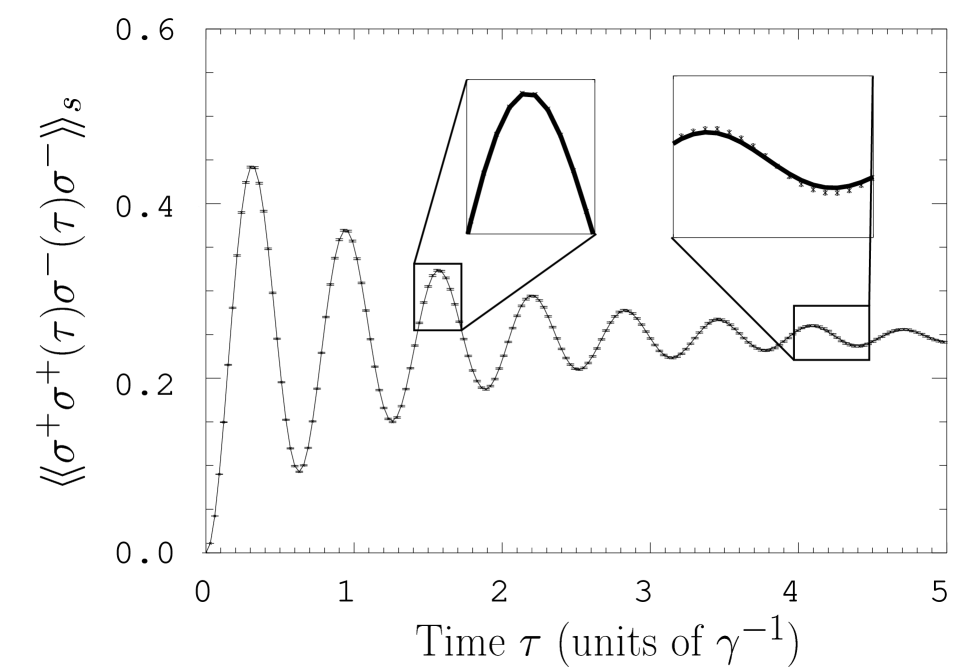
FIG. 1.: Correlation function $\langle\!\langle\sigma^{+}\sigma^{+}(\tau)\sigma^{-}(\tau)\sigma^{-}\rangle\!\rangle_{s}$ for a coherently driven two level atom on resonance with Rabi frequency $\Omega=10\gamma$. The numerical result for $10^{5}$ realizations of the simulation algorithm described in Sec. V A (errorbars) and analytical solution (thick line).

FIG. 2.: Calculation of the first order correlation function $\langle\!\langle\sigma^{+}(\tau)\sigma^{-}\rangle\!\rangle_{s}$ for a coherently driven two level atom on resonance. This figure shows the CPU time in seconds vs. the relative error for the simulation algorithms proposed in [1] (Method I) and for our algorithm (cf. Sec. V B 2, Method II). The solid lines represent the mean square deviation of the numerical solution from the exact solution and the dashed lines show the estimated standard deviation of the numerical solution.

FIG. 3.: Resonance fluorescence spectra for a coherently driven two level atom with Rabi frequency $\Omega=10\gamma$ coupled to a squeezed vacuum for different squeezing parameters (mean photon number $N$, relative phase of squeezing and driving field $\phi=2(\phi_{s}-\phi_{L})$, and fraction $\varepsilon$ of solid angle which is squeezed): numerical results (solid line), and the vacuum spectrum (thin line). The numerical solution was obtained by simulating a stochastic process in a doubled Hilbert space (cf. Sec. V B 2).

REFERENCES

- [1] J. Dalibard, Y. Castin, and K. Mølmer, Phys. Rev. Lett. 68, 580 (1992).
- [2] Carmichael, H., An Open Systems Approach to Quantum Optics, Lecture Notes in Physics m18 (Springer-Verlag, Berlin, Heidelberg, New York, 1993).
- [3] C. W. Gardiner, A. S. Parkins, and P. Zoller, Phys. Rev. A 46, 4363 (1992).
- [4] R. Dum, A. S. Parkins, P. Zoller, and C. W. Gardiner, Phys. Rev. A 46, 4382 (1992).
- [5] N. Gisin and I. C. Percival, J. Phys. A 25, 5677 (1992).
- [6] N. Gisin and I. C. Percival, J. Phys. A 26, 2233 (1993).
- [7] H. P. Breuer and F. Petruccione, Phys. Rev. E 51, 4041 (1995).
- [8] H. P. Breuer and F. Petruccione, Phys. Rev. Lett. 74, 3788 (1995); Phys. Rev. E 52, 428 (1995).
- [9] H. M. Wiseman and G. J. Milburn, Phys. Rev. A 47, 642 (1993).
- [10] H. M. Wiseman and G. J. Milburn, Phys. Rev. A 47, 1652 (1993).
- [11] H. P. Breuer and F. Petruccione, Phys. Rev. A 54, 1146 (1996).
- [12] H. P. Breuer and F. Petruccione, Fortschr. Phys. 45, 39 (1997).
- [13] K. Mølmer, Y. Castin, and J. Dalibard, J. Opt. Soc. Am. B 10, 524 (1993).
- [14] H. P. Breuer, W. Huber, and F. Petruccione, Stochastic Wave-Function Method versus Density Matrix: A Numerical comparison, Comput. Phys. Commun., in press.
- [15] A. S. Parkins, P. Zoller, and H. J. Carmichael, Phys. Rev. A 48, 758 (1993).
- [16] J. F. Poyatos, J. I. Cirac, and P. Zoller, Phys. Rev. Lett. 77, 4728 (1996).
- [17] L.-A. Wu, M. Xiao, and H. J. Kimble, J. Opt. Am. B 4, 1465 (1987).
- [18] D. F. Walls and G. J. Milburn, Quantum Optics (Springer-Verlag, Berlin, Heidelberg, New York, 1994).
- [19] C. W. Gardiner, Quantum Noise (Springer-Verlag, Berlin; Heidelberg, New York, 1991).
- [20] R. Alicki and K. Lendi, Lecture Notes in Physics: Quantum Dynamical Semigroups and Applications (Springer-Verlag, Berlin, Heidelberg, New York, 1987).
- [21] S. G. Sondermann, J. mod. Optics 42, 1659, (1995).
- [22] N. Gisin, J. mod. Optics 40, 2313 (1993).
- [23] L. P. Hughston, R. Jozsa, and W. K. Wootters, Phys. Lett. A 183, 14 (1993).
- [24] B. R. Mollow, Phys. Rev. A 12, 1919 (1975).
- [25] W. Feller, An Introduction to Probability Theory and its Applications (John Wiley & Sons, Inc, New York, London, Sydney, 1950), Vol. 2.
- [26] M. H. A. Davis, Markov Models and Optimization (Chapman & Hall, London, 1993).
- [27] H. P. Breuer and F. Petruccione, J. Phys. A 29, 7837 (1996).
- [28] R. Hanbury-Brown and R. Q. Twiss, Nature 177, 27 (1956).
- [29] F. Diedrich and H. Walther, Phys. Rev. Lett. 58, 203 (1987).
- [30] C. W. Gardiner and M. J. Collett, Phys. Rev. A 31, 3761 (1985).
- [31] B. R. Mollow, Phys. Rev. 188, 1969 (1969).
- [32] H. J. Carmichael, A. S. Lane, and D. F. Walls, Phys. Rev. Lett. 58, 2539 (1987).