Measuring quantum optical Hamiltonians

Abstract

We show how recent state-reconstruction techniques can be used to determine the Hamiltonian of an optical device that evolves the quantum state of radiation. A simple experimental setup is proposed for measuring the Liouvillian of phase-insensitive devices. The feasibility of the method with current technology is demonstrated on the basis of Monte Carlo simulated experiments.

PACS: 03.65.Bz, 42.55.-f

In recent years, the possibility of “measuring” the quantum state, after remaining for a longtime a mere theoretical speculation [1], eventually entered the realm of true experiments. From the first experimental demonstration [2], the so called “homodyne tomography” technique advanced to the level of a quantitative state-reconstruction technique [3, 4], achieving a high degree of reliability in experiments [5]. This state-reconstruction method is now ready to be used for concrete applications.

What is the practical use of measuring a quantum state? Apart from the availability of a kind of “universal detector” [6] that provides informations on all observables at a time, measuring a quantum state is the only way to check a state preparation within a (generally nonorthogonal) set. In turn, the use of homodyne tomography to test state-preparation becomes a way to check the operation of a quantum device that prepares a chosen state from a given one. It is now natural to ask if eventually it would be possible to recover a complete information on the quantum device itself, namely to reconstruct the detailed form of its Hamiltonian— or, more generally, of its Liouvillian, as in reality the device is always an open quantum system. Previous theoretical proposals to give a complete characterization of quantum processes have been made in Refs. [7, 8]. There, the methods are restricted to systems with finite dimensional Hilbert space, and the method does not lead to an explicit reconstruction of the Liouvillian. In this letter we show how this goal can be achieved in practice, presenting a simple experimental setup for measuring the Liouvillian of a phase-insensitive optical device, using currently available technology.

The main idea for reconstructing the Liouvillian of a quantum device is sketched in Fig. 1. One should impinge the device with a known input state $\rho_{in}$ from a (over)complete set, then determine the state $\rho_{out}$ at the output, and finally compare $\rho_{in}$ to $\rho_{out}$. For an optical device the determination of the output state is made possible by the homodyne-tomography technique. Regarding the generation of the set of input states $\{\rho_{in}\}$, an experimental method is suggested later in this letter. The evolution of the state from $\rho_{in}$ to $\rho_{out}$ is governed by the Green (super)operator $\cal G$

$$\rho_{out}={\cal G}\rho_{in}\;,$$ (1)

where $\cal G$ has actually a four-index matrix representation, and on the Fock basis one has $\langle n|\rho_{out}|m\rangle=\sum_{h,k=0}^{\infty}\ {G}^{hk}_{nm}\langle h|\rho_{in}|k\rangle$.

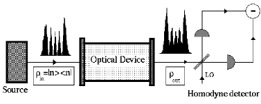
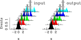
FIG. 1.: Sketch of the method for measuring the Liouvillian of an optical device. A known input state $\rho_{in}$ is impinged into the device, and a quantum tomography of the output state is performed using a homodyne detector. By scanning an (over)complete set of states $\rho_{in}$ at the input and comparing them with their respective output states, it is possible to reconstruct the Liouvillian of the device. The histograms of homodyne data, here given for the sake of illustration, correspond to a device that consists of an empty cavity, and with the input states as number states $\rho_{in}=|n\rangle\langle n|$.

For a device that is homogeneous along the direction of light propagation the Green superoperator can be written as the exponential of a constant Liouville superoperator $\cal L$ as follows

$${\cal G}=\exp({\cal L}\tau)\;,$$ (2)

where $\tau$ is the propagation time (i.e. the device length). The Liouvillian $\cal L$ gives the evolution of the state through an infinitesimal slab of the device media according to the master equation $\dot{\rho}={\cal L}\rho$. In this letter we restrict our attention to the case of a perfectly phase-insensitive device: as it will be clear from the following, the case of phase-sensitive device is much more complicate, and will be analyzed elsewhere [9]. A phase-insensitive device, is a device that leaves dephased states as dephased, as in the case of a traveling wave laser amplifier. A dephased state is diagonal in the photon-number representation, with density matrix of the form $\rho=\sum_{n=0}^{\infty}\ r_{n}\ |n\rangle\langle n|$, where $\{|n\rangle\}$ denotes the complete set of eigenvectors of the photon-number operator $a^{\dagger}a$ of the field mode with annihilation operator $a$. For the evolution of dephased states it is sufficient to determine the sector of the Green superoperator that evolves dephased states, i.e. the two-index Fock matrix $G_{nm}=\langle n|\,\,{\cal G}[\,|m\rangle\langle m|\,]\,\,|n\rangle$.

The experimental reconstruction of $L_{nm}$ could be performed by impinging a number state $\rho_{in}=|n\rangle\langle n|$ on the device, and then making the homodyne tomography of the output state. In this fashion, the number probability distribution $r_{k}(n)$ of the output coincides with the $n$-th row of the Green matrix $G_{nm}$, and by varying $n$ one would reconstruct the whole matrix. Since producing number states is experimentally difficult, one would try to use coherent states instead. In this way matrix elements of the form $\langle\psi|\,\,{\cal G}[\,|\alpha\rangle\langle\alpha|\,]\,\,|\psi^{\prime}\rangle$ would be obtained, with $|\alpha\rangle$ denoting the scanning coherent input state, and $|\psi\rangle$ and $|\psi^{\prime}\rangle$ being a couple of vectors of the tomographically reconstructed matrix representation. Unfortunately, the relation between $G_{nm}$ and $\langle n|\,\,{\cal G}[\,|\alpha\rangle\langle\alpha|\,]\,\,|n\rangle$ is highly singular, involving the $P$-function of $|m\rangle\langle m|$, and hence the matrix $G_{nm}$ cannot be obtained in this way starting from experimental data. On the other hand, the Fock representation has a privileged role, because here the Liouvillian matrix has a transparent meaning in terms of creation and annihilation operators. How to overcome the problem of generating input number-states? Actually, for our purpose, it is sufficient to generate number states with random $n$ as far as $n$ is known. This leads us to devise the setup depicted in Fig. 2.

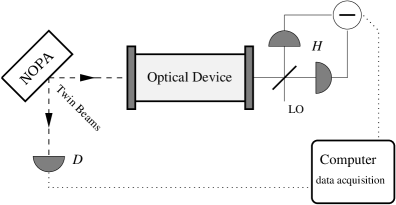
FIG. 2.: Experimental setup, including the apparatus used to generate the input number states $\rho_{in}=|n\rangle\langle n|$ needed for the tomographical reconstruction of the Liouvillian of an optical device. A random-$n$ Fock state $|n\rangle$ for the input beam is achieved by performing photodetection at $D$ on the other twin beam, $n$ being the measured number of photons. A non degenerate optical parametric amplifier (NOPA) with vacuum input is used to produce the twin beams.

A non degenerate optical parametric amplifier (NOPA) with a strong classical pump down-converts the vacuum into a pair of twin beams. The twin beams are used as a random-$n$ Fock state generator, by measuring the number of photons on one beam (detector $D$ in Fig. 2) while impinging the other beam on the optical device. For quantum efficiency $\eta_{D}=1$ at detector $D$, the photodetection would reduce the twin-beam state $|\mbox{TB}\rangle\propto\sum^{\infty}_{n=0}\kappa^{n}|n,n\rangle$ into a random-$n$ state $|n\rangle$ at the input of the optical device, with thermal probability distribution $w_{n}=|\kappa|^{2n}\left(1-|\kappa|^{2}\right)$, where $n$ is the measurement outcome at $D$. The tomographically reconstructed number probability $\langle k|\,\,{\cal G}[\,|n\rangle\langle n|\,]\,\,|k\rangle$ of the output state already would provide the $n$th row $G_{kn}$ of the Green matrix. On the other hand, for $\eta_{D}<1$, a mixed state $\rho_{n}$ will actually enter the device instead of $|n\rangle\langle n|$, as a result of state reduction at $D$. The outcome $n$ probability distribution then becomes

$$p_{n}=(1-|\kappa|^{2})\frac{(\eta_{D}|\kappa|^{2})^{n}}{[(\eta_{D}-1)|\kappa|^{2}+1]^{n+1}}\;.$$ (3)

One can easily show that the tomographically reconstructed output number probability $r_{k}(n)\equiv\langle k|{\cal G}[\rho_{n}]|k\rangle$ is related to the Green matrix through the identity

$$r_{k}(n) = [(\eta_{D}-1)|\kappa|^{2}+1]^{n+1}$$ (4)

$$\times \sum_{m=0}^{\infty}{m+n\choose n}[|\kappa|^{2}(1-\eta_{D})]^{m}G_{k,m+n}\;.$$ (5)

The relation (5) can be inverted as follows

$$G_{kl} = \frac{1}{[(\eta_{D}-1)|\kappa|^{2}+1]^{l+1}}$$ (6)

$$\times \sum_{n=0}^{\infty}{n+l\choose l}\left[\frac{(\eta_{D}-1)|\kappa|^{2}}{(\eta_{D}-1)|\kappa|^{2}+1}\right]^{n}r_{k}(n+l)\;.$$ (7)

Eq. (7) is our algorithm to reconstruct the Green matrix $G_{kl}$ from the collection of all tomographically measured number probabilities $r_{k}(n)$ for different outcomes $n$ (in practice the sum in Eq. (7) is truncated at some maximum $n$). Notice the interplay of the gain $\kappa$ and the quantum efficiency $\eta_{D}$ in determining the probability $p_{n}$ on one hand, and in producing the statistical errors in the reconstructed Green matrix on the other hand. For decreasing quantum efficiency $\eta_{D}\to 0$, larger values of $n$ can be made more probable by increasing the gain of the NOPA as $\kappa\to 1^{-}$. However, at the same time, convergence of the sum in Eq. (7) becomes slower, and statistical errors of matrix elements $G_{kl}$ increase as result of tomographic errors on $r_{k}(n)$. Hence, the effect of quantum efficiency $\eta_{D}$, which reduces the size of the viewable matrix $G_{kl}$, can be partially compensated by increasing the gain of the NOPA, however at expense of statistical errors for $G_{kl}$. For the tomographic measurement, by increasing the number of experimental data and using $\eta_{H}$-dependent pattern functions, the method of Ref. [4] can compensate the effect of low quantum efficiency $\eta_{H}<1$, that, anyhow, must be above the threshold $\eta_{H}=1/2$. On the other hand, for quantum efficiency $\eta_{D}$ at detector $D$ there is not such a threshold, as one can see from convergence and and error-propagation analysis of Eq. (7).

The proposed state-reduction scheme—based on twin-beams from a NOPA—is not a new one, and, for example, a similar setup has been proposed in Ref.[10] to generate Schrödinger-cat states. As such state-reduction is the core of our measurement method, we want to examine it at work in a realistic situation. Typically the NOPA can be pumped by the second harmonic of a Q-switched mode-locked Nd:YAG laser, with the output twin-beams pulsed at a repetition rate of 80 MHz, and with a 7ps pulse duration. Thus, the twin-beam mode with annihilator $a$ at the input of the optical device is actually a wideband mode, with frequency centered around 532nm, and width of 140 GHz (the inverse of the pulse time-length). The same Nd:YAG laser beam is used for the local oscillator (LO) of the homodyne detector $H$. In this way the LO has the same central frequency and the same time-envelope of the beam at the input of the optical device. The integration time at photodetector $D$ can be set to 1 ns, which is greater than the pulse width and shorter than the distance between pulses. In this way each pulse is completely annihilated by the detector $D$ during the integration time, and, correspondingly, the homodyne measurement is made with the LO matched on the same pulse shape of the signal twin-beam, which means that the measurement is performed on the right wideband mode after reduction by detector $D$. Moreover, the detector $D$ and the optical device can be geometrically placed in such a way that, within a narrow solid angle, the direction of the respective input $k$-vectors are the same relative to the $k$-vector of the NOPA pump, so that state reduction at $D$ affects only radiation at the twin $k$ at the input of the device, so that the state-reduced modes at $D$ and at the device are perfectly matched.

From the above scenario it follows that the mode with annihilator $a$ at the input of the optical device is actually a wideband mode, and hence we measure the effective Liouvillian over a 140 GHz bandwidth centered around 532nm. Then, it is clear that all measurements for different random inputs can be considered as independent only if the (atomic) relaxation times in the optical devices are shorter than the pulse-repetition period.

Now we show results from some Monte-Carlo simulated experiments to see our method at work, and estimate the number of measurements needed for the reconstruction of $G_{kl}$.

The simplest phase insensitive device is the phase-insensitive linear amplifier (PIA), with Liouvillian $\cal L$

$${\cal L}=2\left\{A{\cal D}[a^{\dagger}]+B{\cal D}[a]\right\}\;,$$ (8)

where ${\cal D}[\theta]\rho\doteq\theta\rho\theta^{\dagger}-1/2(\theta^{\dagger}\theta\rho+\rho\theta^{\dagger}\theta)$ for any complex operator $\theta$. The Liouvillian matrix has the form

$$L_{nm}\doteq\langle n|{\cal L}\Big{[}|m\rangle\langle m|\Big{]}|n\rangle=$$ (9)

$$2\Big{\{}A(m+1)[\delta_{nm+1}-\delta_{nm}]+Bm[\delta_{nm-1}-\delta_{nm}]\Big{\}} \;,$$ (10)

where $\delta_{ik}$ denotes the Kroneker delta. Notice that $L_{nm}$ is tridiagonal, the upper diagonal corresponding to the one-photon absorption $a\rho a^{\dagger}$ of the loss term ${\cal D}[a]$, the lower diagonal corresponding to the one-photon emission $a^{\dagger}\rho a$ of the gain term ${\cal D}[a^{\dagger}]$, and the main diagonal containing the anticommutators coming from both terms.

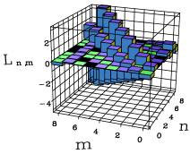
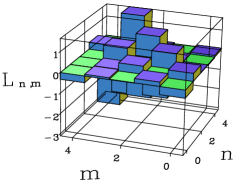
(a)                              (b)

FIG. 3.: (a) Linear phase insensitive laser amplifier with $A=.1940$ and $B=.00945$. Monte Carlo simulation of the reconstruction of the Liouvillian $L_{nm}$ in Eq. 9 by means of the proposed experimental setup. The reconstruction is performed by using 2 statistical blocks of $10^{6}$ homodyne data for each of the output states (from a total of $2.7*10^{11}$ of data). Quantum efficiencies are $\eta_{D}=.8$ and $\eta_{H}=.85$. The gain of the NOPA is $\kappa=.6$. (b) the same reconstruction for lower quantum efficiency $\eta_{D}=.3$. Here the gain is set to $\kappa=.4$, and the same number of data is used out of a total of $9.9*10^{11}$.

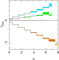
FIG. 4.: The three main diagonals of the Liouvillian $L_{nm}$ of Fig. 3a are given with their statistical error bars. The full line is the theoretical value from Eq. (9).

In Fig 3a we show a typical result of a Monte Carlo experiment of the tomographic reconstruction of the Liouvillian (9). We used quantum efficiency $\eta_{D}=.8$ and $\eta_{D}=.3$ at detector $D$ and $\eta_{H}=.85$ at the homodyne detector $H$. One can see that the details of the matrix are well recovered, and the truncation of the Hilbert space dimension does not affect the reconstruction. In Fig. 4 the three main diagonals of the matrix are plotted with their statistical errors against the theoretical value, showing a very good agreement. The statistical errors are of the same size of those of the tomographically reconstructed output probabilities. Notice that the number of data $10^{11}\div 10^{12}$ needed for this experiment could be collected in a few minutes at the repetition rate of 80 MHz. In Fig. 3b we present a simulated experiment using the very realistic value $\eta_{D}=.3$ of quantum efficiency, however for the reconstruction of a smaller matrix $5\times 5$. Notice that only the photodetector $D$ is required to be linear single-photon resolving, whereas the homodyne detector takes advantage of amplification from the LO, and hence can use high efficiency detectors (the value $\eta_{H}=.85$ here used has been widely surpassed in the real tomographic experiments, as in Ref. [5]).

As another example, we simulated the experimental tomography of the effective Liouvillian of a one-atom traveling-wave laser amplifier.

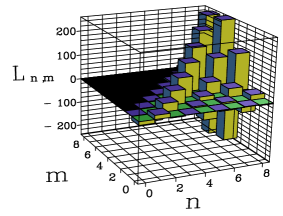
FIG. 5.: Theoretical Liouvillian for a one-atom laser, obtained by solving numerically the master equation (12). The parameters for this laser are $C\doteq\frac{g^{2}}{\gamma\gamma_{\perp}}=12$; $n_{s}\doteq\frac{\gamma_{\parallel}\gamma_{\perp}}{4g^{2}}=7$; $\sigma_{0}=1;\;f=\frac{\gamma_{\parallel}}{2\gamma_{\perp}}=1$; $\gamma=1$; $t_{*}=.0115$.

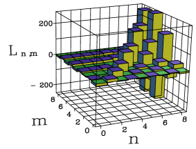
FIG. 6.: Monte Carlo simulated experiment for the reconstruction of the laser theoretical Liouvillian in Fig. 5. Here $\eta_{D}=.8$, $\eta_{H}=.85$, and $\kappa=.65$. A set of $8*10^{7}$ homodyne data have been used of a total of $3.7*10^{11}$ measurements with random photon number at detector $D$.

In Fig. 5 the theoretical Liouvillian matrix is plotted, as obtained from a long-run quantum jump simulation of the one-atom-laser master equation [11]:

$$\dot{\rho}=\bigg{\{}\frac{\gamma_{\|}}{2}(1+\sigma_{0}){\cal D}[\sigma_{+}]+\frac{\gamma_{\|}}{2}(1-\sigma_{0}){\cal D}[\sigma_{-}]+$$ (11)

$$\frac{1}{4}\left(\gamma_{\perp}-\frac{\gamma_{\|}}{2}\right){\cal D}[\sigma_{z}]+\gamma{\cal D}[a]\bigg{\}}\rho+g[\sigma_{+}a-\sigma_{-}a^{\dagger},\rho]$$ (12)

where $g$ is the electrical-dipole coupling, $\gamma_{\|}$ and $\gamma_{\perp}$ are the decay rates of population inversion and atomic polarization respectively, $\gamma$ is the cavity decay rate, $\sigma_{0}$ is the unsaturated inversion ($-1\leq\sigma_{0}\leq 1$), $\sigma_{\pm z}$ are the Pauli matrices (with $0,\pm 1$ entries), and $\rho$ now denotes the joint atom-radiation density matrix. In the quantum jump simulation, the atom is traced out at a time $t_{*}\gg\gamma^{-1}_{\|,\perp}$. In Fig. 6 a Monte Carlo simulated tomographic experiment is shown for reconstructing the Liouvillian in Fig. 5 (the output homodyne probabilities are simulated starting from the quantum jump Green matrix). One can see how the method allows a detailed reconstruction of $L_{nm}$, including not only one-photon processes on the three main diagonals, but also multiphoton-absorptions on the upper triangular part.

In conclusion, we have seen that it is possible to experimentally reconstruct the Liouvillian of a quantum optical phase-insensitive device, using homodyne tomography in a scheme based on parametric down conversion from a NOPA. We have shown the feasibility of the reconstruction with an experimental setup that uses standard technology devices. The problem of low efficiency at the single-photon resolving detector $D$—the major obstacle for the experiment—has been solved by implementing a compensation algorithm that makes the reconstruction of $5\times 5$ Liouville matrix possible even for $\eta_{D}=.3$, and with a number of data that can be collected in a few minutes of experimental run.

REFERENCES

- [1] U. Fano, Rev. Mod. Phys. 29, 74 (1957); B. d’Espagnat, Conceptual Foundations of Quantum Mechanics, W. A. Benjamin, Massachusetts (1976)
- [2] D. T. Smithey, M. Beck, M. G. Raymer and A. Faridani, Phys. Rev. Lett. 70,1244 (1993)
- [3] G. M. D’Ariano, C. Macchiavello, M. G. A. Paris, Phys. Rev. A 50, 4298 (1994)
- [4] G. M. D’Ariano, U. Leonhardt, M. Paul, Phys. Rev. A 52 R1801 (1995)
- [5] G. Breitenbach, S. Schiller and J. Mlynek, Nature 387, 471 (1997).
- [6] G. M. D’Ariano, in “Quantum Communication, Computing and Measurement”, ed. by O. Hirota, A. S. Holevo, and C. M. Caves (Plenum Publishing New York and London 1997), p. 253.
- [7] J. F. Poyatos, J. I. Cirac, and P. Zoller, Phys. Rev. Lett. 78 390 (1997)
- [8] I. L. Chuang and M. A. Nielsen, J. Mod. Opt. 44 2455 (1997)
- [9] G. M. D’Ariano, L. Maccone unpublished.
- [10] S. Song, C. M. Caves, B. Yurke, Phys. Rev. A 41 5261 (1990)
- [11] C. Ginzel, M. J. Brigel, U. Martini, B. G. Englert, A. Schenzle, Phys. Rev. A 48, 732 (1993)