Sonoluminescence as a QED vacuum effect: Probing Schwinger’s proposal

Abstract

Several years ago Schwinger proposed a physical mechanism for sonoluminescence in terms of photon production due to changes in the properties of the quantum-electrodynamic (QED) vacuum arising from a collapsing dielectric bubble. This mechanism can be re-phrased in terms of the Casimir effect and has recently been the subject of considerable controversy. The present paper probes Schwinger’s suggestion in detail: Using the sudden approximation we calculate Bogolubov coefficients relating the QED vacuum in the presence of the expanded bubble to that in the presence of the collapsed bubble. In this way we derive an estimate for the spectrum and total energy emitted. We verify that in the sudden approximation there is an efficient production of photons, and further that the main contribution to this dynamic Casimir effect comes from a volume term, as per Schwinger’s original calculation. However, we also demonstrate that the timescales required to implement Schwinger’s original suggestion are not physically relevant to sonoluminescence. Although Schwinger was correct in his assertion that changes in the zero-point energy lead to photon production, nevertheless his original model is not appropriate for sonoluminescence. In other work we have developed a variant of Schwinger’s model that is compatible with the physically required timescales.

PACS:12.20.Ds; 77.22.Ch; 78.60.Mq

I Introduction

In this paper we shall concentrate on Schwinger’s original proposal regarding sonoluminescence [5, 6, 7, 8, 9, 10, 11], that of photon production associated with changes in the QED vacuum state. His idea was to explain the sonoluminescence phenomenon, which consists in light emission by a sound-driven gas bubble in fluid [12], in the framework of the so-called dynamical Casimir effect. Our first aim is to verify, in a dynamic framework, that a sudden change in bubble size will cause efficient photon production, thereby indicating the possibility of an a priori interesting role for the dynamic Casimir effect in this condensed matter context. While we demonstrate that the key features of Schwinger’s calculations are correct, this study also demonstrates that for other reasons (to do with the observed timescale of the phenomenon) the original approach of Schwinger is not physically relevant to sonoluminescence. In related work [13, 14, 15, 16] we have developed a different implementation of Schwinger’s ideas regarding sonoluminescence that is compatible with the physically observed timescales.

The idea of a “Casimir route” to sonoluminescence was developed by Schwinger in a series of papers [5, 6, 7, 8, 9, 10, 11]. One key issue in Schwinger’s model is simply that of calculating static Casimir energies for dielectric spheres—and there is already considerable disagreement on this issue. A second and in some ways more critical question is the extent to which a change in static Casimir energies might be converted to real photons during the collapse of the bubble—it is this issue that we shall address in this paper. We estimate the spectrum of the emitted photons by calculating an appropriate Bogolubov coefficient relating the two states of the QED vacuum.

Another model associating sonoluminescence with QED vacuum changes is the variant of Schwinger’s proposal due to Eberlein [17, 18, 19]. In contrast to Schwinger’s quasi-static approach, Eberlein’s model is truly dynamical but uses a radically different physical approximation—the adiabatic approximation. The two models should not be confused. See [14] for a deeper discussion of Eberlein’s approach to sonoluminescence.

Considerable confusion has been caused by Schwinger’s choice of the phrase “dynamical Casimir effect” to describe his model. In fact, the original model is not dynamical and is better described as quasi-static as the heart of the model lies in comparing two static Casimir energy calculations: that for an expanded bubble with that for a collapsed bubble. In a series of papers [5, 6, 7, 8, 9, 10, 11] Schwinger showed that the dominant bulk contribution to the Casimir energy of a bubble (of dielectric constant $\epsilon_{inside}$) in a dielectric background (of dielectric constant $\epsilon_{outside}$) is

$$E_{cavity} = +2\frac{4\pi}{3}R^{3}\;\int_{0}^{K}{4\pi k^{2}dk\over(2\pi)^{3}}\;\frac{1}{2}\hbar ck\left({1\over\sqrt{\epsilon_{inside}}}-{1\over\sqrt{\epsilon_{outside}}}\right)+\cdots$$ (1)

$$= +\frac{1}{6\pi}\hbar cR^{3}K^{4}\left({1\over\sqrt{\epsilon_{inside}}}-{1\over\sqrt{\epsilon_{outside}}}\right)+\cdots.$$ (2)

There are additional sub-dominant finite volume effects [20, 21, 22]. The quantity $K$ is a high-wavenumber cutoff that characterizes the wavenumber at which the dielectric constants drop to their vacuum values. This result can also be rephrased in the clearer and more general form as [20, 21, 22]:

$$E_{cavity}=+2V\int\frac{d^{3}\vec{k}}{(2\pi)^{3}}\;\frac{1}{2}\hbar\left[\omega_{inside}(k)-\omega_{outside}(k)\right]+\cdots$$ (3)

where it is evident that the Casimir energy can be interpreted as a difference in zero point energies due to the different dispersion relations inside and outside the bubble.

In contrast, Milton [23], and Milton and Ng [24, 25] strongly criticize Schwinger’s result. Using what is to our minds a physically dubious renormalization argument leads them [25] to discard both the volume and even the surface term and to claim that the Casimir energy for any dielectric bubble is of order $E\approx\hbar c/R$.

In [20, 21, 22] an extensive discussion on these topics is found. Therein it is emphasized that one has to compare two different geometrical configurations, and different quantum states, of the same spacetime regions. In a situation like that of Schwinger’s model one has to subtract from the zero point energy (ZPE) for a vacuum bubble in water the ZPE for water filling all space. It is clear that in this case the bulk term is physical and must be taken into account. In the situation pertinent to sonoluminescence, the total volume occupied by the gas is not constant (the gas is truly compressed), and it is far too naive to simply view the ingoing water as flowing coherently from infinity (leaving voids filled with air or vacuum somewhere in the apparatus). Since the density of water is approximately but not exactly constant, the influx of water will instead generate an outgoing density wave which will be rapidly damped by the viscosity of the fluid. The few phonons generated in this way are surely negligible. Surface terms are also present, and eventually other higher order correction terms, but they prove to not be dominant for sufficiently large cavities [22].

II Bogolubov coefficients

As a first approach to the problem we study in detail the basic mechanism of particle creation, and test the consistency of the Casimir energy proposals previously described. With this aim in mind we consider the change in the QED vacuum associated with the collapse of the bubble, by keeping fixed the refractive index both of the gas and of the water. For the sake of simplicity we take, as Schwinger did, only the electric part of QED, reducing the problem to a scalar electrodynamics. Moreover, at this stage of development, we are not concerned with the dynamics of the bubble surface. In analogy with the subtraction procedure of the quasi-static calculations of Schwinger [5, 6, 7, 8, 9, 10, 11], and of Carlson et al. [20, 21, 22], we shall consider two different configurations of space. An “in” configuration with a bubble of dielectric constant $\epsilon_{inside}$ (typically vacuum) in a medium of dielectric constant $\epsilon_{outside}$, and an “out” one in which one has just the latter medium (dielectric constant $\epsilon_{outside}$) filling all space. Strictly speaking we should compare a large bubble having radius $R_{\mathrm{m}ax}$ with a small bubble of radius $R_{\mathrm{m}in}$. We are approximating the small bubble by zero volume on the grounds that the small bubble that is relevant to sonoluminescence is at least a million times smaller than the large bubble at the expansion maximum. Keeping $R_{\mathrm{m}in}$ finite significantly complicates the calculation but does not give much more physical information. The above “in” and “out” configurations will correspond to two different bases for the quantization of the field. The two bases will be related by Bogolubov coefficients in the usual way. Once we determine these coefficients we easily get the number of created particles per mode and from this the spectrum. This tacitly makes the “sudden approximation”: Changes in the refractive index are assumed to be non-adiabatic, see [13, 14, 15] for more discussion. We shall also make a consistency check by a direct confrontation between the change in Casimir energy and the direct sum, $E=\sum_{k}\omega_{k}n_{k}$ of the energies of the created photons. The former energy (the total energy of the particles that can be produced by the collapse) must necessarily equal the Casimir energy of the bubble in the “in” state since in the current simplified model there is no external source of energy (like the driving sound in the true dynamical effect). For this reason we expect to be able to give a definitive answer on the nature (dependence on the bubble radius and on the cut-off) of the static Casimir energy. Of course it is evident that such a model cannot be considered a fully satisfactory model for sonoluminescence. In fact this model completely ignores the details of the dynamics and moreover, by considering just one cycle, implies impossibility of testing for the possible presence of any parametric resonances. We thus consider the present calculation as a toy model in which some basic features of the Casimir approach to sonoluminescence are investigated: it provides a test of the nature and quantity of the particles produced by a collapsing dielectric bubble in the sudden approximation.

A Formal calculation

Let us consider the equations of the electric fields (Schwinger framework) in spherical coordinates and with a time independent dielectric constant (we temporarily set $c=1$ for ease of notation, and shall reintroduce appropriate factors of the speed of light when needed for clarity)

$$\epsilon\partial_{0}(\partial_{0}E)-\nabla^{2}E=0.$$ (4)

We look for solutions of the form

$$E=\Phi(r,t)Y_{lm}(\Omega){1\over r}.$$ (5)

Then one finds

$$\epsilon(\partial^{2}_{0}\Phi)-(\partial_{r}^{2}\Phi)+{1\over r^{2}}l(l+1)\Phi=0.$$ (6)

For both the “in” and “out” solution the field equation in $r$ is given by:

$$\epsilon\partial_{0}^{2}\Phi-\partial_{r}^{2}\Phi+{1\over r^{2}}l(l+1)\Phi=0.$$ (7)

In both asymptotic regimes (past and future) one has a static situation (either a bubble in the dielectric, or just the dielectric) so one can in this limit factorize the time and radius dependence of the modes: $\Phi(r,t)=e^{i\omega t}f(r)$. One gets

$$f^{{}^{\prime\prime}}+\left(\epsilon\omega^{2}-{1\over r^{2}}l(l+1)\right)f=0.$$ (8)

This is a well known differential equation. To handle it more easily in a standard way we can cast it as an eigenvalues problem

$$f^{{}^{\prime\prime}}-\left({1\over r^{2}}l(l+1)\right)f=-\lambda^{2}f,$$ (9)

where $\lambda^{2}=\epsilon\omega^{2}$. With the change of variables $f=r^{1/2}G$ we get

$$G^{{}^{\prime\prime}}+{1\over r}G^{{}^{\prime}}+\left(\lambda^{2}-{\nu^{2}\over r^{2}}\right)G=0.$$ (10)

This is the standard Bessel equation. It admits as solutions the first type Bessel and Neumann functions, $J_{\nu}(\lambda r)$ and $N_{\nu}(\lambda r)$, with $\nu=l+1/2$. Remember that for those solutions which have to be well-defined at the origin, $r=0$, regularity implies the absence of the Neumann functions. For the “in” basis we have to take into account that the dielectric constant changes at the bubble radius ($R$). In fact we have

$$\epsilon=\left\{\begin{array}[]{llllll}\epsilon_{inside}&=&n^{2}_{gas}&=&\mbox{dielectric constant of air-gas mixture}&\mbox{if $r\leq R$},\\ \epsilon_{outside}&=&n^{2}_{liquid}&=&\mbox{dielectric constant of ambient liquid (typically water)}&\mbox{if $r>R$}.\end{array}\right.$$ (11)

Typically one simplifies calculations by using the fact that the dielectric constant of air is approximately equal 1 at standard temperature and pressure (STP), and then dealing only with the dielectric constant of water ($n_{liquid}=\sqrt{\epsilon_{outside}}\approx 1.3$). We find it convenient to explicitly keep track of $n_{gas}$ and $n_{liquid}$ in the formalism we develop. Defining the in and out frequencies, $\omega_{in}$ and $\omega_{out}$ respectively, one has

$$G^{in}_{\nu}(n_{gas},n_{liquid},\omega_{in},r)=\left\{\begin{array}[]{ll}A_{\nu}J_{\nu}(n_{gas}\,\omega_{in}r)&\mbox{if $r\leq R$},\\ B_{\nu}J_{\nu}(n_{liquid}\,\omega_{in}r)+C_{\nu}N_{\nu}(n_{liquid}\,\omega_{in}r)&\mbox{if $r>R$.}\end{array}\right.$$ (12)

The $A_{\nu}$, $B_{\nu}$, and $C_{\nu}$ coefficients are determined by matching conditions in $R$

$$\begin{array}[]{lll}A_{\nu}J_{\nu}(n_{gas}\,\omega_{in}R)&=&B_{\nu}J_{\nu}(n_{liquid}\,\omega_{in}R)+C_{\nu}N_{\nu}(n_{liquid}\,\omega_{in}R),\\ A_{\nu}J_{\nu}{{}^{\prime}}(n_{gas}\,\omega_{in}R)&=&B_{\nu}J_{\nu}{{}^{\prime}}(n_{liquid}\,\omega_{in}R)+C_{\nu}N_{\nu}{{}^{\prime}}(n_{liquid}\,\omega_{in}R).\end{array}$$ (13)

The “out” basis is easily obtained solving the same equation but for a space filled with a homogeneous dielectric,

$$G^{out}_{\nu}(n_{liquid},\omega_{out},r)=J_{\nu}(n_{liquid}\,\omega_{out}r).$$ (14)

To check that the “out” basis is properly normalized we use the scalar product, defined as usual by

$$(\phi_{1},\phi_{2})=-i\int_{\Sigma}\phi_{1}\stackrel{{\scriptstyle\leftrightarrow}}{{\partial}}_{0}\phi_{2}^{*}\>d^{3}x.$$ (15)

There are subtleties in the definition of scalar product which are dealt with more fully in [13, 14, 15]. The naive scalar product adopted here is missing a dependence on the refractive indices of the gas and the surrounding water. Given the fact that in the present framework both of these are approximately equal to one, the product adopted here is good enough for a qualitative discussion. Consider now the scalar product of a eigenfunction with itself, one expects to obtain a normalization condition which can be written as

$$((\Phi^{i}_{out})^{*},(\Phi^{j}_{out})^{*})=\delta^{ij}.$$ (16)

Inserting the explicit form of the $\Phi$ functions we get

$$((\Phi^{i}_{out})^{*},(\Phi^{j}_{out})^{*}) = (\lambda+\lambda^{\prime})\int_{0}^{\infty}rdrJ_{\nu}(\lambda r)J_{\nu}(\lambda^{\prime}r)e^{i(\lambda-\lambda^{\prime})}$$ (17)

$$= (\lambda+\lambda^{\prime})\frac{\delta(\lambda-\lambda^{\prime})}{\lambda}e^{i(\lambda-\lambda^{\prime})},$$ (18)

where we have used the Hankel Integral Formula [26]

$$\int_{0}^{\infty}rdrJ_{\nu}(\lambda r)J_{\nu}(\lambda^{\prime}r)=\delta(\lambda-\lambda^{\prime})/\lambda.$$ (19)

The Bogolubov coefficients are defined as

$$\alpha_{ij} = -({E_{i}^{out}}^{*},{E_{j}^{in}}^{*}),$$ (20)

$$\beta_{ij} = +(E_{i}^{out},{E_{j}^{in}}^{*}).$$ (21)

We are mainly interested in the coefficient $\beta$, since $|\beta|^{2}$ is linked to the total number of particles created. By a direct substitution it is easy to find the expression:

$$\beta = -i\int_{0}^{\infty}\left(\Phi_{out}(r,t)\;Y_{lm}(\Omega)\;{1\over r}\right)\stackrel{{\scriptstyle\leftrightarrow}}{{\partial}}_{0}\left(\Phi_{in}(r,t)\;Y_{l^{\prime}m^{\prime}}(\Omega)\;{1\over r}\right)^{*}\>r^{2}drd\Omega,$$ (22)

$$= (\omega_{in}-\omega_{out})\;e^{i(\omega_{out}+\omega_{in})t}\delta_{ll^{\prime}}\;\delta_{mm^{\prime}}\;\int_{0}^{\infty}G^{out}_{l}(n_{liquid},\omega_{out},r)\;G^{in}_{l^{\prime}}(n_{gas},n_{liquid},\omega_{in},r)\>rdr.$$ (23)

To compute the integral one needs some ingenuity. Let us write the equations of motion for two different values of the eigenvalues, $\lambda$ and $\mu$:

$$G_{\lambda}^{{}^{\prime\prime}}+{1\over r}G_{\lambda}^{{}^{\prime}}+\left(\lambda^{2}-{1\over r^{2}}(l+{1\over 2})^{2}\right)G_{\lambda} = 0,$$ (24)

$$G_{\mu}^{{}^{\prime\prime}}+{1\over r}G_{\mu}^{{}^{\prime}}+\left(\mu^{2}-{1\over r^{2}}(l+{1\over 2})^{2}\right)G_{\mu} = 0.$$ (25)

If we multiply the first by $G_{\mu}$ and the second by $G_{\lambda}$ we get

$$G_{\lambda}^{{}^{\prime\prime}}G_{\mu}+{1\over r}G_{\lambda}^{{}^{\prime}}G_{\mu}+\left(\lambda^{2}-{1\over r^{2}}(l+{1\over 2})^{2}\right)G_{\lambda}G_{\mu} = 0,$$ (26)

$$G_{\mu}^{{}^{\prime\prime}}G_{\lambda}+{1\over r}G_{\mu}^{{}^{\prime}}G_{\lambda}+\left(\mu^{2}-{1\over r^{2}}(l+{1\over 2})^{2}\right)G_{\mu}G_{\lambda} = 0.$$ (27)

Subtracting the second from the first we then obtain

$$\left(G_{\lambda}^{{}^{\prime\prime}}G_{\mu}-G_{\mu}^{{}^{\prime\prime}}G_{\lambda}\right)+{1\over r}\left(G_{\lambda}^{{}^{\prime}}G_{\mu}-G_{\mu}^{{}^{\prime}}G_{\lambda}\right)+(\lambda^{2}-\mu^{2})G_{\lambda}G_{\mu}=0.$$ (28)

The second term on the left hand side is a pseudo-Wronskian determinant

$$W_{\lambda\mu}(r)=G_{\lambda}^{{}^{\prime}}(r)G_{\mu}(r)-G_{\mu}^{{}^{\prime}}(r)G_{\lambda}(r),$$ (29)

and the first term is its total derivative $dW_{\lambda\mu}/dr$. It’s a pseudo-Wronskian, not a true Wronskian, since the two functions $G_{\lambda}$ and $G_{\mu}$ correspond to different eigenvalues and so solve different differential equations. The derivatives are all with respect to the variable $r$. Using this definition we can cast the integral over $r$ of the product of two given solutions into a simple form. Generically:

$$(\mu^{2}-\lambda^{2})\int_{a}^{b}rdr\;G_{\lambda}G_{\mu}=\int_{a}^{b}rdr\;dW_{\lambda\mu}+\int_{a}^{b}dr\;W_{\lambda\mu}.$$ (30)

That is

$$\int_{a}^{b}rdr\;G_{\lambda}G_{\mu}=\left.{1\over(\mu^{2}-\lambda^{2})}W_{\lambda\mu}\>r\right|_{a}^{b}-\int_{a}^{b}dr\;W_{\lambda\mu}+\int_{a}^{b}dr\;W_{\lambda\mu}.$$ (31)

So the final result is

$$\int_{a}^{b}r\;dr\;G_{\lambda}G_{\mu}=\left.{1\over(\mu^{2}-\lambda^{2})}\;\left(W_{\lambda\mu}\;r\right)\right|^{b}_{a}.$$ (32)

This expression can be applied in our specific case equation (23), we obtain:

$$\int^{\infty}_{0} r \;dr\>G^{out}_{\nu}(n_{liquid},\omega,r)\;G^{in}_{\nu}(n_{gas},n_{liquid},\omega,r)$$ (33)

$$= \int^{R}_{0}r\;dr\>G^{out}_{\nu}(n_{liquid}\,\omega_{out}r)G^{in}_{\nu}(n_{gas}\,\omega_{in}r)+\int_{R}^{\infty}r\;dr\>G^{out}_{\nu}(n_{liquid}\,\omega_{out}r)G^{in}_{\nu}(n_{liquid}\,\omega_{in}r)$$ (34)

$$= \frac{\left\{rW[G^{out}_{\nu}(n_{liquid}\,\omega_{out}r),G^{in}_{\nu}(n_{gas}\,\omega_{in}r)]\right\}^{R}_{0}}{(n_{liquid}\,\omega_{out})^{2}-(n_{gas}\,\omega_{in})^{2}}+\frac{\left\{rW[G^{out}_{\nu}(n_{liquid}\,\omega_{out}r),G^{in}_{\nu}(n_{liquid}\,\omega_{in}r)]\right\}^{\infty}_{0}}{(n_{liquid}\,\omega_{out})^{2}-(n_{liquid}\,\omega_{in})^{2}}$$ (35)

$$= R\,\left[\frac{W[G^{out}_{\nu}(n_{liquid}\,\omega_{out}r),G^{in}_{\nu}(n_{gas}\,\omega_{in}r)]_{R_{-}}}{(n_{liquid}\,\omega_{out})^{2}-(n_{gas}\,\omega_{in})^{2}}-\frac{W[G^{out}_{\nu}(n_{liquid}\,\omega_{out}r),G^{in}_{\nu}(n_{liquid}\,\omega_{in}r)]_{R_{+}}}{(n_{liquid}\,\omega_{out})^{2}-(n_{liquid}\,\omega_{in})^{2}}\right],$$ (36)

where we have used the fact that the above forms are well behaved (and equal to $0$) for $r=0$, and $r=\infty$ by construction. (Here and henceforth we shall automatically give the same $l$ value to the “in” and “out” solutions by using the fact that equation (23) contains a Kronecker delta in $l$ and $l^{\prime}$.)

Finally the two pseudo-Wronskians so found can be shown to be equal (by the junction condition (13)). In fact one can easily check that:

$$A_{\nu}W[J_{\nu}(n_{liquid}\,\omega_{out}r),J_{\nu}(n_{gas}\,\omega_{in}r)]_{R} = B_{\nu}W[J_{\nu}(n_{liquid}\,\omega_{out}r),J_{\nu}(n_{gas}\,\omega_{in}r)]_{R}$$ (37)

$$+ C_{\nu}W[J_{\nu}(n_{liquid}\,\omega_{out}r),N_{\nu}(n_{gas}\,\omega_{in}r)]_{R}.$$ (38)

This equality allows to rewrite integral in equation (23) in a more compact form

$$\int^{\infty}_{0} r \;dr\>G^{out}_{\nu}(n_{liquid}\,,\omega,r)\;G^{in}_{\nu}(n_{gas},n_{liquid},\omega,r)$$ (39)

$$= A_{\nu}\left[\frac{1}{(n_{liquid}\,\omega_{out})^{2}-(n_{gas}\,\omega_{in})^{2}}-\frac{1}{(n_{liquid}\,\omega_{out})^{2}-(n_{liquid}\,\omega_{in})^{2}}\right]W[J_{\nu}(n_{liquid}\,\omega_{out}r),J_{\nu}(n_{gas}\,\omega_{in}r)]_{R}$$ (40)

$$= -\left(\frac{n_{liquid}^{2}-n_{gas}^{2}}{n_{liquid}^{2}}\right){A_{\nu}R\omega_{in}^{2}\over[\omega_{out}^{2}-\omega_{in}^{2}]}\>\frac{W[J_{\nu}(n_{liquid}\,\omega_{out}r),J_{\nu}(n_{gas}\,\omega_{in}r)]_{R}}{[(n_{liquid}\,\omega_{out})^{2}-(n_{gas}\,\omega_{in})^{2}]}.$$ (41)

Inserting this expression into equation (23) we get

$$\beta=\left(\frac{n_{liquid}^{2}-n_{gas}^{2}}{n_{liquid}^{2}}\right)\delta_{ll^{\prime}}\;\delta_{mm^{\prime}}\frac{(\omega_{out}-\omega_{in})}{\omega_{out}^{2}-\omega_{in}^{2}}RA_{\nu}\>\frac{\omega_{in}^{2}W[J_{\nu}(n_{liquid}\,\omega_{out}r),J_{\nu}(n_{gas}\,\omega_{in}r)]_{R}}{[(n_{liquid}\,\omega_{out})^{2}-(n_{gas}\,\omega_{in})^{2}]}e^{i(\omega_{out}+\omega_{in})t}.$$ (42)

We are mainly interested in the square of this coefficient summed over $l$ and $m$. It is in fact this quantity that is linked to the spectrum of the “out” particles present in the “in” vacuum, and it is this quantity that is related to the total energy emitted. Including all appropriate dimensional factors ($c$, $\hbar$) we have

$${dN(\omega_{out})\over d\omega_{out}}=\left(\int|\beta(\omega_{in},\omega_{out})|^{2}d\omega_{in}\right),$$ (43)

and

$$E=\hbar\int{dN(\omega_{out})\over d\omega_{out}}\omega_{out}d\omega_{out}.$$ (44)

Hence we shall deal with the computation of:

$$\left|\beta(\omega_{in},\omega_{out})\right|^{2} = \sum_{lm}\sum_{l^{\prime}m^{\prime}}\left[\beta_{lm,l^{\prime}m^{\prime}}(\omega_{in},\omega_{out})\right]^{2}$$ (45)

$$= \left(\frac{n_{liquid}^{2}-n_{gas}^{2}}{n_{liquid}^{2}}\right)^{2}\left(\frac{\omega_{in}^{2}R}{\omega_{out}+\omega_{in}}\right)^{2}\sum_{l=1}^{\infty}(2l+1)\left|A_{\nu}\right|^{2}\left[{W[J_{\nu}(n_{liquid}\,\omega_{out}r/c),J_{\nu}(n_{gas}\,\omega_{in}r/c)]_{R}\over(n_{liquid}\,\omega_{out})^{2}-(n_{gas}\,\omega_{in})^{2}}\right]^{2}.$$ (46)

This expression is too complex to allow an analytical resolution of the problem. Nevertheless we shall show that the terms appearing in it can be suitably approximated in such a way as to obtain a computable form that shall give us some information about the main predictions of this model. We shall first look at the large volume limit, which will allow us to compare this result to Schwinger’s calculation, and then develop some numerical approximations suitable to estimating the predicted spectra for finite volume.

B Behaviour in the large $R$ limit

One of the main objectives of this calculation is to shed some light on the extent to which the change in static Casimir energy can be transformed into photons. In particular we expect that the total energy of the photons calculated from this Bogolubov approach would give approximately the same results as the static Casimir energy calculations such those of Schwinger, and of Carlson et al. [8, 23, 20], since we have excluded any external forces.

From equation (46) it is easy to check that the general form of the squared Bogolubov coefficient is given by

$$|\beta(x,y)|^{2}=\frac{R^{2}}{c^{2}}\beta_{0}^{2}(x,y),$$ (47)

where $\beta_{0}^{2}(x,y)$ is a dimensionless quantity and we introduce dimensionless variables $x=n_{liquid}\,\omega_{out}R/c$ and $y=n_{gas}\,\omega_{in}R/c$. (The dimensions of $\beta$ should always be those of time.) The spectrum is then given by

$${dN(\omega_{out})\over d\omega_{out}}=\frac{R}{c\;n_{gas}}\left(\int_{0}^{RK}|\beta_{0}(x,y)|^{2}dy\right),$$ (48)

and the energy radiated is

$$E=\frac{\hbar c}{n_{liquid}^{2}\,n_{gas}\,R}\int_{0}^{\infty}dx\int_{0}^{RK}dy\;x\;|\beta_{0}(x,y)|^{2}.$$ (49)

If $R$ is very large (but finite in order to avoid infra-red divergences) then the “in” and the “out” modes can both be described by ordinary Bessel functions

$$G^{in}(n_{gas},\omega,r) = J_{\nu}(n_{gas}\,\omega_{in}r/c),$$ (50)

$$G^{out}(n_{liquid},\omega,r) = J_{\nu}(n_{liquid}\,\omega_{out}r/c).$$ (51)

We can now compute the Bogolubov coefficient relating these states

$$\beta_{ij} = (E^{out}_{i},{E^{in}_{j}}^{*})$$ (52)

$$= {(\omega_{in}-\omega_{out})\over c^{2}}e^{i(\omega_{out}+\omega_{in})t}\;\delta_{ll^{\prime}}\;\delta_{mm^{\prime}}\;\int J_{\nu}(n_{gas}\,\omega_{in}r/c)J_{\nu}(n_{liquid}\,\omega_{out}r/c)\;r\>dr$$ (53)

$$= (\omega_{in}-\omega_{out})e^{i(\omega_{out}+\omega_{in})t}\;\delta_{ll^{\prime}}\;\delta_{mm^{\prime}}\;\frac{\delta(n_{gas}\,\omega_{in}-n_{liquid}\,\omega_{out})}{n_{gas}\,\omega_{in}}$$ (54)

$$= \left({1\over n_{gas}}-{1\over n_{liquid}}\right)e^{i\omega_{in}(n_{gas}/n_{liquid}+1)t}\;\delta_{ll^{\prime}}\;\delta_{mm^{\prime}}\;\delta(n_{gas}\,\omega_{in}-n_{liquid}\,\omega_{out}).$$ (55)

This result implies that

$$|\beta(\omega_{in},\omega_{out})|^{2} = \sum_{lm}\sum_{l^{\prime}m^{\prime}}|\beta_{lml^{\prime}m^{\prime}}(\omega_{in},\omega_{out})|^{2}$$ (56)

$$= \left({n_{liquid}-n_{gas}\over n_{liquid}\,n_{gas}}\right)^{2}\sum_{l}(2l+1)\;\{\delta(n_{gas}\,\omega_{in}-n_{liquid}\,\omega_{out})\}^{2}$$ (57)

$$= \left({n_{liquid}-n_{gas}\over n_{liquid}\,n_{gas}}\right)^{2}\sum_{l}(2l+1)\;\delta(0)\;\delta(n_{gas}\,\omega_{in}-n_{liquid}\,\omega_{out})$$ (58)

$$= \left({n_{liquid}-n_{gas}\over n_{liquid}\,n_{gas}}\right)^{2}\sum_{l}(2l+1)\;{R\over 2\pi c}\;\delta(n_{gas}\,\omega_{in}-n_{liquid}\,\omega_{out}),$$ (59)

where we have invoked the standard scattering theory result

$$\{\delta^{3}(k)\}^{2}={V\over(2\pi)^{3}}\delta^{3}(k),$$ (60)

specialized to the fact that we have a 1-dimensional delta function (in frequency, not momentum). The sum over angular momenta (which is formally infinite) can now be estimated as follows

$$\sum_{l=1}^{l_{max}(\omega_{out})}(2l+1)=l_{max}^{2}(\omega_{out})-1\approx l_{max}^{2}(\omega_{out}).$$ (61)

The angular momentum cutoff is estimated by taking

$$l_{max}(\omega)\approx{\left(n_{liquid}\,\hbar\omega_{out}/c\right)\times R\over\hbar}=n_{liquid}\,\omega_{out}R/c=x.$$ (62)

So in the above we are justified in approximating

$$\sum_{l}(2l+1)\approx x^{2}.$$ (63)

By changing to the dimensionless variables $(x,y)$ this finally gives

$$|\beta(x,y)|^{2} = \left({n_{liquid}-n_{gas}\over n_{liquid}\,n_{gas}}\right)^{2}\frac{R^{2}}{2\pi c^{2}}\;x^{2}\;\delta(x-y).$$ (64)

We can now compute the spectrum and the total energy of the emitted photons

$${dN(\omega_{out})\over d\omega_{out}} \approx \frac{R}{2\pi c\,n_{gas}}\left({n_{liquid}-n_{gas}\over n_{liquid}\,n_{gas}}\right)^{2}\int_{0}^{RK}\;x^{2}\;\delta(x-y)\;dy$$ (65)

$$= \frac{R}{2\pi c\,n_{gas}}\;\left({n_{liquid}-n_{gas}\over n_{liquid}\,n_{gas}}\right)^{2}x^{2}\;\Theta(RK-x)$$ (66)

$$= {n_{liquid}^{2}\over n_{gas}}\;\left({n_{liquid}-n_{gas}\over n_{liquid}\,n_{gas}}\right)^{2}\;\frac{R^{3}\omega_{out}^{2}}{2\pi c^{3}}\;\Theta(K-n_{liquid}\,\omega_{out}/c),$$ (67)

For future comparison purposes it is convenient to write the spectrum in dimensionless form as

$${dN\over dx} \approx \frac{1}{2\pi\;n_{liquid}\;n_{gas}}\;\left({n_{liquid}-n_{gas}\over n_{liquid}\,n_{gas}}\right)^{2}x^{2}\;\Theta(RK-x).$$ (68)

¿From this equation it is easy to get the total number of the created photons:

$$N \approx \frac{1}{2\pi\;n_{liquid}\;n_{gas}}\;\left({n_{liquid}-n_{gas}\over n_{liquid}\,n_{gas}}\right)^{2}\int_{0}^{\infty}x^{2}\;\Theta(RK-x)\;dx$$ (69)

$$= \frac{1}{6\pi\;n_{liquid}\;n_{gas}}\;\left({n_{liquid}-n_{gas}\over n_{liquid}\,n_{gas}}\right)^{2}\;\left(RK\right)^{3}.$$ (70)

and the total emitted energy

$$E \approx \frac{\hbar c}{2\pi\;n_{liquid}^{2}\,n_{gas}\,R}\;\left({n_{liquid}-n_{gas}\over n_{liquid}\,n_{gas}}\right)^{2}\int_{0}^{\infty}dx\int_{0}^{RK}x\times x^{2}\times\delta(x-y)dy$$ (71)

$$= \frac{\hbar c}{2\pi\;n_{liquid}^{2}\,n_{gas}\,R}\;\left({n_{liquid}-n_{gas}\over n_{liquid}\,n_{gas}}\right)^{2}\int_{0}^{RK}dxx^{3}$$ (72)

$$= \frac{\hbar c}{2\pi\,n_{liquid}^{2}\,n_{gas}R}\;\left({n_{liquid}-n_{gas}\over n_{liquid}\,n_{gas}}\right)^{2}\frac{(RK)^{4}}{4}$$ (73)

$$= \frac{1}{8\pi\,n_{liquid}^{2}\,n_{gas}}\;\left({n_{liquid}-n_{gas}\over n_{liquid}\,n_{gas}}\right)^{2}\hbar cK\;(RK)^{3}.$$ (74)

Hence, feeding our results (64) into equations (48) and (49) for $dN(\omega)/d\omega$ and $E$, we find a result which is in substantial agreement with the Schwinger (and Carlson et al.) results. We view this is definitive proof that indeed Schwinger was essentially correct: The main contribution to the Casimir energy which can be extracted from the collapse of a (large) dielectric bubble is a bulk effect. The total energy radiated in photons balances the change in the Casimir energy up to factors of order one which the present analysis is too crude to detect. (For infinite volume the whole calculation can be re-phrased in terms of plane waves to accurately fix the last few prefactors.)

In Schwinger’s original model he took $n_{gas}\approx 1$, $n_{liquid}\approx 1.3$, $R\approx R_{\mathrm{m}ax}\approx 40\;\mu{\rm m}$ and $K\approx 2\pi/(360\;{\rm nm})$ [8]. Then $KR\approx 698$. Substitution of these numbers into equation (2) leads to an energy budget suitable for about three million emitted photons.

By direct substitution in equation (69) it is easy to check that Schwinger’s results can qualitatively be recovered also in our formalism: in our case we get about 0.7 million photons for the same numbers of Schwinger and about 1.5 million photons using the updated experimental figures $R_{\mathrm{m}ax}\approx 45\;\mu{\rm m}$ and $K\approx 2\pi/(300\;{\rm nm})$.

The average energy per emitted photon is approximately

$$\langle E\rangle={3\over 4}\hbar c\;K/n_{liquid}={3\over 4}\hbar\;\omega_{\mathrm{m}ax}\sim 3\;{\rm eV}.$$ (75)

It is important to stress that equation (2) and equation (74) are not identical (even if in the large $R$ limit the leading term of Casimir energy of the “in” state and the total photon energy coincide). One can easy see that the volume term we just found [equation (74)] is of second order in $(n-1)$ and not of first order like equation (2). This is ultimately due to the fact that the interaction term responsible for converting the initial energy in photons is a pairwise squeezing operator [16]. Equation (74) demonstrates that any argument that attempts to deny the relevance of volume terms to sonoluminescence due to their dependence on $(n-1)$ has to be carefully reassessed. In fact what you measure when the refractive index in a given volume of space changes is not directly the static Casimir energy of the “in” state, but rather the fraction of this static Casimir energy that is converted into photons. We have just seen that once conversion efficiencies are taken into account, the volume dependence is conserved, but not the power in the difference of the refractive index.

Indeed the dependence of $|\beta|^{2}$ on $(n-1)^{2}$ and the symmetry of the former under the interchange of “in” and “out” state also proves that it is the amount of change in the refractive index and not its “direction” (from “in” to “out”) that governs particle production. This also implies that any argument using static Casimir energy balance over a full cycle has to be used very carefully. Actually the total change of the Casimir energy of the bubble over a cycle would be zero (if the final refractive index of the gas is again 1). Nevertheless in the dynamical calculation one gets photon production in both collapse as well expansion phases. (Although some destructive interferences between the photons produced in collapse and in expansion are conceivable, these will not be really effective in depleting photon production because of the substantial dynamical difference between the two phases and because of the, easy to check, fact that most of the photons created in the collapse will be far away from the emission zone by the time the expansion photons would be created.) This apparent paradox is easily solved by taking into account that the main source of energy is the sound field and that the amount of this energy actually converted in photons during each cycle is a very tiny amount of the total power.

We now turn to the study of the predictions of the model in the case of finite radius. Unfortunately this cannot be done in an analytic way due to the wild behaviour of the pseudo-Wronskian of the Bessel function. Nevertheless some ingenuity and a detailed study of the different parts of the Bogolubov coefficient leads to reasonable approximations that allow a clear description of the spectrum of particle predicted by the model.

C The A factor

The $A_{\lambda}$, $B_{\mu}$, and $C_{\mu}$ factors can be obtained by a two step calculation. First one must solve the system (13) by expressing $B$ and $C$ as functions of $A$. Then one can fix $A$ by requiring $B^{2}+C^{2}=1$, a condition which comes from the asymptotic behaviour of the Bessel functions. Following this procedure, and again suppressing factors of $c$ for notational convenience, we get

$$A_{\nu} = \left.\frac{W[J_{\nu}(n_{liquid}\,\omega_{in}r),N_{\nu}(n_{liquid}\,\omega_{in}r)]}{\sqrt{W[J_{\nu}(n_{gas}\,\omega_{in}r),N_{\nu}(n_{liquid}\,\omega_{in}r)]^{2}+W[J_{\nu}(n_{gas}\,\omega_{in}r),J_{\nu}(n_{liquid}\,\omega_{in}r)]^{2}}}\right|_{R},$$ (76)

$$B_{\nu} = \left.A_{\nu}\frac{W[J_{\nu}(n_{gas}\,\omega_{in}r),N_{\nu}(n_{liquid}\,\omega_{in}r)]}{W[J_{\nu}(n_{liquid}\,\omega_{in}r),N_{\nu}(n_{liquid}\,\omega_{in}r)]}\right|_{R},$$ (77)

$$C_{\nu} = \left.A_{\nu}\frac{W[J_{\nu}(n_{liquid}\,\omega_{in}r),J_{\nu}(n_{gas}\,\omega_{in}r)]}{W[J_{\nu}(n_{liquid}\,\omega_{in}r),N_{\nu}(n_{liquid}\,\omega_{in}r)]}\right|_{R}.$$ (78)

We are mostly interested in the coefficient $A_{\nu}$. This can be simplified by using a well known formula (Abramowitz-Stegun, page 360 formula 9.1.16) for the (true) Wronskian of Bessel functions of the first and second kind.

$$W_{true}[J_{\nu}(z),N_{\nu}(z)]=\frac{2}{\pi z}.$$ (79)

In our case, taking into account that for our pseudo Wronskian the derivatives are with respect to $r$ (not with respect to $z$), one gets for the numerator of $A_{\nu}$:

$$W[J_{\nu}(n_{liquid}\,\omega_{in}r),N_{\nu}(n_{liquid}\,\omega_{in}r)]_{R}=n_{liquid}\,\omega_{in}\frac{2}{\pi(n_{liquid}\,\omega_{in}R)}=\frac{2}{\pi R}.$$ (80)

Hence the $A_{\nu}$ can be written as

$$|A_{\nu}|^{2}=\frac{4/(\pi^{2}R^{2})}{\left.W[J_{\nu}(n_{gas}\,\omega_{in}r),N_{\nu}(n_{liquid}\,\omega_{in}r)]^{2}+W[J_{\nu}(n_{gas}\,\omega_{in}r),J_{\nu}(n_{liquid}\,\omega_{in}r)]^{2}\right|_{R}}.$$ (81)

For $\omega\rightarrow\infty$ at $l$ fixed the asymptotic behaviour is

$$|A_{\nu}|^{2}\sim{2n_{gas}\,n_{liquid}\over n_{gas}^{2}+n_{liquid}^{2}+(n_{liquid}^{2}-n_{gas}^{2})\cos(2n_{gas}\,\omega_{in}-(\nu+1/2)\pi)}.$$ (82)

Numerical plots of $|A_{\nu}|^{2}$ show that it is an oscillating function which rapidly reaches this asymptotic form.

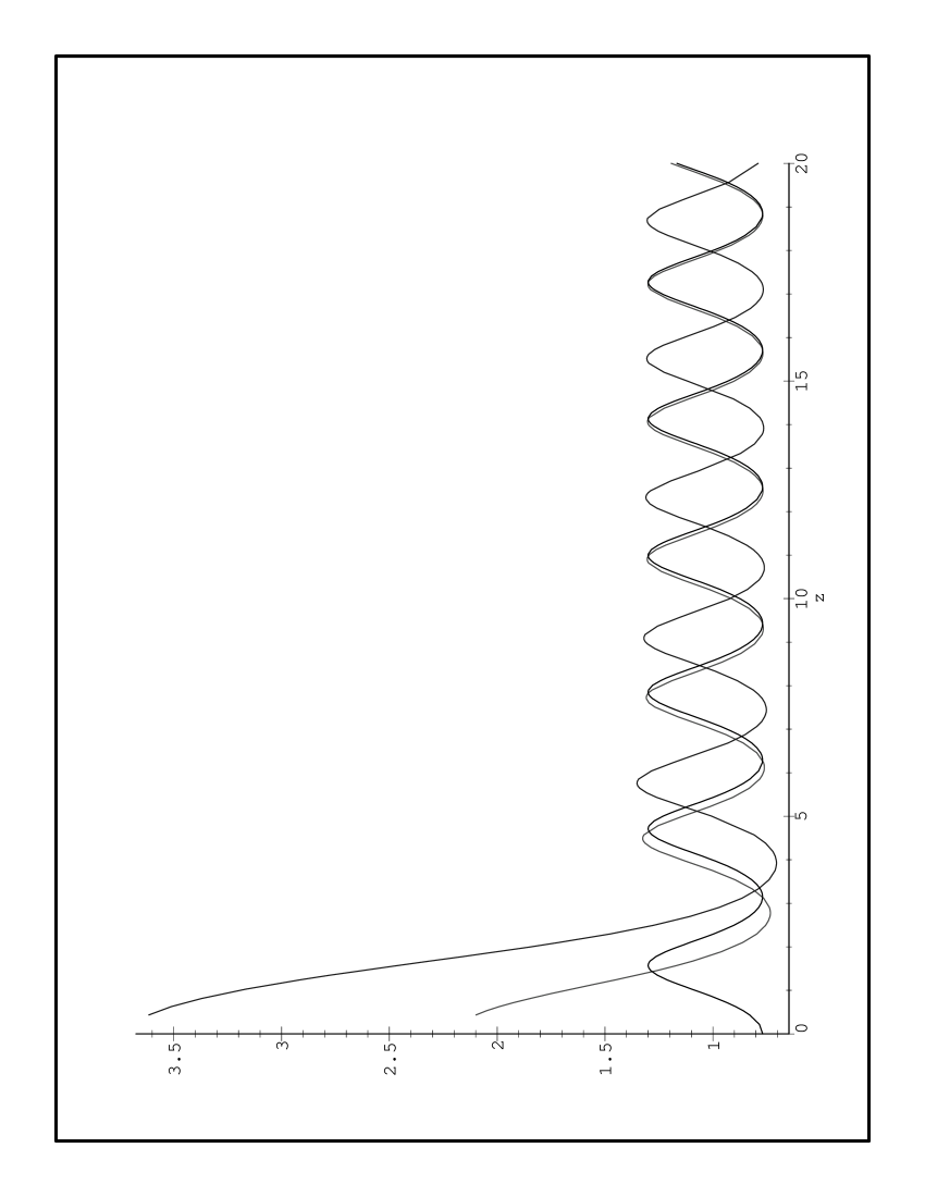
FIG. 1.: Plot of $|A_{l}|^{2}$ for $\nu=3/2$ and $\nu=5/2$. (Here we define $z=\omega R/c$ and put $n_{gas}=1$, $n_{liquid}=1.3$.) The function rapidly stabilizes to the asymptotic behavior. The dotted curve shows the behaviour of the asymptotic form for $\nu=3/2$.

We shall use this approximation to replace the $A_{\nu}$ factor with its mean value for large arguments:

$$|A_{\nu}|^{2}\approx{1\over 2\pi}\int_{0}^{2\pi}dz{2n_{gas}\,n_{liquid}\over n_{gas}^{2}+n_{liquid}^{2}+(n_{liquid}^{2}-n_{gas}^{2})\cos(z)}=1.$$ (83)

That this approximation is adequate may be checked a posteriori by seeing that the Bogolubov coefficients are not noticeably affected.

D The Pseudo-Wronskian

Use the simplified notation in which $x=n_{liquid}\,\omega_{out}R/c$, $y=n_{gas}\,\omega_{in}R/c$. In these dimensionless quantities, after including the approximation equation (83), and making explicit the dependence on $R$ and $c$, equation (46) takes the form:

$$\left|\beta(x,y)\right|^{2}=\frac{R^{2}}{c^{2}}\frac{(n_{liquid}^{2}-n_{gas}^{2})^{2}}{n_{liquid}^{2}\,n_{gas}^{2}}\left(\frac{y^{2}}{n_{gas}\,x+n_{liquid}\,y}\right)^{2}F(x,y).$$ (84)

Here $F(x,y)$ is shorthand for the function

$$F(x,y)=\sum_{l=1}^{\infty}(2l+1){\left|\begin{array}[]{rr}J_{\nu}(x)&J_{\nu}(y)\\ x\;J^{\prime}_{\nu}(x)&y\;J^{\prime}_{\nu}(y)\end{array}\right|^{2}\over(x^{2}-y^{2})^{2}},$$ (85)

where in this equation the primes now signify derivatives with respect to the full arguments ($x$ or $y$).

In order to proceed in our analysis we need now to perform the summation over angular momentum. Although the infinite sum is analytically intractable, there are two reasonable arguments (one physical and one mathematical) both leading to the conclusion that suitable truncations of this sum will be enough for our purposes.

The first argument is a physical one and it is based on the maximum amount of angular momentum that an outgoing photon may have. Basically, if one supposes the photons to be produced inside or at most on the surface of the bubble, the upper limit for the angular momentum will be the product of the bubble radius times the maximal “out” momentum. Then one gets:

$$l_{max}(K)={R(\hbar K)\over\hbar}=RK.$$ (86)

For sonoluminescence $K$ is of order $2\pi/(200{\rm nm})$. Deciding the appropriate value of $R$ is more tricky. Since the sonoluminescence flash occurs at or near the moment of minimum radius one might wish to use $R_{min}\approx 500{\rm nm}$ in which case $l_{max}(K)\approx 15$. Certainly for this choice of $R$ keeping the first ten or so terms will be sufficient. More conservatively, one might wish to choose $R$ to be of order $R_{ambient}\approx 4.5\mu m$ in which case $l_{max}(K)\approx 135$. Keeping this number of terms in the series is already very unwieldy. Finally, in Schwinger’s original version of the model it is the change in Casimir energy during the collapse all the way from maximum radius that is relevant, so perhaps one should use $R_{max}\approx 45\mu m$. In this case $l_{max}(K)\approx 1350$, and explicit summation of the series is prohibitively difficult. To handle these problems we develop a semi-analytic approximation to the sum which is sufficient for making numerical estimates of the spectrum.

This argument can be bolstered by considering the large order expansion ($\nu\rightarrow\infty$ at fixed $x$) of the Bessel functions. In this limit one gets [27]:

$$J_{\nu}(x)\sim{\frac{1}{\sqrt{2\pi\nu}}}\left(\frac{ex}{2\nu}\right)^{\nu}$$ (87)

This can be used to obtain the asymptotic form of the pseudo-Wronskian appearing in equation (85).

$$\tilde{W}_{\nu}(x,y) \equiv \left|\begin{array}[]{rr}J_{\nu}(x)&J_{\nu}(y)\\ x\;J^{\prime}_{\nu}(x)&y\;J^{\prime}_{\nu}(y)\end{array}\right|$$ (90)

$$= -\left|\begin{array}[]{rr}J_{\nu}(x)&J_{\nu}(y)\\ x\;J_{\nu+1}(x)&y\;J_{\nu+1}(y)\end{array}\right|$$ (93)

$$\sim \frac{(x^{2}-y^{2})}{2\pi(\nu)^{1/2}(\nu+1)^{3/2}}\left(\frac{xy}{\nu(\nu+1)}\right)^{\nu}\left(\frac{e}{2}\right)^{2\nu+1}.$$ (94)

where we have used the standard recursion relation for the Bessel functions $J^{\prime}_{\nu}(z)=\nu J_{\nu}(z)-zJ_{\nu+1}(z)$. This indicates that the sum over $\nu$ is convergent: the terms for which $(xy/\nu^{2})\leq 1$ are suppressed. Since, depending on one’s views as to the appropriate value of $R$, $x$ and $y$ are at most of order $15$, $135$, or $1350$ we deduce that the maximal contribution to the sum comes from a limited number of terms.

Analytically, it is easy to see that the function $F(x,y)$ is finite along the diagonal and goes smoothly to zero for $x,y\rightarrow 0$. To proceed to an actual computation of the predicted spectrum we need to develop an semi-analytic approximate form for this function by considering separately the behaviour along the diagonal $x-y=0$ and in the transversal direction $x+y={\rm constant}$.

E Working along the diagonal

To study in more detail the behaviour of such a function in this zone one can perform a Taylor expansion of $F(x,y)$ around $x=y$.

$$\lim_{x\rightarrow y}\frac{\tilde{W}_{\nu}(x,y)}{(x-y)} \equiv \lim_{x\rightarrow y}\frac{\left|\begin{array}[]{rr}J_{\nu}(x)&J_{\nu}(y)\\ x\;J^{\prime}_{\nu}(x)&y\;J^{\prime}_{\nu}(y)\end{array}\right|}{(x-y)}$$ (97)

$$= \lim_{x\rightarrow y}\frac{\left|\begin{array}[]{ll}J_{\nu}(x)&\hphantom{x\;}J_{\nu}(x)+(x-y)J^{\prime}_{\nu}(x)\\ x\;J^{\prime}_{\nu}(x)&x\;J^{\prime}_{\nu}(x)+(x-y)[J^{\prime}_{\nu}(x)+x\;J^{\prime\prime}_{\nu}(x)]\end{array}\right|}{(x-y)}$$ (100)

$$= \left|\begin{array}[]{rl}J_{\nu}(x)&J^{\prime}_{\nu}(x)\\ x\;J^{\prime}_{\nu}(x)&J^{\prime}_{\nu}(x)+x\;J^{\prime\prime}_{\nu}(x)\end{array}\right|$$ (103)

$$= J_{\nu}(x)[J^{\prime}_{\nu}(x)+x\;J^{\prime\prime}_{\nu}(x)]-x\;{J^{\prime}_{\nu}(x)}^{2}.$$ (104)

The derivatives can be eliminated by using the well known recursion relations.

$$\lim_{x\rightarrow y}\frac{\tilde{W}_{\nu}(x,y)}{(x-y)} = J_{\nu}(x)\left[\frac{(\nu^{2}-x^{2})}{x}\right]-x\;\left[\frac{\nu}{x}J_{\nu}(x)-J_{\nu+1}(x)\right]^{2}$$ (105)

$$= 2\nu J_{\nu}(x)J_{\nu+1}(x)-x\;\left[J_{\nu}^{2}(x)+J_{\nu+1}^{2}(x)\right].$$ (106)

For sake of simplicity we shall use an equivalent form of equation (106) where lower order Bessel function appear

$$\lim_{x\rightarrow y}\frac{\tilde{W}_{\nu}(x,y)}{(x-y)}=2\nu J_{\nu}(x)J_{\nu-1}(x)-x\;\left[J_{\nu}^{2}(x)+J_{\nu-1}^{2}(x)\right].$$ (107)

This result shows that, as expected, each term of $F(x,x)$ is finite along the diagonal and equal to zero at $x=y=0$. Moreover

$$D(x)\equiv F(x,x)=\sum_{l=1}^{\infty}(2l+1){\left\{(2l+1)J_{l+1/2}(x)J_{l-1/2}(x)-x\;\left[J_{l+1/2}^{2}(x)+J_{l-1/2}^{2}(x)\right]\right\}^{2}\over 4x^{2}}.$$ (108)

This sum can easily be checked to be convergent for fixed $x$. [Use equation (87).] With a little more work it can be shown that

$\displaystyle\lim_{x\to\infty}D(x)={1\over 2\pi^{2}}.$

The truncated function obtained after summation over the first few terms (say the first ten or so terms) is a long and messy combination of trigonometric functions that can however be easily plotted and approximated in the range of interest. Due to numerical artifacts, the function is not controllable near the origin, fortunately we have analytic information in that region — the function is very near to zero in the range $(0,1)$ for both “out” and “in” frequencies, and can be approximated by zero without any undue influence on the numerical results. A semi-analytical study led us to the approximate form of $D(x)$

$$D(x)\approx\Theta(x-1)\;\frac{1}{2\pi^{2}}\frac{2(x-1)^{2}}{3+2(x-1)^{2}}.$$ (109)

A confrontation between the two curves in the range of interest is given in the figure below.

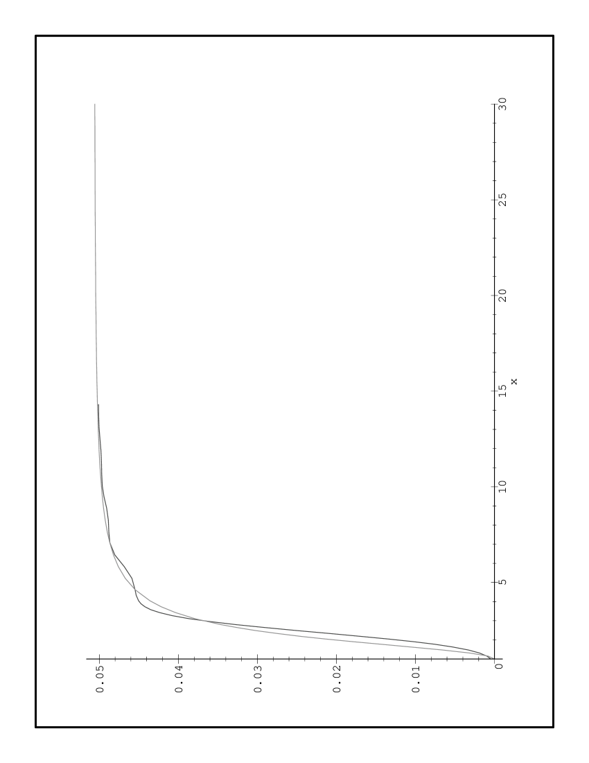
FIG. 2.: Plot of the exact $D(x)$ against its approximated form in the range $1<x<30$

F The factorization approximation

To numerically perform the integrals needed to do obtain the spectrum it is useful to note the approximate factorization property

$$F(x,y)\approx F\left({x+y\over 2},{x+y\over 2}\right)\;G\left(\frac{x-y}{2}\right).$$ (110)

That is: to a good approximation $F(x,y)$ is given by its value along the nearest part of the diagonal, multiplied by a universal function of the distance away from the diagonal. A little experimental curve fitting is actually enough to show that to a good approximation

$$F(x,y)\approx D\left({x+y\over 2}\right)\;{\sin^{2}(\pi[x-y]/4)\over(\pi[x-y]/4)^{2}}.$$ (111)

From the plot we show below it is easy to check that the function $F(x,y)$ is quite well fitted by our approximation. We feel important to stress that this is approximation is based on numerical experimentation, and is not an analytically-driven approximation. (In the infinite volume case we know that $F(x,y)\to(constant)\times\delta(x-y)$, cf. equation (64). The effect of finite volume is effectively to “smear out” the delta function. The combination $\sin^{2}(x)/(\pi x^{2})$ is one of the standard approximations to the delta function.) Our approximation is quite good everywhere except for values of $x$ and $y$ near the origin (less than 1) where the contribution of the function to the integral is very small.

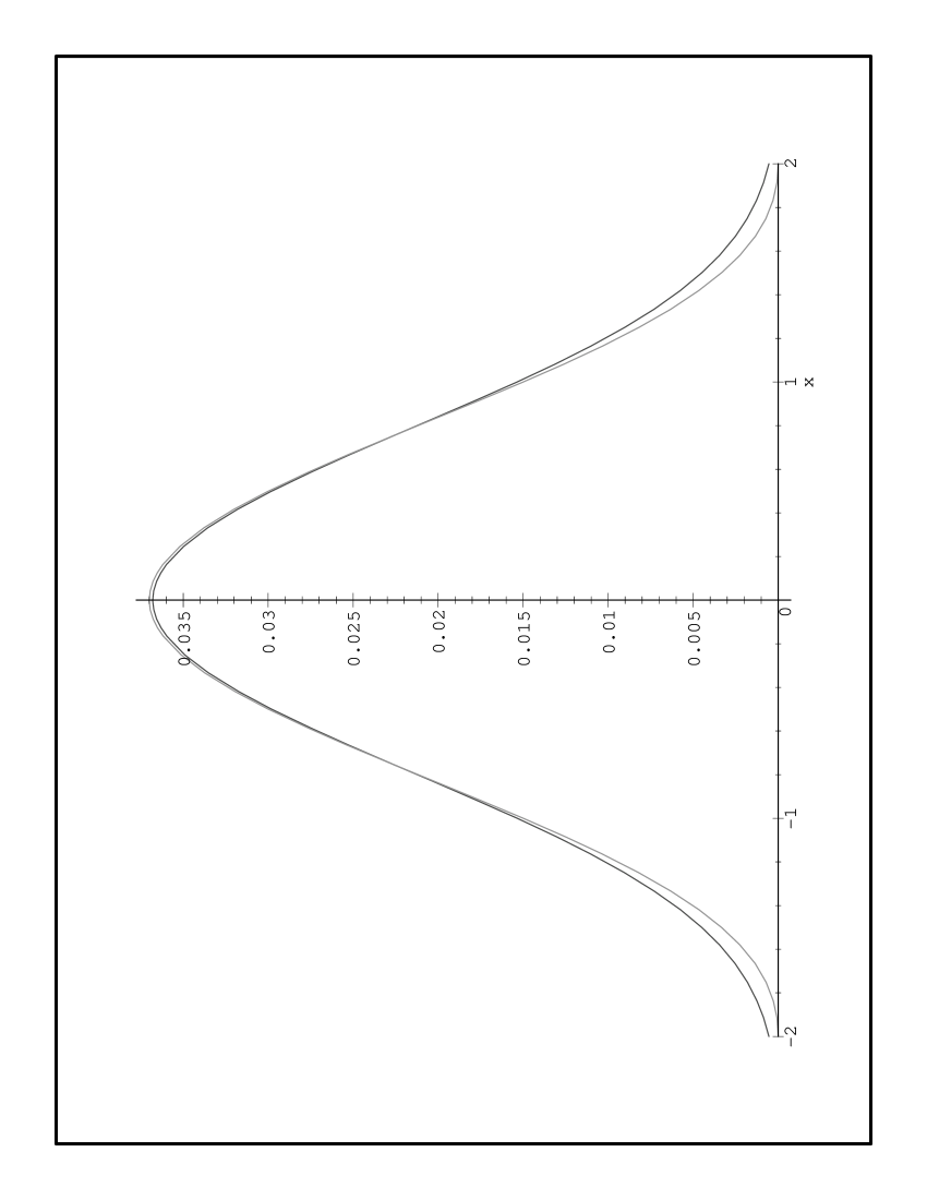
FIG. 3.: Transverse fit: An orthogonal slice of $F(x,y)$ intersecting the diagonal at $(x,y)=(3,3)$. Here $F(3+z,3-z)$ is plotted in comparison with $[\sin^{2}(\pi z/2)]/(\pi z/2)^{2}$.

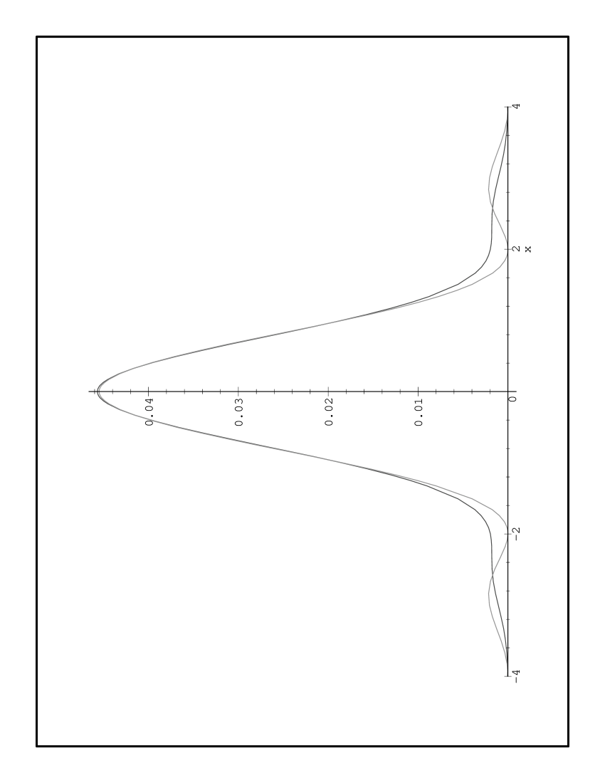
FIG. 4.: Transverse fit: An orthogonal slice of $F(x,y)$ intersecting the diagonal at $(x,y)=(5,5)$. Here $F(5+z,5-z)$ is plotted in comparison with $[\sin^{2}(\pi z/2)]/(\pi z/2)^{2}$.

FIG. 5.: Transverse fit: An orthogonal slice of $F(x,y)$ intersecting the diagonal at $(x,y)=(10,10)$. Here $F(10+z,10-z)$ is plotted in comparison with $[\sin^{2}(\pi z/2)]/(\pi z/2)^{2}$.

G The spectrum: numerical evaluation

We have now transformed the function $F(x,y)$ into an easy to handle product of two functions

$$F(x,y)\approx\Theta(x+y-2)\;\frac{1}{2\pi^{2}}\;\frac{(x+y-2)^{2}}{6+(x+y-2)^{2}}\;{\sin^{2}(\pi[x-y]/4)\over(\pi[x-y]/4)^{2}}.$$ (112)

We exhibit tridimensional graphs for both the exact (apart from the approximation of truncating the sum at a finite $l$) and approximate forms of the function $F(x,y)$. We have chosen the case of $R=0.5\mu{\rm m}$ (corresponding to $y_{max}=2.5$ as previously explained).

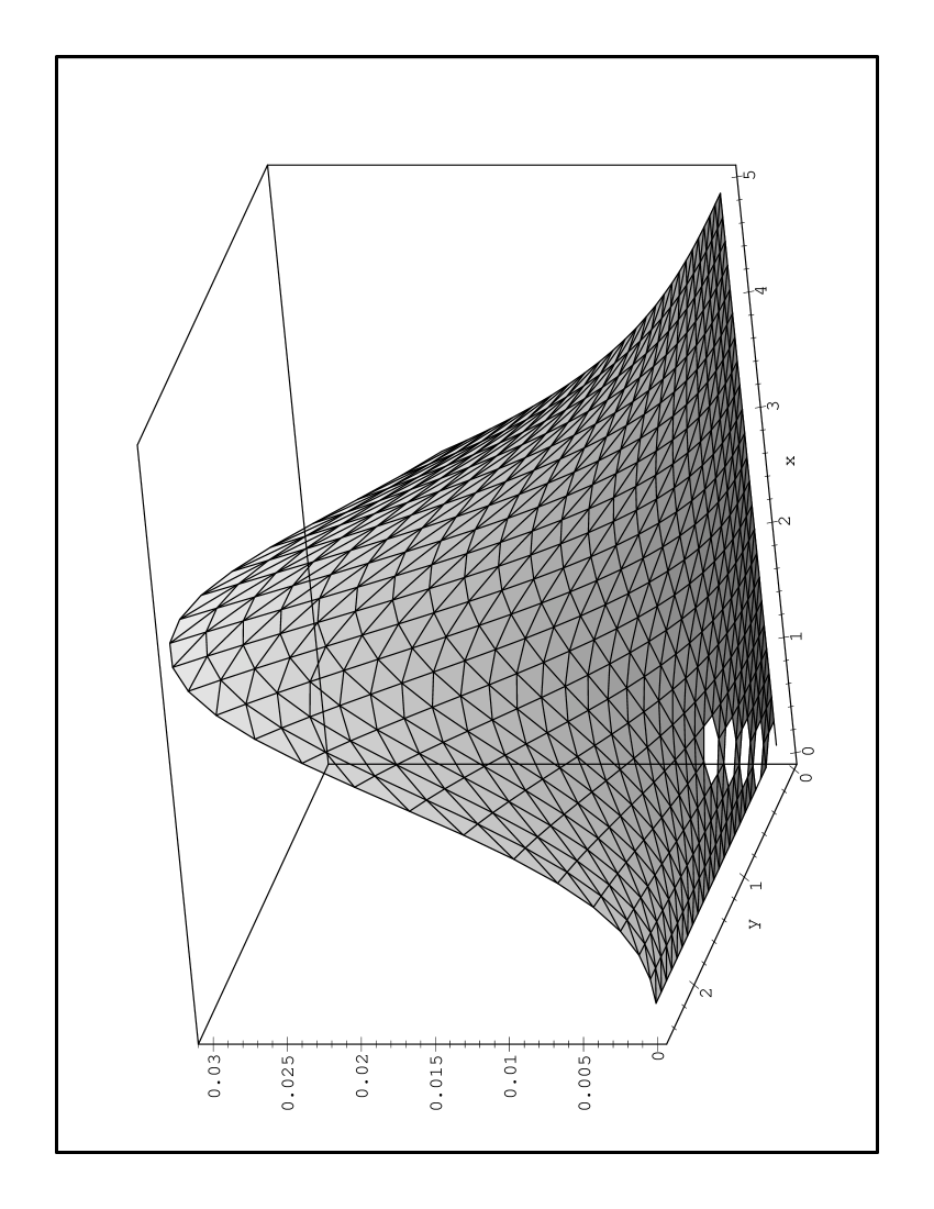
FIG. 6.: Plot of the exact $F(x,y)$ in the range $0<x<5$, $0<y<2.5$

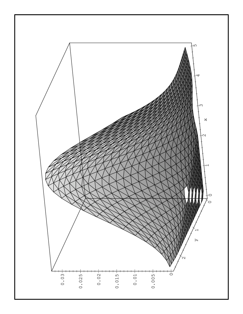
FIG. 7.: Plot of the approximated $F(x,y)$ in the range $0<x<5$, $0<y<2.5$

A numerical study of the error due to the replacement of $F(x,y)$ with its approximated form equation (112), leads to an upper limit of $20\%$ error in the total energy emitted.

The dimensionless spectrum, based on equations (46) and (84), is

$${dN\over dx}=\frac{(n_{liquid}^{2}-n_{gas}^{2})^{2}}{n_{liquid}^{3}\,n_{gas}^{3}}\int_{0}^{RK}\left(\frac{y^{2}}{n_{gas}\,x+n_{liquid}\,y}\right)^{2}D\left({x+y\over 2}\right){\sin^{2}(\pi[x-y]/4)\over(\pi[x-y]/4)^{2}}dy.$$ (113)

As a consistency check, the infinite volume limit is equivalent to making the formal replacements

$${\sin^{2}(\pi[x-y]/4)\over(\pi[x-y]/4)^{2}}\to 4\delta(x-y),$$ (114)

and

$$D\left({x+y\over 2}\right)\to{1\over 2\pi^{2}}.$$ (115)

Doing so, equation (113) reduces to equation (68) up to an overall factor [$4/\pi$] of order one. The correct dependence on refractive index and correct power-law behaviour for the spectrum are recovered, and the overall order one factor is merely a reflection of the crudity of the cutoff in angular momentum used in deriving (68).

With this consistency check out of the way, it is now possible to perform the integral with respect to $y$ to estimate the spectrum for finite volume. For definiteness we set $n_{liquid}=1.3$ and $n_{gas}=1.0$, put $K=2\pi/(200nm)$, and pick $R=0.5\mu{\rm m}$ (corresponding to $y_{max}=15$). We integrate from $y=0$ to $y=15$ and plot the resulting spectrum from $x=0$ to $x=18$.

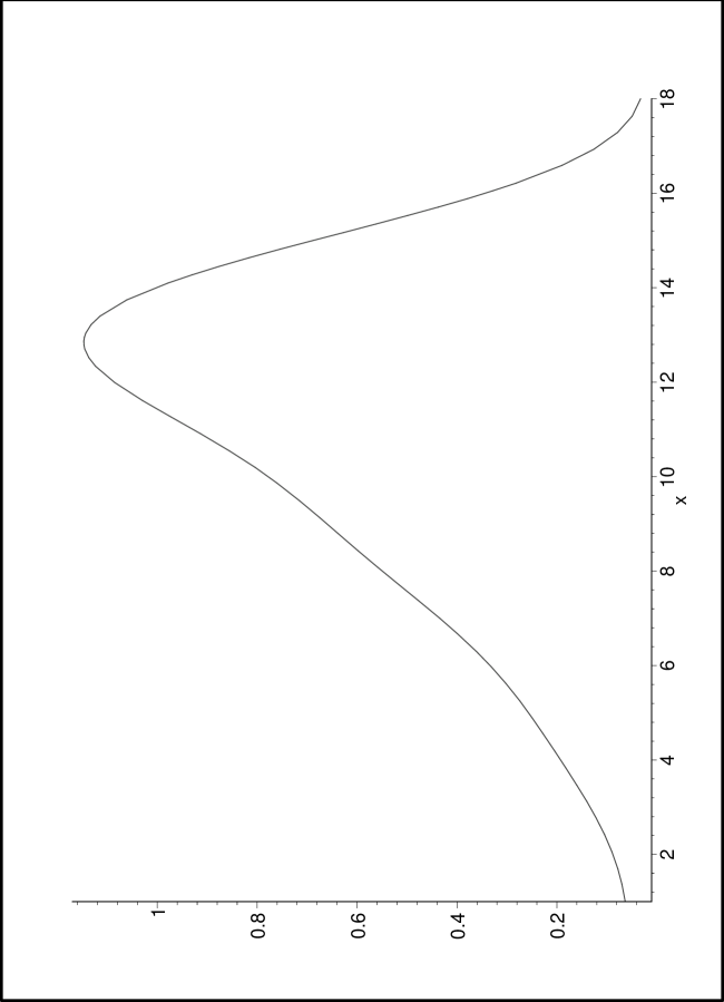
FIG. 8.: Spectrum obtained by the approximated Bogolubov coefficient for $R=0.5\mu{\rm m}$ corresponding to $y_{max}=15$. We integrate from $y=0$ to $y=15$ and plot the resulting spectrum from $x=0$ to $x=18$.

One can also ask what sort of result one would get if instead we pick a much larger value of $R$, say $R=5\mu m$, corresponding to the bubble at equilibrium radius. In this case the approach towards the Schwinger (infinite volume result) result is much closer. We now have $y_{max}=135$. We integrate from $y=0$ to $y=135$ and plot the resulting spectrum from $x=0$ to $x=140$. For comparison we plot it together with equation (68) which is Schwinger’s naive model (the re-scaled infinite volume limit).

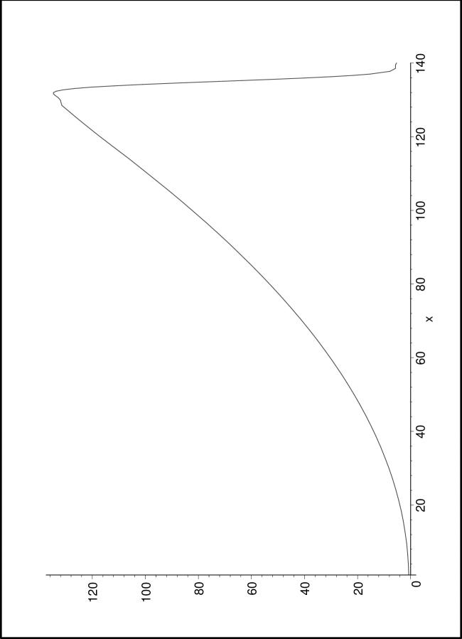
FIG. 9.: Spectrum obtained by the approximated Bogolubov coefficient for $R=5\mu{\rm m}$ corresponding to $y_{max}=135$. We integrate from $y=0$ to $y=135$ and plot the resulting spectrum from $x=0$ to $x=140$.

The case corresponding to the bubble at maximum radius, $R=50\mu m$, requires a range of integration too large for standard numerical plotting. In any case the graph will only be a replica of the previous one on a larger scale.

III Discussion

The lessons we have learned from this test calculation are:

—(1) The model proves (in an indirect way) that the Casimir energy produced via the bubble collapse includes (in the large $R$ limit) a term proportional to the volume (actually to the volume over which the refractive index changes). In the case of a truly dynamical model one expects that the energy of the photons so created will be provided by other sources of energy (e.g., the sound wave), nevertheless the presence of a volume contribution appears unavoidable.

—(2) The present model is still unable to fully fit other experimental features of sonoluminescence. For example it provides maximal photon release at maximum expansion. Barber et al. [12] point out that in Schwinger’s original model the main production of photons may be expected when the the rate of change of the volume is maximum, which is experimentally found to occur near the maximum radius. In contrast the emission of light in sonoluminescence is experimentally found to occur near the point of minimum radius, where the rate of change of area is maximum. All else being equal, this would seem to indicate a surface dependence and might be interpreted as a true weakness of the dynamical Casimir explanation of sonoluminescence.

In fact we have shown elsewhere [13, 14, 15, 16] that the situation is considerably more complex than might naively be thought. It is important to stress that what Schwinger proposed was clearly only a first estimate of the vacuum energy, which was in principle viable as the basis for a model, and not a fully dynamical model. Schwinger was fully aware of this in his papers.

A fully dynamical calculation is required in order to deal with these issues, and the experimental data give remarkable suggestions about the plausible directions for theoretical developments within the framework of the dynamic Casimir effect. In particular, one of the key features of photon production by a space-dependent and time-dependent refractive index is that for a change occurring on a timescale $\tau$, the amount of photon production is exponentially suppressed by an amount $\exp(-\omega\tau)$. In [14] we have provided a specific model that exhibits this behaviour, and argued that the result is in fact generic. The importance for sonoluminescence is that the experimental spectrum is not  exponentially suppressed at least out to the far ultraviolet. Therefore any mechanism of Casimir-induced photon production based on an adiabatic approximation is destined to failure: Since the exponential suppression is not visible out to $\omega\approx 10^{15}\;\hbox{Hz}$, it follows that if  sonoluminescence is to be attributed to photon production from a time-dependent dielectric bubble (i.e., the dynamical Casimir effect), then the timescale for change in the refractive index must be of order of a femtosecond. Thus any Casimir–based model has to take into account that it is no longer the collapse from $R_{\mathrm{m}ax}$ to $R_{\mathrm{m}in}$ that is important. One has to divorce the change in refractive index from direct coupling to the bubble wall motion, and instead ask for a rapid change in the refractive index of the entrained gases as they are compressed down to their van der Waals hard core [14, 15]. We stress that this conclusion, though it moves away from the original Schwinger proposal, is still firmly within the realm of the dynamic Casimir effect approach to sonoluminescence. The fact is that the present work shows clearly that a viable Casimir “route” to sonoluminescence cannot avoid a “fierce marriage” between QFT and features related to condensed matter physics.

IV Conclusions

The present calculation unambiguously verifies that a sudden change in radius of a dielectric bubble causes a change in the Casimir energy that is, as predicted by Schwinger [8, 20, 21, 22], converted into real photons with a phase space spectrum. As far as sonoluminescence is concerned, we have also explained why such a change must be sudden in order to fit the experimental data. This leads us to propose a somewhat different model of sonoluminescence based on the dynamical Casimir effect, a model focussed on the actual dynamics of the refractive index (as a function of space and time), and not just of the bubble boundary. (In Schwinger’s original approach the refractive index changes only due to motion of the bubble wall.) In summary, provided the sudden approximation is valid, changes in the refractive index will lead to efficient conversion of zero point fluctuations into real photons. Trying to fit the details of the observed spectrum in sonoluminescence then becomes an issue of building a robust model of the refractive index of both the ambient water and the entrained gases as functions of frequency, density, and composition. Only after this prerequisite is satisfied will we be in a position to develop a more complex dynamical model endowed with adequate predictive power.

In light of these observations we think that one can also derive a general conclusion about the long standing debate on the actual value of the static Casimir energy and its relevance to sonoluminescence: Sonoluminescence is not directly related to the static Casimir effect. The static Casimir energy is at best capable of giving a crude estimate for the energy budget in sonoluminescence.

REFERENCES

- [1] E-mail: liberati@sissa.it
- [2] E-mail: visser@kiwi.wustl.edu
- [3] E-mail: belgiorno@mi.infn.it
- [4] E-mail: sciama@sissa.it
- [5] J. Schwinger, Proc. Nat. Acad. Sci. 89, 4091–4093 (1992).
- [6] J. Schwinger, Proc. Nat. Acad. Sci. 89, 11118–11120 (1992).
- [7] J. Schwinger, Proc. Nat. Acad. Sci. 90, 958–959 (1993).
- [8] J. Schwinger, Proc. Nat. Acad. Sci. 90, 2105–2106 (1993).
- [9] J. Schwinger, Proc. Nat. Acad. Sci. 90, 4505–4507 (1993).
- [10] J. Schwinger, Proc. Nat. Acad. Sci. 90, 7285–7287 (1993).
- [11] J. Schwinger, Proc. Nat. Acad. Sci. 91, 6473–6475 (1994).
- [12] B.P. Barber, R.A. Hiller, R. Löfstedt, S.J. Putterman Phys. Rep. 281, 65-143 (1997).
- [13] S. Liberati, M. Visser, F. Belgiorno, and D.W. Sciama, Sonoluminescence: Bogolubov coefficients for the QED vacuum of a collapsing bubble, quant-ph/9805023, to appear in Physical Review Letters.
- [14] S. Liberati, M. Visser, F. Belgiorno, and D.W. Sciama, Sonoluminescence as a QED vacuum effect. I: Physical Scenario, quant-ph/9904013.
- [15] S. Liberati, M. Visser, F. Belgiorno, and D.W. Sciama, Sonoluminescence as a QED vacuum effect. II: Finite Volume Effects, quant-ph/9905034.
- [16] F. Belgiorno, S. Liberati, M. Visser, and D.W. Sciama, Sonoluminescence: Two-photon correlations as a test for thermality, quant-ph/9904018.
- [17] C. Eberlein, Sonoluminescence as quantum vacuum radiation, Phys. Rev. Lett. 76, 3842 (1996). quant-ph 9506023
- [18] C. Eberlein, Theory of quantum radiation observed as sonoluminescence, Phys. Rev. A 53, 2772 (1996). quant-ph 9506024
- [19] C. Eberlein, Sonoluminescence as quantum vacuum radiation (reply to comment), Phys. Rev. Lett. 78, 2269 (1997). quant-ph/9610034
- [20] C. E. Carlson, C. Molina–París, J. Pérez–Mercader, and M. Visser, Phys. Lett. B 395, 76-82 (1997). hep-th/9609195
- [21] C. E. Carlson, C. Molina–París, J. Pérez–Mercader, and M. Visser, Phys. Rev. D56, 1262 (1997). hep-th/9702007.
- [22] C. Molina–París and M. Visser, Phys. Rev. D56, 6629 (1997). hep-th/9707073.
- [23] K. Milton, Casimir energy for a spherical cavity in a dielectric: toward a model for Sonoluminescence?, in Quantum field theory under the influence of external conditions, edited by M. Bordag, (Tuebner Verlagsgesellschaft, Stuttgart, 1996), pages 13–23. See also hep-th/9510091.
- [24] K. Milton and J. Ng, Casimir energy for a spherical cavity in a dielectric: Applications to Sonoluminescence, hep-th/9607186.
- [25] K. Milton and J. Ng, Observability of the bulk Casimir effect: Can the dynamical Casimir effect be relevant to Sonoluminescence ?, hep-th/9707122.
- [26] H. Bateman, Higher Transcendental Functions, Vol II, (McGraw-Hill, New York, 1953).
- [27] A. Jeffrey, Handbook of Mathematical Formulas and Integrals, page 219, (Academic Press, San Diego, 1995).