Recoil and momentum diffusion of an atom close to a vacuum-dielectric interface

Abstract

We derive the quantum-mechanical master equation (generalized optical Bloch equation) for an atom in the vicinity of a flat dielectric surface. This equation gives access to the semiclassical radiation pressure force and the atomic momentum diffusion tensor, that are expressed in terms of the vacuum field correlation function (electromagnetic field susceptibility). It is demonstrated that the atomic center-of-mass motion provides a nonlocal probe of the electromagnetic vacuum fluctuations. We show in particular that in a circularly polarized evanescent wave, the radiation pressure force experienced by the atoms is not colinear with the evanescent wave’s propagation vector. In a linearly polarized evanescent wave, the recoil per fluorescence cycle leads to a net magnetization for a $J_{g}=1/2$ ground state atom.

submitted to European Physical Journal D

PACS numbers: 32.80.P – radiation pressure, 03.75.Be – atom optics, 42.50.V – mechanical effects of light on atoms

I Introduction

When an atom is absorbing or emitting light, its center-of-mass is subject to photon recoil. This phenomenon, already pointed out by Einstein in the early years of the century [1], is the core ingredient of the atomic motion manipulation techniques that have attracted much attention during the last 20 years [2, 3, 4, 5]. Quite paradoxically, however, this basic ingredient embodies its own limit, as it also provides crucial limiting factors to the performances of these techniques. For example, the minimum attainable temperatures in laser cooling are generally limited by the random fluctuations in the momenta exchanged between photons and atoms, that give rise to atomic momentum diffusion [1, 2, 3, 4]; also in the most promising field of atom optics [6], spontaneous emission represents a lethal threat to the coherence of the de Broglie waves because the atomic wave vector acquires an indeterminacy due to the random photon recoil [7].

In this paper, we study the recoil effects due to spontaneous emission in the vicinity of a vacuum–dielectric interface for an atom being reflected from an evanescent wave. This atom-optical device is one of the most studied realizations of a coherent mirror for atomic de Broglie waves [8, 9, 10, 11, 12]. Being based upon the interaction between an atom and an evanescent laser wave propagating along the surface of a dielectric prism, it already allowed for detailed experimental investigations of fluorescence rates [13, 14], single optical pumping cycles [15, 16] and ground-state energy shifts [17] at distances of order $\lambdabar=c/\omega_{A}$ from the interface ($\omega_{A}$ is the atomic transition frequency). Spontaneous emission in the evanescent wave is also used in reflection cooling techniques [15, 16, 18] that have been proposed for radiative atom traps in the vicinity of surfaces [19, 20, 21, 22, 23, 24, 25]. From these experiments it has become apparent that a proper description of the fluorescence rates and the energy levels has to take into account the distortion of the electromagnetic field due to the presence of the dielectric. A precise theory of the atom–light interaction in the evanescent wave mirror hence touches upon the field of cavity QED [26] and might even provide a model system for one of this field’s paradigms: that the radiative properties of an atom are determined by the local properties of the electromagnetic field at the atom’s position. In fact, as far as the ‘internal’ atomic dynamics (spontaneous emission rates and frequency shifts) is concerned, this problem has already been studied intensively, starting from the work of Drexhage [27] and Chance et al. [28] and covering a variety of geometries and materials (dielectric or metallic) [29, 30, 31, 32, 33, 34, 35, 36, 37, 38, 39, 40]. In a recent paper, Courtois et al. [41] calculated the cavity QED modifications to the optical Bloch equations that govern the relaxation processes of a multilevel atom close to the vacuum–dielectric interface. This study showed that the relaxation due to spontaneous emission is determined by the radiative damping rates of classical dipoles located near the interface. The paper was limited, however, to atoms at rest: only the internal dynamics was treated, whereas the ‘external dynamics’ (recoil of the atomic center-of-mass) had still to be included. The present paper intends to fill this gap: we derive the so-called generalized optical Bloch equations that describe both internal and external dynamics of an atom in the vicinity of the vacuum–dielectric interface. We actually start from a more general perspective and determine, for a generic cavity geometry, the master equation for the atomic density matrix, including the center-of-mass degrees of freedom. The modifications of the electromagnetic vacuum field appear in this equation through the field correlation function, taken at two spatially separated positions. It hence turns out that the atomic external degrees of freedom constitute a nonlocal probe of the spatial correlations of the electromagnetic cavity field. We then follow the general procedure outlined by Dalibard and Cohen-Tannoudji [5] and use the Wigner representation to express the spatial dependence of the atomic density matrix in terms of a phase-space quasi-distribution. In the semiclassical limit, the atomic Wigner function evolves according to a Fokker–Planck equation where appear the radiation pressure force and the momentum diffusion, and these quantities involve spatial derivatives of the field correlation function. In free space, this is simply a reformulation of the random momentum exchanges between the atom, the laser field, and the vacuum field [42]. In a cavity-type geometry, on the other hand, photons do not rapidly escape to infinity, and the spatial structure of the field modes becomes important for the atomic recoil.

We illustrate the capabilities of the Bloch–Fokker–Planck equation derived in this paper by focusing on spontaneous emission in the evanescent wave mirror. In particular, some unusual properties of the radiation pressure force above the dielectric interface are displayed. As a first example, we show that it differs from the naive estimate based upon the phase gradient of the evanescent driving field and the spontaneous emission rate. More explicitly, if the evanescent wave is circularly polarized, the radiation pressure force points into a different direction than the (real part of the) evanescent field’s wave vector. This is due to the fact that the vacuum–dielectric interface partially reflects the electromagnetic field and hence modifies the spatial structure of the vacuum fluctuations. From the viewpoint of radiation reaction, the correction to the radiation pressure corresponds to the force exerted by the atom’s dipole field that is backreflected from the interface. As a second example, we study the optical pumping of a $J_{g}=1/2$ atom in the vicinity of the dielectric. The reduced symmetry of the electromagnetic vacuum field implies that the average recoil per optical pumping cycle differs between the two Zeeman sublevels, even in a linearly polarized evanescent field. As a consequence, an initially unpolarized atomic ensemble splits into two spin components with different average momentum after a pumping cycle. For some velocity classes the sublevel populations then have become imbalanced, and the atomic ensemble shows what may be called a ‘recoil-induced magnetization’.

The theory outlined in this paper thus improves previous ‘heuristic’ approaches to atomic recoil in evanescent waves [13, 43, 44], that assume the atomic fluorescence to be distributed according to the free-space dipole radiation pattern. Our results are also relevant for radiative atom traps in the vicinity of material surfaces [19, 20, 21, 22, 23, 24, 25], where momentum diffusion due to spontaneous emission may be one of the limiting factors for the temperature. While current atomic mirror experiments are typically limited to the transient regime, such traps would allow to study the radiation pressure force in evanescent waves in the long-time limit (steady state). From a more general perspective, the framework presented here may also be used to predict the center-of-mass motion of cold atoms in a high-finesse optical cavity with its electromagnetic field modes being confined both in real and frequency space. It is an interesting result for the domain of cavity QED that the external motion of atoms in a cavity provides a nonlocal probe of the cavity field correlation function, in opposition to internal radiative properties that are determined by the field correlations at the same point. The examples we develop demonstrate that this direction of cavity QED may be investigated with current experiments.

The paper is organized as follows: in Sec. II, we present the generalized optical Bloch equations including a nontrivial correlation function for the electromagnetic vacuum field. We focus on atoms driven by a monochromatic field in the low-saturation, large-detuning limit. Eliminating adiabatically the excited state, the Bloch equations reduce to the optical pumping equation involving only the ground state density matrix. Passing to the Wigner representation, these equations take the form of a Fokker–Planck equation in the semiclassical limit. We display general expressions for the radiation pressure force and the momentum diffusion tensor that apply to any Zeeman degeneracy. The conditions of validity for our approach are summarized. In Sec. III, the example of the evanescent wave mirror allows us to illustrate the general theory. We discuss the reduced symmetry of the electromagnetic field correlations in the vacuum above a flat dielectric surface and recover, in the absence of recoil, the well-known fluorescence rates for this geometry. Specializing to a scalar ground state, i.e., a $J_{g}=0\rightarrow J_{e}=1$ atom, we study the influence of the evanescent wave’s polarization on the radiation pressure force and the momentum diffusion tensor. We then consider a $J_{g}=1/2$ ground state atom and examine optical pumping in the evanescent wave. The appendixes contain several technical results that are used in the text.

II Generalized optical Bloch equations

The internal and external dynamics of an atom interacting with a laser field are conveniently characterized by a master equation for its density matrix (generalized optical Bloch equation ‘G.O.B.E.’). This section is devoted to the derivation of such an equation in the particular case of a multilevel atom located close to the interface between vacuum and a dielectric medium.

A General

To begin, we identify the general features of the G.O.B.E. at an interface. In free space, the master equation describing the interaction of a single multilevel atom with a monochromatic laser field is well-known [45, 46]. Basically, its derivation proceeds in two steps. In the first step, one considers the evolution equation for the total density matrix of the system constituted by the atom and the electromagnetic field. In the framework of nonrelativistic quantum electrodynamics and in the electric dipole approximation, this equation relies upon the atom-field Hamiltonian

$$H=H_{0}+H_{R}+V_{AL}+V_{AR}$$ (1)

The first term on the right-hand side of Eq.(1) is the atomic Hamiltonian accounting for the internal energy energy of the bare atom and for its kinetic energy:

$$H_{0}=\frac{{\bf P}^{2}}{2M}+\frac{\hbar\omega_{0}}{2}(P_{e}-P_{g})$$ (2)

where ${\bf P}$ is the atomic momentum operator, $M$ is the atomic mass, and $P_{g}$ and $P_{e}$ are the projection operators on the ground and excited states, respectively; the second term is the free Hamiltonian of the Coulomb-gauge quantized electromagnetic field; $V_{AL}$ is the time-dependent, purely atomic Hamiltonian

$$V_{AL}=-{\bf D}.{\cal\vec{E}}_{L}\left({\bf R},t\right)$$ (3)

that describes the interaction of the atomic dipole ${\bf D}$ with the laser field assumed to be in a coherent state and therefore described by a classical function ${\cal\vec{E}}_{L}\left({\bf r},t\right)$; and the last term,

$$V_{AR}=-{\bf D}.{\bf E}({\bf R})$$ (4)

represents the coupling between the atom and the reservoir associated with the vacuum quantum field ${\bf E(R})$. We note that in Eq.(1), both fields ${\cal\vec{E}}_{L}\left({\bf R},t\right)$ and ${\bf E(R})$ are evaluated at the location of the atom (${\bf R}$: atomic center-of-mass position operator). In the second step, the master equation for the atomic density matrix $\rho$ is obtained by applying second order perturbation theory to the atom-reservoir interaction, and by tracing away the degrees of freedom associated with the reservoir. This yields a dynamical evolution equation where the influence of the reservoir is manifest through two contributions. The first, associated with an effective Hamiltonian, describes the energy shifts undergone by the atomic levels as a result of their coupling to the vacuum field (Lamb-shifts). These shifts are traditionally assimilated in the definition of $H_{0}$, yielding the actual atomic Hamiltonian $H_{A,\infty}$. The second contribution, $\dot{\rho}_{relax,\infty}$, represents the dissipation of the atomic system due to its coupling with the reservoir (spontaneous emission). Finally, the free-space time evolution of the atomic density matrix takes the form

$$\dot{\rho}={\cal L}_{\infty}\,\rho$$ (5)

$${\cal L}_{\infty}\,\rho=\frac{1}{i\hbar}\left[H_{A,\infty}+V_{AL},\rho\right]+\dot{\rho}_{relax,\infty}$$ (6)

where we have introduced the free-space Liouville operator ${\cal L}_{\infty}$ .

We now consider an atom located in the vicinity of a vacuum-dielectric interface. What are the modifications of the master equation (5) induced by the lower-lying dielectric medium? First, because of the new boundary conditions, the modes of ${\cal\vec{E}}_{L}\left({\bf r},t\right)$ and of the quantized electromagnetic vacuum field are altered and may become evanescent. It is clear that this does not affect the operators $H_{0}$, $H_{R}$, and $V_{AL}$ which keep the same form as in the free-space case. In contrast, the structure of the reservoir becomes modified. The contributions of $V_{AR}$ to the atom dynamics (energy level shifts and spontaneous emission rates) are therefore expected to be different from the free-space situation. Moreover, as a result of the instantaneous Coulomb interaction between the atomic and dielectric charges, one expects a supplementary electrostatic contribution $H_{es}$ to the energy level shifts. $H_{es}$ corresponds to the London-Van der Waals interaction of the instantaneous atomic dipole with its image in the dielectric medium (higher multipoles can be neglected provided the atomic radius is much less than the distance between the atom and the dielectric surface). Finally, denoting by $\Delta H_{A}$ and $\dot{\rho}_{relax,int}$ the modifications of the Hamiltonian and dissipative parts of the atomic density matrix evolution due to the interface, one obtains the general form of the G.O.B.E. in the presence of the dielectric medium

$$\dot{\rho}={\cal L}_{\infty}\,\rho+{\cal L}_{int}\,\rho$$ (7)

where

$${\cal L}_{int}\,\rho=\frac{1}{i\hbar}\left[\Delta H_{A},\rho\right]+\dot{\rho}_{relax,int}$$ (8)

entirely describes the influence of the interface on the atomic dynamics. In particular, ${\cal L}_{int}\,\rho$ tends toward zero when the atom is far from the dielectric surface. The expression of the atomic level shifts close to a vacuum-dielectric interface have been presented in Ref. [41] and will not be discussed any further. We will therefore only focus on the dissipative contribution to Eq.(8).

B Master equation treatment of spontaneous emission

We consider the relaxation processes undergone by the atom as a result of its coupling with the vacuum quantum field. As is well-known, these processes are conveniently described by a master equation for the atomic density matrix. In this section, we derive such an equation taking into account the presence of the lower-lying dielectric medium.

1 Atom-quantum field coupling

As stated above, the coupling between the atom and the quantized electromagnetic field (which is responsible for spontaneous emission) is described by the Hamiltonian $V_{AR}=-{\bf D.E(R})$. The atomic dipole operator ${\bf D}$ changes sign under parity, and therefore has only zero matrix elements inside the Zeeman degeneracy subspaces of both the ground and excited states. Furthermore, because $\left|g\right\rangle$ and $\left|e\right\rangle$ have well-defined angular momenta, it is possible following the Wigner-Eckart theorem to write ${\bf D}$ in terms of a dimensionless, reduced dipole operator ${\bf d}$

$${\bf D}={\cal D\,}{\bf d}$$ (9)

whose matrix elements contain the Clebsch-Gordan coefficients associated with the addition of the angular momenta $1+J_{g}\rightarrow J_{e}$. In Eq.(9), ${\cal D}$ is a real number characterizing the electric dipole moment amplitude of the atomic transition. We further decompose the reduced dipole operator as

$${\bf d=}P_{e}\,{\bf d\,}P_{g}+P_{g}\,{\bf d\,}P_{e}={\bf d}^{+}+{\bf d}^{-}$$ (10)

and expand ${\bf d}^{+}$ and ${\bf d}^{-}=\left({\bf d}^{+}\right)^{\dagger}$ onto the standard basis $\{{\bf u}_{\pm 1}=\mp\left({\bf e}_{x}\pm\,i{\bf e}_{y}\right)/\sqrt{2},{\bf u}_{0}={\bf e}_{z}\}$ (where ${\bf e}_{x,y,z}$ are the unitary vectors associated with the cartesian coordinate system)

$$d_{q}^{+}={\bf d}^{+}.{\bf u}_{q}=\left(d_{q}^{-}\right)^{\dagger}$$ (11)

The matrix elements of $d_{q}^{+}$ are then given by the simple expression

$$\left\langle J_{e}\,M_{e}\right|d_{q}^{+}\left|J_{g}\,M_{g}\right\rangle=\left\langle J_{g}\,1\,M_{g}\,q\right|J_{e}\,M_{e}\rangle$$ (12)

where $\left\langle J_{g}\,1\,M_{g}\,q\right|J_{e}\,M_{e}\rangle$ is the Clebsch-Gordan coefficient connecting the Zeeman sublevels $\left|J_{g}\,M_{g}\right\rangle$ and $\left|J_{e}\,M_{e}=M_{g}+q\right\rangle$. Finally, using the rotating-wave approximation, the interaction Hamiltonian $V_{AR}$ takes the more explicit form

$$V_{AR}=-{\cal D}\sum\limits_{q=-1}^{1}\left(d_{q}^{+}{\,}E_{q}^{+}+d_{q}^{-}\,E_{q}^{-}\right)$$ (13)

where

$${\bf E}^{+}=\sum\limits_{q=-1}^{1}E_{q}^{+}\,{\bf u}_{q}=\left({\bf E}^{-}\right)^{\dagger}$$ (14)

is the positive-frequency component of the electric field operator.

2 Relaxation equation for the atomic density matrix

The total contribution $\dot{\rho}_{relax}=\dot{\rho}_{relax,\infty}+\dot{\rho}_{relax,int}$ of spontaneous emission to the time evolution of the atomic density matrix can be readily derived from the standard procedure [29, 45, 46, 47] outlined in Appendix A, where it is shown that in spite of the quantization of the center-of-mass motion, $\dot{\rho}_{relax}$ is of the familiar form, being a sum of two terms

$$\left\langle{\bf r}_{1}\right|\dot{\rho}_{relax}\left|{\bf r}_{2}\right\rangle = -\frac{\Gamma_{\infty}}{2}\left\langle{\bf r}_{1}\right|\left\{C^{i,j}({\bf R},{\bf R})\,d_{i}^{+}\,d_{j}^{-}\,,\rho\right\}\left|{\bf r}_{2}\right\rangle$$ (16)

$$+\Gamma_{\infty}\,C^{i,j}({\bf r}_{2},{\bf r}_{1})\,\,d_{j}^{-}\,\left\langle{\bf r}_{1}\right|\rho\left|{\bf r}_{2}\right\rangle\,d_{i}^{+}$$

where $\left\{A,B\right\}=AB+BA$ denotes the anti-commutator between operators $A$ and $B$,

$$\Gamma_{\infty}=\frac{{\cal D}^{2}\omega_{0}^{3}}{3\pi\varepsilon_{0}\,\hbar\,c^{3}}$$ (17)

is the natural linewidth of the excited state in free space, and where a sum is to be taken over the $i,j=x,y,z$ indices. The first line of Eq.(16) describes the relaxation of the populations and Zeeman coherences of the excited state and of the optical coherences due to spontaneous emission. It involves the dimensionless tensor $C^{i,j}({\bf r}_{1},{\bf r}_{2})$, proportional to the Fourier transform of the electromagnetic vacuum field correlation function at the atomic transition frequency $\omega_{0}$

$$\Gamma_{\infty}C^{i,j}({\bf r}_{1},{\bf r}_{2})=\frac{{\cal D}^{2}}{\hbar^{2}}\int\limits_{-\infty}^{\infty}\!d\tau\,e^{i\omega_{0}\tau}\langle 0|E_{i}^{+}({\bf r}_{1},\tau)E_{j}^{-}({\bf r}_{2},0)|0\rangle$$ (18)

where $\left|0\right\rangle$ denotes the vacuum state of the field. The second line in Eq.(16) describes the feeding of the ground-state Zeeman sublevels by spontaneous emission, yielding the expected population conservation relation $\mathop{\rm Tr}\,\left(\dot{\rho}_{relax}\right)=0$.

It is clearly apparent in Eq.(16) that the effect of the dielectric medium on the atomic relaxation is entirely described by the correlation tensor $C^{i,j}({\bf r}_{1},{\bf r}_{2})$ previously derived by Carnaglia and Mandel [48] (a useful representation of $C^{i,j}({\bf r}_{1},{\bf r}_{2})$ is given in Appendix C). Finally, we note that in the case where the atom is infinitely far from the vacuum-dielectric interface, the correlation tensor $C^{i,j}({\bf r}_{1},{\bf r}_{2})$ reduces to its free-space value [49], and Eq.(16) transforms into its well-known expression:

$$\left\langle{\bf r}_{1}\right|\dot{\rho}_{relax,\infty}\left|{\bf r}_{2}\right\rangle$$ (19)

$$=-\frac{\Gamma_{\infty}}{2}\left\langle{\bf r}_{1}\right|\left\{P_{e}\,,\rho\right\}\left|{\bf r}_{2}\right\rangle+\Gamma_{\infty}\,\int\frac{d^{2}{\bf n}}{8\pi/3}\,\sum_{\mathchoice{{\hbox{\boldmath$\displaystyle\varepsilon$}}}{{\hbox{\boldmath$\textstyle\varepsilon$}}}{{\hbox{\boldmath$\scriptstyle\varepsilon$}}}{{\hbox{\boldmath$\scriptscriptstyle\varepsilon$}}}\bot{\bf n}}$$ (20)

$$\quad\left({\bf d}^{-}.\mathchoice{{\hbox{\boldmath$\displaystyle\varepsilon$}}}{{\hbox{\boldmath$\textstyle\varepsilon$}}}{{\hbox{\boldmath$\scriptstyle\varepsilon$}}}{{\hbox{\boldmath$\scriptscriptstyle\varepsilon$}}}^{*}\right)\,e^{-i{\bf k.r}_{1}}\,\left\langle{\bf r}_{1}\right|\rho\left|{\bf r}_{2}\right\rangle e^{i{\bf k.r}_{2}}\,\left({\bf d}^{+}.\mathchoice{{\hbox{\boldmath$\displaystyle\varepsilon$}}}{{\hbox{\boldmath$\textstyle\varepsilon$}}}{{\hbox{\boldmath$\scriptstyle\varepsilon$}}}{{\hbox{\boldmath$\scriptscriptstyle\varepsilon$}}}\right)$$ (21)

where ${\bf n}$ is a unit vector and ${\bf k}$ is defined by ${\bf k=(}\omega_{0}{\bf/}c{\bf)n}$.

C Evolution of the ground state density matrix in the Wigner representation

In this section, the G.O.B.E. (7) is transformed into a Fokker–Planck-type equation for the phase-space distribution function of the atomic ground state. First, we eliminate adiabatically the optical coherences $\rho_{eg}=P_{e}\,\rho\,P_{g}$, $\rho_{ge}=P_{g}\,\rho\,P_{e}$ and the excited state density matrix $\rho_{ee}=P_{e}\,\rho\,P_{e}$ by expressing them in terms of the ground-state density matrix $\rho_{gg}=P_{g}\,\rho\,P_{g}\equiv\sigma$. This approximation, which holds in the limit of large laser frequency detunings from resonance and low saturation of the atomic transition, presents the advantage of reducing the atomic dynamics to a single Zeeman manifold (optical pumping equation). In a second step, we Wigner-transform the ground-state density operator $\sigma$. In the new representation, $\sigma$ is represented by a $(2J_{g}+1)\times(2J_{g}+1)$ matrix $W({\bf r,p},t)$, particularly well suited to the investigation of the semiclassical limit of the atomic motion [3, 5].

1 Adiabatic elimination of the excited state

In laser cooling or atom optics experiments, it is customary to operate in conditions of large laser frequency detuning from resonance and low saturation of the atomic transition. These conditions allow one to perform the adiabatic elimination of both the optical coherences $\rho_{eg}$, $\rho_{ge}$ and the excited state density matrix $\rho_{ee}$. As shown in Appendix B, this elimination amounts to the following substitutions. First, the dipole operators ${\bf d}^{\pm}$ are replaced by

$${\bf d}^{-}\mapsto{\bf b}^{-}({\bf R})={\bf d}^{-}\left[{\bf d}^{+}\cdot\mathchoice{{\hbox{\boldmath$\displaystyle\xi$}}}{{\hbox{\boldmath$\textstyle\xi$}}}{{\hbox{\boldmath$\scriptstyle\xi$}}}{{\hbox{\boldmath$\scriptscriptstyle\xi$}}}({\bf R})\right]$$ (22)

$${\cal\vec{E}}_{L}({\bf r})={\cal E}_{0}\,\mathchoice{{\hbox{\boldmath$\displaystyle\xi$}}}{{\hbox{\boldmath$\textstyle\xi$}}}{{\hbox{\boldmath$\scriptstyle\xi$}}}{{\hbox{\boldmath$\scriptscriptstyle\xi$}}}({\bf r})$$ (23)

with ${\bf b}^{\pm}({\bf R})$ being hermitian conjugates. The non-normalized, dimensionless vector $\mathchoice{{\hbox{\boldmath$\displaystyle\xi$}}}{{\hbox{\boldmath$\textstyle\xi$}}}{{\hbox{\boldmath$\scriptstyle\xi$}}}{{\hbox{\boldmath$\scriptscriptstyle\xi$}}}({\bf r})$ specifies the laser spatial profile and polarization, while ${\cal E}_{0}$ gives the order of magnitude of the electric field amplitude.

The second replacement involves the caracteristic timescale of the ground-state density matrix elements: the spontaneous emission rate $\Gamma_{\infty}$ is replaced by the typical photon scattering rate $\Gamma_{\infty}^{\prime}$

$$\Gamma_{\infty}\mapsto\Gamma_{\infty}^{\prime}=\Gamma_{\infty}\frac{s_{0}}{2}$$ (24)

where

$$s_{0}=2\left(\frac{{\cal DE}_{0}}{\hbar\Delta}\right)^{2}\ll 1$$ (25)

is the saturation parameter in the large detuning limit $\left|\Delta=\omega_{L}-\omega_{0}\right|\gg\Gamma_{\infty}$.

Finally, using the usual rotating-wave approximation for $V_{AL}$ and by neglecting the influence of the atomic velocity on laser frequency detuning (Doppler effect), the G.O.B.E. (7) yields the optical pumping equation (see Appendix B):

$$\langle{\bf r}_{1}|\dot{\sigma}|{\bf r}_{2}\rangle = \frac{1}{i\hbar}\langle{\bf r}_{1}|\left[\frac{{\bf P}^{2}}{2M}+H_{eff}({\bf R}),\,\sigma\right]|{\bf r}_{2}\rangle$$ (28)

$$-\frac{\Gamma_{\infty}^{\prime}}{2}\langle{\bf r}_{1}|\left\{{\cal G}({\bf R}),\sigma\right\}|{\bf r}_{2}\rangle$$

$$+\,\Gamma_{\infty}^{\prime}\,C^{i,j}({\bf r}_{2},{\bf r}_{1})b_{j}^{-}({\bf r}_{1})\langle{\bf r}_{1}|\sigma|{\bf r}_{2}\rangle b_{i}^{+}({\bf r}_{2})$$

where

$$H_{eff}({\bf R}) = P_{g}\,\Delta H_{A}({\bf R})\,P_{g}$$ (30)

$$+\hbar\Delta^{\prime}\,\left({\bf d}^{-}\cdot\mathchoice{{\hbox{\boldmath$\displaystyle\xi$}}}{{\hbox{\boldmath$\textstyle\xi$}}}{{\hbox{\boldmath$\scriptstyle\xi$}}}{{\hbox{\boldmath$\scriptscriptstyle\xi$}}}^{*}({\bf R})\right)\left({\bf d}^{+}\cdot\mathchoice{{\hbox{\boldmath$\displaystyle\xi$}}}{{\hbox{\boldmath$\textstyle\xi$}}}{{\hbox{\boldmath$\scriptstyle\xi$}}}{{\hbox{\boldmath$\scriptscriptstyle\xi$}}}({\bf R})\right)$$

is the effective Hamiltonian accounting for the dielectric-induced energy level shifts of the ground state (first term on the right-hand side) and the ground-state light shifts (last term), the order of magnitude of which is

$$\hbar\Delta^{\prime}=\hbar\Delta\,\frac{s_{0}}{2}$$ (31)

We also introduced in (28) the ground-state operator

$${\cal G}({\bf r})=C^{i,j}({\bf r},{\bf r})b_{i}^{+}({\bf r})b_{j}^{-}({\bf r})$$ (32)

Besides, to first order in $\Gamma_{\infty}/\Delta$, the connection between $\sigma$ and the optical coherences and excited-state parts of the density matrix can be readily expressed in the following form (see Appendix B):

$$\langle{\bf r}_{1}|\rho_{eg}|{\bf r}_{2}\rangle=\langle{\bf r}_{2}|\rho_{ge}|{\bf r}_{1}\rangle^{\dagger}=$$ (33)

$$\quad=-\frac{{\cal DE}_{0}}{\hbar\Delta}\left(\delta^{i,j}-i\frac{\Gamma_{\infty}}{2\Delta}C^{i,j}({\bf r}_{1},{\bf r}_{1})\,\right)\times$$ (34)

$$\quad\quad\times d_{i}^{+}b_{j}^{-}({\bf r}_{1})\,\langle{\bf r}_{1}|\sigma|{\bf r}_{2}\rangle\,e^{-i\omega_{L}t}$$ (35)

$$\langle{\bf r}_{1}|\rho_{ee}|{\bf r}_{2}\rangle=\frac{s_{0}}{2}\,\left({\bf d}^{+}\cdot\mathchoice{{\hbox{\boldmath$\displaystyle\xi$}}}{{\hbox{\boldmath$\textstyle\xi$}}}{{\hbox{\boldmath$\scriptstyle\xi$}}}{{\hbox{\boldmath$\scriptscriptstyle\xi$}}}({\bf r}_{1})\right)\langle{\bf r}_{1}|\sigma|{\bf r}_{2}\rangle\left({\bf d}^{-}\cdot\mathchoice{{\hbox{\boldmath$\displaystyle\xi$}}}{{\hbox{\boldmath$\textstyle\xi$}}}{{\hbox{\boldmath$\scriptstyle\xi$}}}{{\hbox{\boldmath$\scriptscriptstyle\xi$}}}^{*}({\bf r}_{2})\right)$$ (36)

where $\delta^{i,j}$ is the Kronecker symbol. The validity conditions of the expressions given in this section are detailed in section II C 3.

2 Wigner representation of the ground state density matrix

a General.

The Wigner representation of the density matrix provides a particularly convenient framework for the intuitive understanding of atomic motion in laser light. This is because beside its intrinsic quasi-probability distribution character, which often enables to map classical pictures onto phenomena of quantum nature such as the atomic recoil induced by absorption or emission of photons, the Wigner representation is the best suited for taking advantage of the general characteristics of laser-cooled atomic samples to exhibit momentum widths $\Delta p$ significantly larger than the photon momentum $\hbar k$, that characterizes the elementary step of the momentum random walk experienced by the atom as a result from its momentum exchanges with the laser field.

More quantitatively, the time evolution of the Wigner representation $W({\bf r},{\bf p},t)$ of the ground state atomic density matrix

$$W({\bf r},{\bf p},t)=\frac{1}{(2\pi\hbar)^{3}}\int\!d^{3}s\,\sigma({\bf r};{\bf s})\exp{(-}i{\bf p}.{{\bf s}/\hbar)}$$ (37)

$$\sigma({\bf r};{\bf s})\equiv\left\langle{\bf r}+{\textstyle\frac{1}{2}}{\bf s}|\sigma|{\bf r}-{\textstyle\frac{1}{2}}{\bf s}\right\rangle$$ (38)

can be deduced from the optical pumping equation (28). One thus finds after a straightforward calculation:

$$\frac{\partial W}{\partial t}({\bf r},{\bf p},t)=-\frac{{\bf p}}{M}\cdot\nabla_{{\bf r}}W({\bf r},{\bf p},t)+$$ (39)

$$+\int\!\frac{d^{3}{\bf s}}{(2\pi\hbar)^{3}}e^{-i{\bf p}.{\bf s}/\hbar}\times$$ (40)

$$\times\bigg{(}\frac{1}{i\hbar}\left[H_{eff}({\bf r}+{\textstyle\frac{1}{2}}{\bf s})\sigma({\bf r};{\bf s})-\sigma({\bf r};{\bf s})H_{eff}({\bf r}-{\textstyle\frac{1}{2}}{\bf s})\right]$$ (41)

$$-\frac{\Gamma_{\infty}^{\prime}}{2}\left\{{\cal G}({\bf r}+{\textstyle\frac{1}{2}}{\bf s})\sigma({\bf r};{\bf s})+\sigma({\bf r};{\bf s}){\cal G}({\bf r}-{\textstyle\frac{1}{2}}{\bf s})\right\}$$ (42)

$$+\Gamma_{\infty}^{\prime}C^{i,j}({\bf r};{\bf s})b_{j}^{-}({\bf r}+{\textstyle\frac{1}{2}}{\bf s})\sigma({\bf r};{\bf s})b_{i}^{+}({\bf r}-{\textstyle\frac{1}{2}}{\bf s})\bigg{)}$$ (43)

where

$$C^{i,j}({\bf r};{\bf s})\equiv C^{i,j}\left({\bf r}-{\textstyle\frac{1}{2}}{\bf s},{\bf r}+{\textstyle\frac{1}{2}}{\bf s}\right)$$ (44)

Because the different quantities inside the integral exhibit an ${\bf s}$ dependence, Eq.(43) clearly connects $\partial_{t}W({\bf r},{\bf p},t)$ to some others $W({\bf r},{\bf p}+\delta{\bf p},t)$, which is reminiscent from the recoil of the atom during photon absorption or emission processes, hence $\left|\delta{\bf p}\right|\approx\hbar k$. Because $\hbar k/\Delta p\ll 1$, Eq.(43) can be accurately evaluated by expanding $W({\bf r},{\bf p}+\delta{\bf p},t)$ up to second order in $\delta{\bf p}$ [5]. A more direct way of implementing this procedure is to note that $\hbar k/\Delta p\ll 1$ implies that the coherence length of the atomic ensemble, $\hbar/\Delta p$, is small compared to the optical wavelength $\lambda=2\pi/k$. This implies that the width in ${\bf s}$ of the external coherence function $\sigma({\bf r};{\bf s})$ is small compared to the scale of variation of the quantities $C^{i,j}({\bf r}-\frac{1}{2}{\bf s},{\bf r}+\frac{1}{2}{\bf s})$ and ${\bf b}^{\pm}({\bf r}\pm\frac{1}{2}{\bf s})$, which is of the order of $\lambda$. It is therefore possible to expand directly the integral kernel of Eq.(43) up to second order in $k{\bf s}$ before evaluating the integral. We now discuss more quantitatively this procedure in order to identify the influence of the vacuum-dielectric interface on the atomic dynamics.

b Zeroth order: internal atomic dynamics.

The lowest (zeroth) order in the expansion of the different quantities in the integration kernel of Eq.(43) amounts to considering the atoms as point-like particles, i.e., to treating the atomic translational degrees of freedom classically. It is therefore not surprising to end with the previously-established optical pumping equation [41] for a point atom having a constant velocity ${\bf p}/M$ which yields, after adiabatic elimination of the excited state and optical coherences:

$${\cal O}[(k{\bf s})^{0}]:\quad\left.\frac{\partial W}{\partial t}\right|_{0} = -\frac{{\bf p}}{M}\cdot\nabla_{{\bf r}}W+$$ (46)

$$+\frac{1}{i\hbar}\left[H_{eff}({\bf r}),\,W\right]+\left.\dot{W}_{relax}\right|_{0}$$

where the effective Hamiltonian $H_{eff}$ only impacts on the evolution of the ground state Zeeman coherences (the space dependence of $H_{eff}$ has no effect on the atomic motion to zeroth order in $k{\bf s\,}$) and where

$$\left.\dot{W}_{relax}\right|_{0} = -\frac{\Gamma_{\infty}^{\prime}\,}{2}C^{i,j}({\bf r};{\bf 0})\{b_{i}^{+}({\bf r})\,b_{j}^{-}({\bf r}),\,W\}+$$ (48)

$$+\Gamma_{\infty}^{\prime}\,C^{i,j}({\bf r};{\bf 0})\,b_{j}^{-}({\bf r})\,W\,b_{i}^{+}({\bf r})$$

accounts for departure from the ground-state through laser absorption (first term on the right-hand side) and for feeding of the ground-state by spontaneous emission (second term), the combined action of which yields optical pumping. Eq.(48) shows that the optical pumping or fluorescence rates are determined by the one-point correlation tensor $C^{i,j}({\bf r};{\bf 0})=C^{i,j}({\bf r},{\bf r})$. In free space, one has $C^{i,j}({\bf r};{\bf 0})=\delta^{i,j}$ so the position dependence of the fluorescence and optical pumping rates only arises from the driving field profile $\mathchoice{{\hbox{\boldmath$\displaystyle\xi$}}}{{\hbox{\boldmath$\textstyle\xi$}}}{{\hbox{\boldmath$\scriptstyle\xi$}}}{{\hbox{\boldmath$\scriptscriptstyle\xi$}}}({\bf r})$ [cf. Eq.(22)]. On the other hand, close to a vacuum–dielectric interface, as will be shown below, one has $C^{i,j}({\bf r};{\bf 0})=\delta^{i,j}c^{i}(z)$, so an additional cause for a spatially varying optical pumping rates appears. As already pointed out in Ref. [41], this phenomenon is directly connected to the well-known space-dependence of the damping rates of classical oscillating dipoles close to a vacuum-dielectric interface.

c First order: radiative and level shift-induced forces.

To first order in $k{\bf s}$, where the effect of the atom-field coupling on the atomic motion enters into play, the ground-state G.O.B.E.’s expansion takes the form of a Liouville equation uncovering the force ${\bf F}({\bf r})$ acting on the atom

$${\cal O}[(k{\bf s})^{1}]:\quad\left.\frac{\partial W}{\partial t}\right|_{1}+{\bf F}({\bf r})\cdot\nabla_{{\bf p}}W=0$$ (49)

The force operator ${\bf F}({\bf r})$ is actually the sum of three terms:

$${\bf F}={\bf F}^{(shift)}+{\bf F}^{(dip)}+{\bf F}^{(sp)}$$ (50)

where

$$\Big{(}{\bf F}^{(shift)}+{\bf F}^{(dip)}\Big{)}\cdot\nabla_{{\bf p}}W=-{\textstyle\frac{1}{2}}\left\{\nabla_{{\bf r}}H_{eff}({\bf r}),\,\nabla_{{\bf p}}W\right\}$$ (51)

involves the sum of the force associated with the dielectric-induced energy level shifts (${\bf F}^{(shift)}$) and of the dipole force (${\bf F}^{(dip)}$) associated with the ground-state light-shifts (${\bf F}^{(shift)}$ and ${\bf F}^{(dip)}$ are associated with the first and second term of Eq.(30), respectively), and where

$${\bf F}^{(sp)}={\bf F}_{\text{depart}}^{(sp)}+{\bf F}_{\text{feed}}^{(sp)}$$ (52)

is the radiation pressure force, having two contributions arising from each term of the right-hand side of Eq.(48), respectively. One finds:

$${\bf F}_{\text{feed}}^{(sp)}({\bf r})\cdot\nabla_{{\bf p}}W=-i\hbar\Gamma_{\infty}^{\prime}\nabla_{{\bf s}}{\cal A}({\bf r};{\bf 0})\cdot\nabla_{{\bf p}}W$$ (53)

where ${\cal A}({\bf r};{\bf s})$ is an operator involving the field correlation function at two points separated by ${\bf s}$, defined as

$${\cal A}({\bf r};{\bf s})\,W\equiv C^{i,j}({\bf r};{\bf s})\,b_{j}^{-}({\bf r}+{\textstyle\frac{1}{2}}{\bf s})\,W\,b_{i}^{+}({\bf r}-{\textstyle\frac{1}{2}}{\bf s})$$ (54)

and

$${\bf F}_{\text{depart}}^{(sp)}({\bf r})\cdot\nabla_{{\bf p}}W=\frac{i}{4}\hbar\Gamma_{\infty}^{\prime}\left[\nabla_{{\bf r}}{\cal G}({\bf r}),\nabla_{{\bf p}}W\right]$$ (55)

In order to make the physical content of ${\bf F}_{\text{feed}}^{(sp)}$ more transparent, let us consider the simple situation where the driving laser field is a plane wave of wavevector ${\bf q}$, in which case the operators ${\bf b}^{\pm}$ take the simple form

$${\bf b}^{\pm}({\bf r})={\bf\beta}_{0}^{\pm}\,e^{\mp i{\bf q.r}}$$ (56)

where ${\bf\beta}_{0}^{\pm}$ are space-independent operators. A straightforward calculation then yields

$${\bf F}_{\text{feed}}^{(sp)}({\bf r}).\nabla_{{\bf p}}W = \hbar\Gamma_{\infty}^{\prime}\left({\bf q\,}C^{i,j}({\bf r};{\bf 0})\right.$$ (58)

$$\left.-i\nabla_{{\bf s}}C^{i,j}({\bf r};{\bf 0})\right)\beta_{0j}^{-}.\nabla_{{\bf p}}W\,\beta_{0i}^{+}$$

Eq.(58) shows that ${\bf F}_{\text{feed}}^{(sp)}$ results from two contributions, the physical significance of which can be deduced by referring to the well-known free space situation: the first term in parentheses describes the atomic recoil $\hbar{\bf q}$ due to the absorption of the driving plane wave photons, while the second is associated with the atomic recoil during spontaneous emission. One can thus consider that the presence of the dielectric medium affects the quantitative value of ${\bf F}_{\text{feed}}^{(sp)}$ through the modification of $C^{i,j}({\bf r};{\bf 0})$, but that it remains qualitatively analogous to the free space situation.

The situation is quite different for ${\bf F}_{\text{depart}}^{(sp)}$. Considering Eqs. (55) and (32), one can indeed note that whereas in free space, the contribution to ${\bf F}_{\text{depart}}^{(sp)}$ only arises from the space dependence of the laser field, a supplementary contribution shows up in the vicinity of a vacuum-dielectric interface due to the space-dependence of the one-point correlation tensor $C^{i,j}({\bf r},{\bf r})$. In the preceding case of a plane wave driving field, whereas ${\bf F}_{\text{depart}}^{(sp)}$ reduces zero in free space, one thus obtains a purely dielectric-induced contribution (cancelling in free space) of the form:

$${\bf F}_{{\rm depart}}^{(sp)}.\nabla_{{\bf p}}W=\frac{i}{4}\hbar\Gamma_{\infty}^{\prime}\nabla_{{\bf r}}C^{i,j}({\bf r};{\bf 0}).\left[\beta_{0i}^{+}\beta_{0j}^{-},\nabla_{{\bf p}}W\right]$$ (59)

d Second order: momentum diffusion tensor.

To second order in $k{\bf s}$, we find a Fokker–Planck equation for the Wigner matrix. Its diffusion term is given by

$\displaystyle{\cal O}[(k{\bf s})^{2}]:\quad\left.\frac{\partial W}{\partial t}\right|_{2}=D^{k,l}({\bf r})\frac{\partial^{2}W}{\partial p_{k}\partial p_{l}}$

The momentum diffusion tensor

$$D^{k,l}({\bf r})=D_{\text{depart}}^{k,l}+D_{\text{feed}}^{k,l}$$ (60)

again contains contributions from the departure and feeding terms on the right-hand side of Eq.(48), respectively:

$$D_{\text{depart}}^{k,l}\frac{\partial^{2}W}{\partial p_{k}\partial p_{l}}=\frac{\hbar^{2}\Gamma_{\infty}^{\prime}}{16}\left\{\frac{\partial^{2}{\cal G}}{\partial r_{k}\partial r_{l}},\frac{\partial^{2}W}{\partial p_{k}\partial p_{l}}\,\right\}$$ (61)

$$D_{\text{feed}}^{k,l}=-\,\frac{\hbar^{2}\Gamma_{\infty}^{\prime}}{2}\frac{\partial^{2}{\cal A}}{\partial s_{k}\partial s_{l}}({\bf r};{\bf 0})$$ (62)

As it is well-known [50], this tensor results from various phenomena: randomness of atomic recoil processes due to laser absorption and stimulated/spontaneous emission, spatial spreading or shrinking of the atomic wavepacket due to the space variation of the absorption or optical pumping rates. Because the dielectric medium affects both, absorption and spontaneous emission processes, one expects modifications of the atomic momentum diffusion in the vicinity of the vacuum-dielectric interface.

3 Validity conditions of the derivations

To conclude this section, we summarize the validity conditions for our approach. The mose stringent condition arises from our approximation that the excited state density matrix adiabatically follows the ground state density matrix. This means first that the atoms move little on the scale $\lambdabar$ during the lifetime $1/\Gamma_{\infty}$ of the excited state, or equivalently:

$$\Gamma_{\infty}\gg\frac{kp}{M},\,\frac{k\Delta p}{M}$$ (63)

Second, the force $F_{e}$ acting on the excited state must be sufficiently small that during the lifetime $1/\Gamma_{\infty}$, the shift of the atomic momentum is negligible compared to the width $\Delta p$ of the momentum distribution:

$$\Gamma_{\infty}\gg\frac{F_{e}}{\Delta p}$$ (64)

Under typical experimental conditions (distance $z\sim 1/k$), the force $F_{e}$ is at most of order [31] ${\cal D}^{2}/\varepsilon_{0}z^{4}\sim\hbar k\Gamma_{\infty}/(kz)^{4}\sim\hbar k\Gamma_{\infty}$. Condition (64) hence reduces to the semiclassical regime $\Delta p\gg\hbar k$ we shall suppose throughout this article [cf. condition (66) below].

The elimination of the optical coherences is governed by a different condition: the laser detuning $\Delta$ must be larger than any other frequency scale in the G.O.B.E. (cf. Appendix B)

$$|\Delta|\gg\Gamma_{\infty},\,\frac{{\cal DE}_{0}}{\hbar},\,\frac{kp}{M},\,\frac{|\Delta H_{A}|}{\hbar}$$ (65)

This condition implies a small saturation parameter (22) and amounts to neglecting the Doppler shift of the laser frequency. It also allows to discard the dielectric-induced shift of the atomic transition frequency compared to the free-space detuning (see Ref. [41] for more details).

Furthermore, since $\omega_{A}\gg|\Delta|$ (near-resonant excitation), the atomic dynamics is ‘frozen’ at the timescale of the vacuum field correlation time. This justifies the Markov approximation made in deriving the G.O.B.E. (16). We note that if the conditions (63, 65) are relaxed, one has to take into account both the ground- and the excited-state manifolds, with spontaneous emission inducing transitions between them. This picture is reminiscent of the dressed-state description [51] and has been used, e.g., in Refs.[13, 19].

As pointed out in Subsec. II C 2 above, the mechanical effects of spontaneous emission may be described simply in a semiclassical way if the atomic momentum distribution varies smoothly on the scale of the photon momentum

$$\Delta p\gg\hbar k$$ (66)

Combining with condition (63), our approach is limited to transitions with $\Gamma_{\infty}\gg\omega_{\text{recoil}}\equiv\hbar k^{2}/2M$. It therefore fails for light atoms like He or Li, e.g., while it applies for heavier atoms like Na, Ne^∗, Ar^∗, Rb, Cs …

III Atomic motion at an evanescent wave mirror

In this section, we illustrate the capabilities of the approach developed above by applying it to the motion of an atom in an evanescent wave mirror, in the vicinity of a vacuum–dielectric interface. We first examine the electromagnetic field correlation tensor in this geometry, with particular emphasis on its symmetry properties. We thus recover the well-known atomic damping rates above the dielectric interface. The radiation pressure force and the momentum diffusion tensor are then explicitly calculated for a $J_{g}=0\rightarrow J_{e}=1$ (scalar) atomic transition. The optical pumping processes of a $J_{g}=1/2$ atom in the evanescent wave are also investigated.

A Electromagnetic field above the dielectric

1 Vacuum field correlation tensor

The field correlation tensor $C^{i,j}({\bf r};{\bf s})$ in the vacuum half-space above the dielectric has been calculated by Carnaglia and Mandel [48]. As shown in Appendix C, this tensor can be conveniently written as the sum of the free-space correlation tensor and an interface-dependent part:

$$C^{i,j}=C_{\infty}^{i,j}+C_{int}^{i,j}$$ (67)

The free-space correlations are given explicitly in Eq.(C32), although we may deduce most of their properties from symmetry considerations. First, due to translational invariance, $C_{\infty}^{i,j}({\bf r;s})\equiv C_{\infty}^{i,j}({\bf s})$ is independent of the position ${\bf r}$ and only depends on the difference vector ${\bf s}$. Second, due to rotational invariance, the correlation tensor at the same point (i.e. ${\bf s}={\bf 0}$) is proportional to the Kronecker symbol $\delta^{i,j}$. Third, for ${\bf s}\neq{\bf 0}$, the tensor may be decomposed into an isotropic part proportional to $\delta^{i,j}$, and a quadrupolar part proportional to $s^{i}s^{j}-\frac{1}{3}{\bf s}^{2}\delta^{i,j}$. The coefficients of this decomposition are scalar functions of ${\bf s}^{2}$ [42]; we give their expansion for small ${\bf s}$ in Eq.(C32).

Let us now apply these symmetry arguments to the interface-dependent part of the correlation tensor, $C_{int}^{i,j}$. We observe that the translational and rotational symmetries are broken and reduce to translations parallel to the interface and rotations around the interface normal, respectively. As a consequence, we expect $C_{int}^{i,j}({\bf r}_{1},{\bf r}_{2})$ to depend on the distances $z_{1},\,z_{2}$ of the interface and on the in-plane difference vector ${\bf s}_{\|}={\bf r}_{\|,2}-{\bf r}_{\|,1}$ [the $\|$ subscript denotes the translational directions parallel to the interface ($x,y$ components)]. More precisely, because the contributions to $C^{i,j}$ arise from the partial reflection of the field at the vacuum–dielectric interface and the evanescent waves present in the vicinity of the dielectric [cf. Eq.(C40)], $C_{int}^{i,j}$ is expected to depend only on the sum $z_{1}+z_{2}$ of the distances from the interface. Therefore, we may write

$$C_{int}^{i,j}({\bf r}-{\textstyle\frac{1}{2}}{\bf s},{\bf r}+{\textstyle\frac{1}{2}}{\bf s})=C_{int}^{i,j}(z;{\bf s}_{\|}).$$ (68)

As shown in Appendix C, this correlation tensor actually contains four parts having different symmetry properties:

$$C_{int}^{i,j}(z;{\bf s}_{\|})=c_{0}(z;{\bf s}_{\|}^{2})\,\delta^{i,j}+q_{0}(z;{\bf s}_{\|}^{2})\Big{(}\delta^{z,i}\delta^{z,j}-{\textstyle\frac{1}{3}}\delta^{i,j}\Big{)}$$ (69)

$$+k\,a_{1}(z;{\bf s}_{\|}^{2})\Big{(}\delta^{z,i}\,s_{\|}^{j}-s_{\|}^{i}\,\delta^{z,j}\Big{)}$$ (70)

$$+k^{2}\,q_{2}(z;{\bf s}_{\|}^{2})\Big{(}s_{\|}^{i}\,s_{\|}^{j}-{\textstyle\frac{1}{2}}{\bf s}_{\|}^{2}(\delta^{i,j}-\delta^{z,i}\delta^{z,j})\Big{)}$$ (71)

The first term on the right-hand side of Eq.(71) provides a scalar contribution, whereas the second has the symmetry of the $Y_{0}^{2}$ spherical harmonic with respect to the interface normal (quadrupolar part). Note that these two terms entirely account for the one-point correlation tensor $C_{int}^{i,j}(z;{\bf 0})$, which is related to the modifications of the natural widths of the excited state Zeeman sublevels by the interface, as shown below. The third contribution to Eq.(71), proportional to $\epsilon^{i,j,k}({\bf s}_{\|}\times{\bf e}_{z})_{k}$, displays an axial symmetry. Finally, the fourth term corresponds again to a quadrupolar part with respect to the in-plane vector ${\bf s}_{\|}$. The scalar weight functions $c_{0}$, $q_{0}$, $a_{1}$ and $q_{2}$ are given in Apppendix C [Eqs. (C 2 b)] and are plotted in Fig. 1 for ${\bf s}_{\|}={\bf 0}$ as a function of $z$. It clearly appears on this figure that the influence of the interface is only significant for distances smaller than the optical wavelength $\lambda$.

FIG. 1.: Dimensionless functions (C 2 b) determining the field correlations as a function of distance $z$ from the surface (in units of $1/k$).
Lateral distance $s_{\|}=0$, refractive index $n_{0}=1.5$.

As will be shown in the following, the axial part of the field correlations is at the origin of nonstandard effects close to the dielectric surface, so a physical interpretation of this term might be helpful. To this end, we use the fact that the correlation tensor $C^{i,j}({\bf r}_{1},{\bf r}_{2})$ is proportional to the electromagnetic field susceptibility, i.e. the electric field $E_{i}$ created at ${\bf r}_{1}$ by a classical dipole located at ${\bf r}_{2}$, oriented along the ${\bf e}_{j}$ axis and oscillating at the atomic resonance frequency [29, 32, 39, 40] (cf. also Appendix C 3). Consider now a dipole at ${\bf r}_{2}=({\bf 0},z)$, oscillating at the atomic resonance frequency and oriented perpendicular to the interface, and the field it creates at ${\bf r}_{1}=({\bf s}_{\|},z)$ (see Fig. 2). If the dipole’s distance $z$ is large compared to the optical wavelength, we may use geometrical optics to find the rays that reach the observation point ${\bf r}_{1}$. As far as $C_{int}^{i,j}$ is concerned, the only ray to consider is the one that reaches ${\bf r}_{1}$ after one reflection from the interface (the thick solid line in Fig. 2). The vertical orientation of the dipole implies that this ray must be $TM$-polarized. Due to the finite distance $s_{\|}$ parallel to the interface, the reflected field vector at ${\bf r}_{1}$ has a nonzero component parallel to the interface (actually, parallel to ${\bf s}_{\|}$). This construction hence illustrates how the reflection at the interface creates a correlation between lateral and perpendicular field components at spatially separated positions [described by the axial part of the correlation tensor (71)]. If the dipole’s distance $z$ is not large compared to $\lambdabar$, geometrical optics fails and one has to take into account a continuous distribution of modes that also contains evanescent waves. However, these modes still have the common feature of being $TM$-polarized and therefore also contribute to the axial coefficient $a_{1}(z;{\bf s}_{\|}^{2})$ of the correlation tensor [see the Sommerfeld integral (C55)].

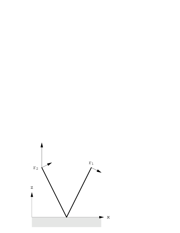
FIG. 2.: Illustration of the axial part of the correlation tensor: electric field created at ${\bf r}_{1}$ by a dipole located at ${\bf r}_{2}$ and oscillating perpendicular to the interface.

2 Connection with the damping rates of the excited state Zeeman sublevels

As shown in Ref. [41], the atomic internal relaxation processes associated with spontaneous emission close to a vacuum-dielectric interface can be entirely described by means of the damping rates $\Gamma_{\|}(z)$ and $\Gamma_{\bot}(z)$ of classical oscillating dipoles located at a distance $z$ above the dielectric medium, polarized parallel or orthogonal to the interface, respectively, and such that $\Gamma_{\|,\bot}(z\rightarrow\infty)=\Gamma_{\infty}$. More precisely, one shows that the contribution $\dot{\rho}_{ee,relax}$ of spontaneous emission to the evolution of the excited state part of the internal atomic density matrix for an atom at rest in ${\bf r}$ reads [41]

$$\dot{\rho}_{ee,relax}=$$ (72)

$$=-\frac{1}{2}\left\{\Gamma_{\|}(z)\,d_{x}^{+}d_{x}^{-}+\Gamma_{\|}(z)\,d_{y}^{+}d_{y}^{-}+\Gamma_{\bot}(z)\,d_{z}^{+}d_{z}^{-},\rho_{ee}\right\}$$ (73)

By comparing Eq.(72) with Eq.(16), which yields

$$\dot{\rho}_{ee,relax}=-\frac{\Gamma_{\infty}}{2}\left\{C^{i,j}({\bf r},{\bf r})\,d_{i}^{+}\,d_{j}^{-}\,,\rho_{ee}\right\}$$ (74)

one can readily deduce that

$$c_{\|}(z) = C^{x,x}(z;{\bf 0})=C^{y,y}(z;{\bf 0})=\frac{\Gamma_{\|}(z)}{\Gamma_{\infty}}=$$ (76)

$$= 1+c_{0}(z;0)-{\textstyle\frac{1}{3}}q_{0}(z;0)$$ (77)

$$c_{\perp}(z) = C^{z,z}(z;{\bf 0})=\frac{\Gamma_{\perp}(z)}{\Gamma_{\infty}}=$$ (78)

$$= 1+c_{0}(z;0)+{\textstyle\frac{2}{3}}q_{0}(z;0)$$ (79)

As can be checked on the expression of $c_{0}$ and $q_{0}$ [Eqs. (C52) and (C54)], these results are consistent with the well-known form of $\Gamma_{\|}(z)$ and $\Gamma_{\bot}(z)$ [28, 41].

3 Evanescent driving field

We focus in this paper on an evanescent driving laser field without polarization gradient, i.e., we consider the field profile

$$\mathchoice{{\hbox{\boldmath$\displaystyle\xi$}}}{{\hbox{\boldmath$\textstyle\xi$}}}{{\hbox{\boldmath$\scriptstyle\xi$}}}{{\hbox{\boldmath$\scriptscriptstyle\xi$}}}({\bf r})=\mathchoice{{\hbox{\boldmath$\displaystyle\xi$}}}{{\hbox{\boldmath$\textstyle\xi$}}}{{\hbox{\boldmath$\scriptstyle\xi$}}}{{\hbox{\boldmath$\scriptscriptstyle\xi$}}}_{0}\exp{(-\kappa}z{+}iQx{)}$$ (80)

where $Q^{2}-\kappa^{2}=k^{2}$ and $\mathchoice{{\hbox{\boldmath$\displaystyle\xi$}}}{{\hbox{\boldmath$\textstyle\xi$}}}{{\hbox{\boldmath$\scriptstyle\xi$}}}{{\hbox{\boldmath$\scriptscriptstyle\xi$}}}_{0}$ is a constant vector. This field is created by total internal reflection of a plane laser wave inside the dielectric (hence, $Q>k$). For the two elementary polarizations $TE$ and $TM$ of the incident wave, we have

$$\mathchoice{{\hbox{\boldmath$\displaystyle\xi$}}}{{\hbox{\boldmath$\textstyle\xi$}}}{{\hbox{\boldmath$\scriptstyle\xi$}}}{{\hbox{\boldmath$\scriptscriptstyle\xi$}}}_{0}^{(TE)}={\bf e}_{y},\qquad\mathchoice{{\hbox{\boldmath$\displaystyle\xi$}}}{{\hbox{\boldmath$\textstyle\xi$}}}{{\hbox{\boldmath$\scriptstyle\xi$}}}{{\hbox{\boldmath$\scriptscriptstyle\xi$}}}_{0}^{(TM)}=\frac{i\kappa\,{\bf e}_{x}-Q\,{\bf e}_{z}}{k}.$$ (81)

Note that in the $TM$-case, the polarization of the evanescent wave is elliptic: it approaches a linear polarization in the vicinity of the critical angle ($\kappa\to 0$) and a circular one ($\sigma^{-}$ with respect to the positive $y$-axis) far from the critical angle ($\kappa\simeq Q$).

B $J_{g}=0$$\to J_{e}=1$ atomic transition

In this subsection we consider the simple situation of a scalar atom (a $J_{g}=0\to J_{e}=1$ transition) and calculate the radiation pressure force and the momentum diffusion tensor. The Wigner function of the ground state is now a scalar, and the atomic dipole operators ${\bf b}^{\pm}({\bf r})$ [Eq.(22)] reduce to $c$-number functions that are simply given by the electric field profile

$${\bf b}^{-}({\bf r})=\mathchoice{{\hbox{\boldmath$\displaystyle\xi$}}}{{\hbox{\boldmath$\textstyle\xi$}}}{{\hbox{\boldmath$\scriptstyle\xi$}}}{{\hbox{\boldmath$\scriptscriptstyle\xi$}}}({\bf r}).$$ (82)

The advantage of such a transition is that it provides a good way to single out the effect of the interface on the basic atomic external dynamics, with the minimum complications introduced by the interface-modified internal atomic dynamics.

1 Fluorescence rate

The atomic ground state reducing to a single level, the only nontrivial feature of the optical pumping equation (46) is the total atomic fluorescence rate $\Gamma^{\prime}(z)$, that is given by the trace of either term of the right-hand side of Eq.(48). One thus finds

$$\Gamma^{\prime}(z)=\Gamma_{\infty}^{\prime}\left(c_{\|}(z)|\mathchoice{{\hbox{\boldmath$\displaystyle\xi$}}}{{\hbox{\boldmath$\textstyle\xi$}}}{{\hbox{\boldmath$\scriptstyle\xi$}}}{{\hbox{\boldmath$\scriptscriptstyle\xi$}}}_{0\|}|^{2}+c_{\perp}(z)|\xi_{0\bot}|^{2}\right)e^{-2\kappa z}$$ (83)

with $\mathchoice{{\hbox{\boldmath$\displaystyle\xi$}}}{{\hbox{\boldmath$\textstyle\xi$}}}{{\hbox{\boldmath$\scriptstyle\xi$}}}{{\hbox{\boldmath$\scriptscriptstyle\xi$}}}_{0}=(\mathchoice{{\hbox{\boldmath$\displaystyle\xi$}}}{{\hbox{\boldmath$\textstyle\xi$}}}{{\hbox{\boldmath$\scriptstyle\xi$}}}{{\hbox{\boldmath$\scriptscriptstyle\xi$}}}_{0\|},\xi_{0\bot})$. The influence of the interface on the internal ground state dynamics hence amounts to a different space-dependence of the broadening of the ground state level in addition to the one associated with the space dependence of the driving laser field. For comparison, the parenthesis in Eq.(83) is space independent in free space and equal to $|\mathchoice{{\hbox{\boldmath$\displaystyle\xi$}}}{{\hbox{\boldmath$\textstyle\xi$}}}{{\hbox{\boldmath$\scriptstyle\xi$}}}{{\hbox{\boldmath$\scriptscriptstyle\xi$}}}_{0}|^{2}$. It is also interesting to note that the fluorescence rate (83) involves the intensity of the ‘transverse’ ($|\xi_{0\bot}|^{2}$) and ‘longitudinal’ ($|\mathchoice{{\hbox{\boldmath$\displaystyle\xi$}}}{{\hbox{\boldmath$\textstyle\xi$}}}{{\hbox{\boldmath$\scriptstyle\xi$}}}{{\hbox{\boldmath$\scriptscriptstyle\xi$}}}_{0\|}|^{2}$) parts of the driving field independently, as a result from the rotational symmetry breaking due to the interface. As a consequence, the two elementary polarizations of the evanescent wave yield different spatial variations of the fluorescence rate:

$$\Gamma^{\prime(TE)}(z) = \Gamma_{\infty}^{\prime}\,c_{\|}(z)\,e^{-2\kappa z}$$ (85)

$$\Gamma^{\prime(TM)}(z) = \,\Gamma_{\infty}^{\prime}\,\frac{\kappa^{2}c_{\|}(z)+Q^{2}c_{\perp}(z)}{k^{2}}\,e^{-2\kappa z}$$ (86)

Hence, depending on the polarization of the driving evanescent wave, the atomic fluorescence permits to probe different combinations of the correlation tensor components $c_{\|}(z)$ and $c_{\perp}(z)$.

2 Radiation pressure force

By inserting the field correlation tensor (C32, C42) and the evanescent field profile (80) into the general results (53, 55), one readily finds that the departure contribution (55) to the radiation pressure vanishes for a scalar atom. After some algebra, the feeding term (53) yields the following result for the radiation pressure force

$${\bf F}^{(sp)}({\bf r}) = \Gamma^{\prime}(z)\,\hbar Q\,{\bf e}_{x}+$$ (88)

$$+2\Gamma_{\infty}^{\prime}\,\hbar k\,a_{1}(z;0)\,\text{Im}\,(\mathchoice{{\hbox{\boldmath$\displaystyle\xi$}}}{{\hbox{\boldmath$\textstyle\xi$}}}{{\hbox{\boldmath$\scriptstyle\xi$}}}{{\hbox{\boldmath$\scriptscriptstyle\xi$}}}_{0\|}\xi_{0\bot}^{*})\,e^{-2\kappa z}$$

The first term of the force (88) corresponds to the rule-of-the-thumb expression for the radiation pressure: it is the product of the fluorescence rate (83) and the photon momentum $\hbar Q$ carried by the evanescent wave along its propagation direction. The second term arises from the fact that the actual driving field consists of the sum of the incoming laser evanescent wave and of the reflected part of the field radiated by the atomic dipole. Because the radiation pressure force exerted on a $J_{g}=0\to J_{e}=1$ atom is proportional to the phase-gradient of the total driving field, it actually appears as the sum of a contribution proportional to the phase gradient of the evanescent incoming wave [first term of Eq.(88)] and of a term involving the phase gradient of the reflected dipole field [second term of Eq.(88)]. It is therefore not surprising to find that the reflected field contribution to the radiation pressure is proportional to the axial coefficient $a_{1}$ that, as previously discussed, is directly connected to field reflection processes at the interface.

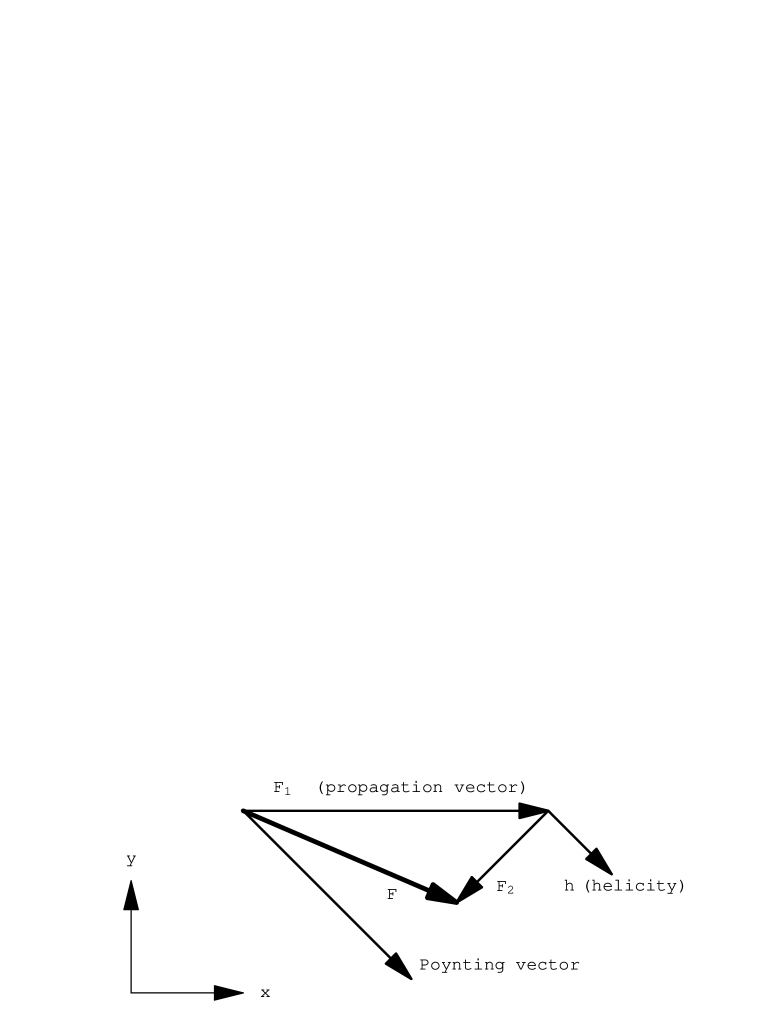
FIG. 3.: Illustration of the radiation pressure force in a circularly polarized evanescent wave.
F₁: usual radiation pressure (parallel to driving field’s propagation vector); F₂: correction due to partial field reflection at the dielectric surface; F: full force. The helicity vector h of the circular polarization and the Poynting vector of the evanescent wave (using the standard definition) are also shown.

For the $TE$ and $TM$ polarizations of the evanescent driving field, this correction to the radiation pressure force is difficult to observe: indeed, the vector $\text{Im}\,(\mathchoice{{\hbox{\boldmath$\displaystyle\xi$}}}{{\hbox{\boldmath$\textstyle\xi$}}}{{\hbox{\boldmath$\scriptstyle\xi$}}}{{\hbox{\boldmath$\scriptscriptstyle\xi$}}}_{0\|}\xi_{0\bot}^{*})$ vanishes in the $TE$-case and is parallel to ${\bf e}_{x}$ in the $TM$-case [cf. Eq.(81)], thus modifying slightly the magnitude of ${\bf F}^{(sp)}$. A more prominent modification occurs for a generic combination of $TE$ and $TM$ polarizations. The effect is actually maximum for a circular polarization of the evanescent wave in a plane perpendicular to the interface, which can be achieved for

$$\mathchoice{{\hbox{\boldmath$\displaystyle\xi$}}}{{\hbox{\boldmath$\textstyle\xi$}}}{{\hbox{\boldmath$\scriptstyle\xi$}}}{{\hbox{\boldmath$\scriptscriptstyle\xi$}}}_{0}^{(\sigma)}=\mathchoice{{\hbox{\boldmath$\displaystyle\xi$}}}{{\hbox{\boldmath$\textstyle\xi$}}}{{\hbox{\boldmath$\scriptstyle\xi$}}}{{\hbox{\boldmath$\scriptscriptstyle\xi$}}}_{0}^{(TM)}+i\mathchoice{{\hbox{\boldmath$\displaystyle\xi$}}}{{\hbox{\boldmath$\textstyle\xi$}}}{{\hbox{\boldmath$\scriptstyle\xi$}}}{{\hbox{\boldmath$\scriptscriptstyle\xi$}}}_{0}^{(TE)}.$$ (89)

The field’s polarization is then $\sigma^{+}$ with respect to an axis parallel to the interface (given by the ‘helicity’ vector ${\bf h}=(2Q/k)[{\bf e}_{x}-(\kappa/k){\bf e}_{y}]$, cf. Fig. 3). The total fluorescence rate is given by

$$\Gamma^{\prime(\sigma)}(z)=\Gamma_{\infty}^{\prime}\,\frac{Q^{2}}{k^{2}}\,\left(c_{\|}(z)+c_{\perp}(z)\right)\,e^{-2\kappa z}$$ (90)

and the reflected field contribution to the radiation pressure force is found perpendicular to the helicity ${\bf h}$, yielding

$${\bf F}^{(sp)}(z) = \hbar Q\Gamma^{\prime(\sigma)}(z){\bf e}_{x}$$ (92)

$$-2\hbar Q\Gamma_{\infty}^{\prime}\,a_{1}(z;0)\,e^{-2\kappa z}\left(\frac{\kappa}{k}{\bf e}_{x}+{\bf e}_{y}\right).$$

Thus, the radiation pressure force forms a nonzero, $z\,$-dependent angle with the evanescent wave propagation vector $Q\,{\bf e}_{x}$. This is represented in Fig. 4 where the angle and magnitude of the radiation pressure force (92) are plotted as a function of the distance $z$ from the dielectric surface.

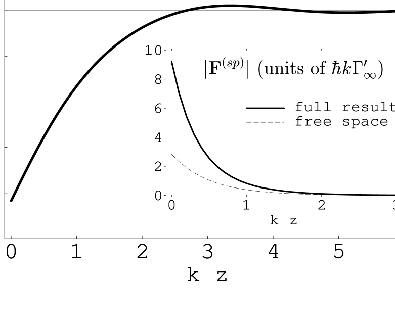
FIG. 4.: Direction of the radiation pressure force in a circularly polarized evanescent wave, as a function of distance from the dielectric. The curve shows the angle between the actual force and the evanescent wave’s propagation vector (the vectors F and F₁ of Fig. 3). For these parameters, the field’s Poynting vector forms an angle of $-45^{\circ}$ with the propagation vector F₁. The inset gives the magnitude of the force, using either the exact result (92) (full line) or ignoring both the increased fluorescence rate and the force correction F₂ (dashed line).
Parameters: refractive index $n_{0}=1.5$, evanescent driving field with $\kappa=k$, $Q=\sqrt{2}\,k$. The force is plotted is units of $\hbar k\Gamma^{\prime}_{\infty}$, as a function of $kz$.

We finally note that a related effect was discussed by Roosen and Imbert [43]: these authors pointed out that the Poynting vector of an evanescent wave is not parallel to its propagation vector if the wave is circularly polarized. If one assumes the radiation pressure force to be parallel to the Poynting vector of the driving field, which seems tempting because the Poynting vector represents the local momentum of the field, one thus finds a result reminding of (92). In fact, it is well-known that this assumption is not correct, as can be readily checked on the simple example of a $J_{g}=0\to J_{e}=1$ atom interacting in free space with two plane waves

$$\mathchoice{{\hbox{\boldmath$\displaystyle\xi$}}}{{\hbox{\boldmath$\textstyle\xi$}}}{{\hbox{\boldmath$\scriptstyle\xi$}}}{{\hbox{\boldmath$\scriptscriptstyle\xi$}}}({\bf r})=e^{ikx}{\bf e}_{z}+e^{iky}{\bf e}_{x}$$ (93)

leading to a Poynting vector

$${\bf\Pi}\propto{\bf e}_{x}+{\bf e}_{y}-\cos\left[k(x-y)\right]\,{\bf e}_{z}$$ (94)

whereas the radiation pressure force is clearly oriented along ${\bf e}_{x}+{\bf e}_{y}$. This problem can be readily solved by noticing that the Poynting vector ${\bf\Pi}$ is only defined up to a curl, as shown by the continuity equation

$${\bf\nabla.\Pi+\partial}_{t}\varepsilon=0$$ (95)

where $\varepsilon$ is the electromagnetic energy density. It is thus straightforward to show that it is always possible to define a “novel” Poynting vector satisfying the continuity equation and being parallel to the radiation pressure force.

3 Momentum diffusion tensor

The momentum diffusion tensor can be readily obtained from Eq.(60) using the field correlations (C32, C42) and replacing the dipole operators ${\bf b}^{\pm}({\bf r})$ by the evanescent field profile according to Eq.(80). One thus finds

$$D^{k,l}(z)=\frac{\hbar^{2}}{8}\frac{\partial^{2}\Gamma^{\prime}(z)}{\partial z^{2}}\,\delta^{k,z}\delta^{l,z}\,-\,\frac{\hbar^{2}\Gamma_{\infty}^{\prime}}{2}\frac{\partial^{2}{\cal A}}{\partial s_{k}\partial s_{l}}(z;{\bf 0})$$ (96)

where

$${\cal A}(z;{\bf s})=C^{i,j}(z;{\bf s})\,\xi_{0i}^{*}\,\xi_{0j}\,\exp(-2\kappa z+iQ\,{\bf s.e}_{x})$$ (97)

We now discuss the physical significance of Eq.(96) in more details, with an emphasis on the influence of the interface on momentum diffusion. We start by considering the first term on the right-hand side of Eq.(96), that corresponds to $D_{\text{depart}}^{k,l}$ [see Eq.(61)]. In order to single out the interface contribution, it is convenient to write the total fluorescence rate in the form

$$\Gamma^{\prime}(z)=\Gamma_{\infty}^{\prime}\left|\mathchoice{{\hbox{\boldmath$\displaystyle\xi$}}}{{\hbox{\boldmath$\textstyle\xi$}}}{{\hbox{\boldmath$\scriptstyle\xi$}}}{{\hbox{\boldmath$\scriptscriptstyle\xi$}}}_{0}\right|^{2}\,e^{-2\kappa z}+\Gamma_{int}^{\prime}(z)$$ (98)

yielding two contributions to $D_{\text{depart}}^{z,z}$

$$D_{\text{depart}}^{z,z}(z)=\frac{\hbar^{2}\kappa^{2}\Gamma_{\infty}^{\prime}\left|\mathchoice{{\hbox{\boldmath$\displaystyle\xi$}}}{{\hbox{\boldmath$\textstyle\xi$}}}{{\hbox{\boldmath$\scriptstyle\xi$}}}{{\hbox{\boldmath$\scriptscriptstyle\xi$}}}_{0}\right|^{2}}{2}\,e^{-2\kappa z}+\frac{\hbar^{2}}{8}\frac{\partial^{2}\Gamma_{int}^{\prime}(z)}{\partial z^{2}}$$ (99)

The first term on the right-hand side of Eq.(99) does not involve any surface-induced effects (apart from the existence of the evanescent driving field) and is associated with the shrinking of the atomic spatial coherence (hence a broadening in momentum space) due to the non-uniform, exponential photon absorption probability. This corresponds to the intuitive fact that the coherence of an atomic wavepacket incident on an evanescent wave mirror will be destroyed more efficiently by absorption-spontaneous emission cycles close to the interface than far away as a result of the inhomogeneous laser intensity. The second term of Eq.(99) is a correction to $D_{\text{depart}}^{z,z}$ arising from the modification of the fluorescence rate by the interface, that is responsible for an additional spatial modulation of the photon absorption probability, hence an additional cause for momentum diffusion. As is well-known, the dipole damping rates $\Gamma_{\|}(z)$ and $\Gamma_{\bot}(z)$ display an exponential dependence close to the interface, and then tend toward their asymptotic value $\Gamma_{\infty}$ with some damped oscillations [41]. $\Gamma_{int}^{\prime}(z)$, and consequently $D_{\text{depart}}^{z,z}$, are therefore expected to exhibit the same kind of behaviour [see Eqs. (83) and (99)].

Consider now the second term on the right-hand side of Eq.(96), corresponding to $D_{\text{feed}}^{k,l}$ [see Eq.(62)]. Again, the influence of the interface can be sorted out by expressing ${\cal A}$ in the form

$${\cal A}(z;{\bf s)} = {\cal A}_{\infty}(z;{\bf s})+{\cal A}_{int}(z;{\bf s}_{\|})$$ (100)

$${\cal A}_{\infty}(z;{\bf s}) = C_{\infty}^{i,j}({\bf s})\,\xi_{0i}^{*}\,\xi_{0j}\,\exp(-2\kappa z+iQ\,{\bf s.e}_{x})$$ (101)

$${\cal A}_{int}(z;{\bf s}_{\|}) = C_{int}^{i,j}(z;{\bf s}_{\|})\,\xi_{0i}^{*}\,\xi_{0j}\,\exp(-2\kappa z+iQ\,{\bf s.e}_{x})$$ (102)

Because ${\cal A}_{\infty}$ only involves the free-space correlation tensor $C_{\infty}^{i,j}$, its contribution to $D_{\text{feed}}^{k,l}$ is analogous to that usually encountered in free space for any driving laser field, i.e., it accounts for the random walk of the atoms in momentum space due to their recoil during spontaneous emission of photons, the spontaneous emission diagram being assumed as in free space. The contribution of ${\cal A}_{int}$ to momentum diffusion, involving the complex nonlocal correlations between the vacuum field components induced by the interface, exhibits an interesting feature. Because ${\cal A}_{int}$ is independent of the $z$-component of the relative position ${\bf s}$ (because such is $C_{int}^{i,j}$), the interface-induced modifications of momentum diffusion due to changes in spontaneous emission in the vicinity of the dielectric medium will only take place parallel to the interface, a result that is not obvious when considering the important modifications of the spontaneous emission diagrams due to the interface [41].

FIG. 5.: Momentum diffusion coefficient for a scalar atom driven by a $TE$ [(a)] and a $TM$ [(b)] polarized evanescent wave. Thick solid line: trace $D(z)$ (103) of the diffusion tensor; dashed line: lateral diffusion coefficient $D_{\|}(z)=D_{xx}(z)+D_{yy}(z)$; dotted line: diffusion coefficient $D_{zz}(z)$ perpendicular to the interface; thin solid line: trace $D(z)$ of the diffusion tensor in free space (both the modified vacuum correlations and the curvature of the driving field are neglected).
Parameters: same as Fig. 4. The diffusion coefficient is plotted in units of $\hbar^{2}k^{2}\Gamma^{\prime}_{\infty}$, as a function of $kz$.

Quantitative results for the momentum diffusion tensor are displayed in Figs. 5–6. In Fig. 5 is plotted the trace of the diffusion tensor

$$D(z)=\sum_{i}D^{i,i}(z)$$ (103)

that permits to estimate the total width $\Delta p$ of the atomic momentum distribution: for a spatially constant diffusion coefficient,

$$\Delta p^{2}\simeq 2Dt$$ (104)

which may be generalized to

$$\Delta p^{2}\simeq 2\int\!dt\,D[\langle z(t)\rangle]$$ (105)

where $\langle z(t)\rangle$ is the mean atomic trajectory in the evanescent field’s dipole potential. Eq.(105) is valid provided the momentum diffusion is sufficiently small so that individual atomic trajectories remain close to the mean path, an assumption that may become questionable depending on the experimental conditions. The integral (105) may be estimated from the typical timescale $\tau\simeq 2M/\kappa p_{z,inc}$ for the reflection [52, 53] ($-p_{z,inc}$: incident atomic momentum along $z$) and the position $z_{0}$ of the turning point of the mean path: $\Delta p^{2}\simeq 2\tau D(z_{0})$. The diffusion coefficients plotted in Fig. 5 may thus be viewed as the squared momentum width of the reflected atoms, given the interaction time and varying the distance $z=z_{0}$ of the turning point.

From Fig. 5, we observe that the atomic momentum diffusion perpendicular to the surface (the coefficient $D^{z,z}$ represented by the dotted curve) is, on its own, comparable to the diffusion in free space (the thin solid curve, neglecting the curvature of the exponential fluorescence rate and the modified vacuum correlations). This may be compared with Fig. 6 where the evanescent driving field has a large decay length $1/\kappa$ (total internal reflection close to the critical angle). The exponential field profile is then essentially constant and the perpendicular momentum diffusion decreases. In this direction, the momentum diffusion coefficient $D^{z,z}$ is now determined, on the one hand, by the spontaneous photons’ recoil, $D^{z,z}_{\text{feed}}$, and, on the other hand, by the derivatives of the fluorescence rates $\Gamma_{\|,\perp}(z)$ that enter into $D^{z,z}_{\text{depart}}$ (99). Also, for the long-range evanescent wave, the $TE$ and $TM$ polarizations produce a similar momentum diffusion since they both correspond to a (nearly) linearly polarized driving field.

FIG. 6.: Same as Fig. 5, but for an evanescent driving field with larger decay length: $\kappa=0.1\,k$, $Q\approx 1.005\,k$.

In conclusion, we observe that the momentum diffusion tensor is systematically larger close to the dielectric surface compared to free space (the thin solid lines in Figs. 5, 6), by a factor of about three to four. Translating the width of the atomic momentum distribution into a coherence length, we see that close to the surface, spontaneous emission destroys the atomic coherence more efficiently than expected from free-space considerations. This may have been expected from the enhanced fluorescence rates $\Gamma_{\|,\perp}(z)$ compared to $\Gamma_{\infty}$, as well as from the spatial subwavelength structure of both the evanescent field and the vacuum field correlations. Finally, we note that this diffusion tensor also translates into an increased temperature limit for radiative atom traps in the vicinity of surfaces [19, 20, 21, 22, 23, 24, 25].

C $J_{g}=1/2$ atom

In this section, we turn to a second application of the theory developed in Sec. II and focus on the optical pumping processes taking place in atoms having a nontrivial Zeeman sublevel structure in their ground state. By considering the simple case of a $J_{g}=1/2$ atom, we show that these processes are modified both quantitatively and qualitatively in the vicinity of the dielectric interface: since the fluorescence rates depend on both the atom-interface distance and the atomic dipole orientation, the optical pumping rates are modified. More strikingly, a net ground-state magnetization is predicted to occur in a linearly polarized driving field if the atomic recoil is taken into account. We illustrate this effect by an explicit calculation of the radiation pressure force.

1 Atomic magnetization variables

In the case of a $J_{g}=1/2$ atom, the Wigner function $W({\bf r},{\bf p})$ takes the form of a hermitian $2\times 2$ matrix describing the populations and Zeeman coherences of the ground state. It is convenient to represent this matrix using the vector $\mathchoice{{\hbox{\boldmath$\displaystyle\sigma$}}}{{\hbox{\boldmath$\textstyle\sigma$}}}{{\hbox{\boldmath$\scriptstyle\sigma$}}}{{\hbox{\boldmath$\scriptscriptstyle\sigma$}}}=(\sigma_{x},\sigma_{y},\sigma_{z})$ of Pauli matrices

$$W={\textstyle\frac{1}{2}}\left(w+\mathchoice{{\hbox{\boldmath$\displaystyle\sigma$}}}{{\hbox{\boldmath$\textstyle\sigma$}}}{{\hbox{\boldmath$\scriptstyle\sigma$}}}{{\hbox{\boldmath$\scriptscriptstyle\sigma$}}}\cdot{\bf J}\right)$$ (106)

With this definition, the scalar function $w({\bf r},{\bf p})$ describes the phase-space distribution of the total population, whereas the real vector ${\bf J}({\bf r},{\bf p})$ (analogous to the Bloch vector for a two-level atom) gives the phase-space distribution of the atomic magnetization: for unpolarized atoms, e.g., one has ${\bf J}\equiv{\bf 0}$; for an ensemble of atoms prepared in the sublevel $|+1/2\rangle_{z}$ with respect to the $z$ axis, e.g., $J_{z}({\bf r},{\bf p})=w({\bf r},{\bf p})$ and $J_{x,y}\equiv 0$. The evolution equations for the total population and the magnetization vector are obtained from the G.O.B.E. by taking the appropriate traces:

$$w({\bf r},{\bf p}) = \text{Tr}\,W({\bf r},{\bf p}),$$ (108)

$${\bf J}({\bf r},{\bf p}) = \text{Tr}\,[\mathchoice{{\hbox{\boldmath$\displaystyle\sigma$}}}{{\hbox{\boldmath$\textstyle\sigma$}}}{{\hbox{\boldmath$\scriptstyle\sigma$}}}{{\hbox{\boldmath$\scriptscriptstyle\sigma$}}}W({\bf r},{\bf p})].$$ (109)

We next need the action of the reduced dipole operators ${\bf b}^{\pm}({\bf r})$ on the Wigner matrix. From the Clebsch–Gordan coefficients for the $J_{g}=1/2\to J_{e}=J_{g},J_{g}+1$ transitions, one finds

$${\bf b}^{-}({\bf r}) = \beta\,\mathchoice{{\hbox{\boldmath$\displaystyle\xi$}}}{{\hbox{\boldmath$\textstyle\xi$}}}{{\hbox{\boldmath$\scriptstyle\xi$}}}{{\hbox{\boldmath$\scriptscriptstyle\xi$}}}({\bf r})+i\alpha\,\mathchoice{{\hbox{\boldmath$\displaystyle\sigma$}}}{{\hbox{\boldmath$\textstyle\sigma$}}}{{\hbox{\boldmath$\scriptstyle\sigma$}}}{{\hbox{\boldmath$\scriptscriptstyle\sigma$}}}\times\mathchoice{{\hbox{\boldmath$\displaystyle\xi$}}}{{\hbox{\boldmath$\textstyle\xi$}}}{{\hbox{\boldmath$\scriptstyle\xi$}}}{{\hbox{\boldmath$\scriptscriptstyle\xi$}}}({\bf r}),$$ (113)

$$\begin{array}[]{l}J_{e}=1/2:\qquad\beta=1/3,\quad\alpha=-1/3,\\ J_{e}=3/2:\qquad\beta=2/3,\quad\alpha=1/3;\end{array}$$

while ${\bf b}^{+}({\bf r})$ is given by the hermitian conjugate. The first term $\beta\,\mathchoice{{\hbox{\boldmath$\displaystyle\xi$}}}{{\hbox{\boldmath$\textstyle\xi$}}}{{\hbox{\boldmath$\scriptstyle\xi$}}}{{\hbox{\boldmath$\scriptscriptstyle\xi$}}}({\bf r})$ in Eq.(113) is similar to the reduced dipole operator for a scalar atom (it is parallel to the driving field’s polarization vector $\mathchoice{{\hbox{\boldmath$\displaystyle\xi$}}}{{\hbox{\boldmath$\textstyle\xi$}}}{{\hbox{\boldmath$\scriptstyle\xi$}}}{{\hbox{\boldmath$\scriptscriptstyle\xi$}}}({\bf r})$); the second term $i\alpha\,\mathchoice{{\hbox{\boldmath$\displaystyle\sigma$}}}{{\hbox{\boldmath$\textstyle\sigma$}}}{{\hbox{\boldmath$\scriptstyle\sigma$}}}{{\hbox{\boldmath$\scriptscriptstyle\sigma$}}}\times\mathchoice{{\hbox{\boldmath$\displaystyle\xi$}}}{{\hbox{\boldmath$\textstyle\xi$}}}{{\hbox{\boldmath$\scriptstyle\xi$}}}{{\hbox{\boldmath$\scriptscriptstyle\xi$}}}({\bf r})$ accounts for couplings between the ground-state Zeeman sublevels, and therefore describes specific multilevel effects such as Raman couplings.

2 Internal dynamics

As in the scalar atom situation, we start our analysis by considering the classical optical pumping equation (46) accounting for the internal atomic dynamics. In the $J_{g}=1/2$ case, two quantities characterize the internal atomic dynamics: the ground state light shifts [Eq.(30)] and the optical pumping rates [Eq.(48)] (we do not consider in this section the energy level shifts induced by the interface). We discuss in some detail the case of a circularly polarized evanescent wave and calculate the pumping rate.

a General.

Let us first write down the light-shift Hamiltonian (30) (also a hermitian $2\times 2$ matrix):

$$H_{eff} = \hbar\Delta^{\prime}\,e^{-2\kappa z}\,{\bf b}_{0}^{+}\cdot\mathchoice{{\hbox{\boldmath$\displaystyle\xi$}}}{{\hbox{\boldmath$\textstyle\xi$}}}{{\hbox{\boldmath$\scriptstyle\xi$}}}{{\hbox{\boldmath$\scriptscriptstyle\xi$}}}_{0}$$ (115)

$$= \hbar\Delta^{\prime}\,e^{-2\kappa z}\,(\beta|\mathchoice{{\hbox{\boldmath$\displaystyle\xi$}}}{{\hbox{\boldmath$\textstyle\xi$}}}{{\hbox{\boldmath$\scriptstyle\xi$}}}{{\hbox{\boldmath$\scriptscriptstyle\xi$}}}_{0}|^{2}+\alpha{\bf h}\cdot\mathchoice{{\hbox{\boldmath$\displaystyle\sigma$}}}{{\hbox{\boldmath$\textstyle\sigma$}}}{{\hbox{\boldmath$\scriptstyle\sigma$}}}{{\hbox{\boldmath$\scriptscriptstyle\sigma$}}})$$ (116)

$${\bf h} = \text{Im}\,\mathchoice{{\hbox{\boldmath$\displaystyle\xi$}}}{{\hbox{\boldmath$\textstyle\xi$}}}{{\hbox{\boldmath$\scriptstyle\xi$}}}{{\hbox{\boldmath$\scriptscriptstyle\xi$}}}_{0}^{*}\times\mathchoice{{\hbox{\boldmath$\displaystyle\xi$}}}{{\hbox{\boldmath$\textstyle\xi$}}}{{\hbox{\boldmath$\scriptstyle\xi$}}}{{\hbox{\boldmath$\scriptscriptstyle\xi$}}}_{0}$$ (117)

where ${\bf b}_{0}^{\pm}$ is given by Eq.(113), replacing $\mathchoice{{\hbox{\boldmath$\displaystyle\xi$}}}{{\hbox{\boldmath$\textstyle\xi$}}}{{\hbox{\boldmath$\scriptstyle\xi$}}}{{\hbox{\boldmath$\scriptscriptstyle\xi$}}}({\bf r})$ with $\mathchoice{{\hbox{\boldmath$\displaystyle\xi$}}}{{\hbox{\boldmath$\textstyle\xi$}}}{{\hbox{\boldmath$\scriptstyle\xi$}}}{{\hbox{\boldmath$\scriptscriptstyle\xi$}}}_{0}$, and where the ${\bf h}$ vector corresponds to the helicity of the driving field. Following Cohen-Tannoudji and Dupont-Roc [54], one may interpret the second term of the light-shift operator (a) in terms of a fictitious magnetic field parallel to the helicity ${\bf h}$. This interpretation is supported by the equation of motion for the atomic magnetization vector ${\bf J}$: it is obtained using Eq.(48) for the Wigner matrix $W$ that takes the following form

$$\left.\dot{W}_{relax}\right|_{0} = \Gamma_{\infty}^{\prime}\,e^{-2\kappa z}\,C^{i,i}(z;{\bf 0})\Big{(}b_{0i}^{-}Wb_{0i}^{+}$$ (119)

$$\quad-{\textstyle\frac{1}{2}}\{b_{0i}^{+}b_{0i}^{-},\,W\}\Big{)}$$

After some straightforward algebra with the Pauli matrices, we find from the light-shift Hamiltonian (a) and Eq.(119) the following equation of motion

$$\left.\frac{\partial{\bf J}}{\partial t}\right|_{0}=2\alpha\,\Delta^{\prime}e^{-2\kappa z}\,{\bf h}\times{\bf J}+2\alpha^{2}\Gamma_{\infty}^{\prime}\,e^{-2\kappa z}\,{\cal C}(z){\bf h}$$ (121)

$$-\,2\alpha^{2}\Gamma_{\infty}^{\prime}\,e^{-2\kappa z}\,\Big{(}(\text{Tr}\,{\cal F})\,{\cal C}(z){\bf J}+(\text{Tr}\,{\cal C}(z))\,{\cal F}{\bf J}\Big{)}$$ (122)

$$+\,2\Gamma_{\infty}^{\prime}\,e^{-2\kappa z}\Big{(}\alpha^{2}\{{\cal C}(z),\,{\cal F}\}{\bf J}-\alpha\beta[{\cal C}(z),\,{\cal F}]{\bf J}\Big{)}$$ (123)

We have used the following tensors

$$({\cal C}(z))^{i,j} = C^{i,j}(z;{\bf 0})=\left(\begin{array}[]{lll}c_{\|}(z)&0&0\\ 0&c_{\|}(z)&0\\ 0&0&c_{\bot}(z)\end{array}\right)_{x,y,z}$$ (127)

$$({\cal F})^{i,j} = \text{Re}\,\xi_{0i}^{*}\xi_{0j}$$ (128)

Since the total population $w={\rm Tr}\,W$ is conserved by optical pumping, we have put $w=1$ in Eq.(123).

In the equation of motion (123), one identifies the precession of the magnetization vector ${\bf J}$ around the effective magnetic field vector ${\bf h}$ (the first term) and the feeding of the magnetization ${\bf J}$ through optical pumping (the second term). The third and fourth terms describe the damping of the atomic magnetization through absorption-spontaneous emission cycles. The effect of the dielectric interface is encoded in the (diagonal) tensor ${\cal C}(z)$ whose elements are proportional to the dipole damping rates $\Gamma_{\|}$ and $\Gamma_{\bot}$ [see Eq.(74)]. It is interesting to note from Eq.(a) that optical pumping creates a magnetization aligned parallel to the vector ${\cal C}(z){\bf h}$ that is generally not parallel to the helicity ${\bf h}$ as a consequence of the anisotropic fluorescence rates. For the pumping process close to the dielectric interface, the one-point correlation tensor ${\cal C}(z)$ hence plays the role of an (anisotropic) ‘effective magnetic susceptibility’, linking the induced atomic magnetization to the effective magnetic field.

b Discussion of elementary polarizations.

According to the light-shift operator (116) and the equation of motion (123), the optical pumping process is characterized by the helicity vector ${\bf h}$ of the driving field. For the elementary polarizations of the evanescent wave, it becomes

$$\text{$TE$ polarization:}\quad{\bf h}^{(TE)} = {\bf 0}$$ (130)

$$\text{$TM$ polarization:}\quad{\bf h}^{(TM)} = -(2\kappa Q/k^{2}){\bf e}_{y}$$ (131)

We also mention for later use the case of a circularly polarized evanescent wave. As discussed at the end of Subsec. III B 2, the field’s polarization vector is given by Eq.(89) and one has

$$\text{circular polarization:}\quad{\bf h}^{(\sigma)}=(2Q/k)[{\bf e}_{x}-(\kappa/k){\bf e}_{y}]$$ (132)

In the $TE$ case, the helicity vanishes and hence no net magnetization builds up. The light-shifts for the two ground state Zeeman sublevels being identical (for the same reason), one would expect this case to yield a situation similar to the scalar atom of Subsec. III B. We shall see, however, that this is no longer true when the atomic recoil is taken into account (cf. Subsec. III C 3).

In the cases of $TM$ and circular polarization, the helicity is nonzero and optical pumping leads to a net atomic magnetization. In steady state, it aligns parallel to the $y$-axis in the $TM$ case, and parallel to an axis in the $xy$-plane for a circularly polarized evanescent wave. In both cases, the light-shift operator is diagonal with respect to these axis’, and the anisotropic magnetic susceptibility does not come into play. [This would be the case for a different relative phase between the $TE$ and $TM$ polarizations in Eq.(89), giving the helicity vector a nonzero component $h_{z}$.]

c Example: circular polarization.

As an example, we study in more detail the case of a circularly polarized evanescent wave and defer the $TM$ case to Appendix D.

FIG. 7.: Illustration of the fluorescence cycles for a $J=1/2\to J_{e}=3/2$ atom driven by (a) a linearly polarized field ($TE$ polarization); (b) a circularly polarized field (combination of $TE$ and $TM$ polarization); (c) a $TM$ polarized field (elliptic polarization).
For clarity, only the fluorescence cycles starting from the sublevel $|-1/2\rangle$ are shown. Note that these sublevels are defined with respect to a quantization axis that, in case (b), differs from cases (a) and (c).

It is convenient to introduce a rotated coordinate system with the ${\bf e}_{x^{\prime}}$ unit vector being parallel to the helicity (132). Choosing this as the quantization axis diagonalizes in fact the light-shift operator (a). From the magnetization’s evolution Eq.(a), it may also be verified that the components $J_{y^{\prime}},J_{z}$ decouple from $J_{x^{\prime}}$. If we assume that the atoms are initially unpolarized, the pumping process only depends on $J_{x^{\prime}}$ whose evolution is given by

$$\frac{\partial J_{x^{\prime}}}{\partial t}=\Gamma_{p}(z)[1-J_{x^{\prime}}]$$ (134)

where the ‘optical pumping rate’ equals

$$\Gamma_{p}(z)=4\alpha^{2}\frac{Q^{2}}{k^{2}}\Gamma^{\prime}_{\infty}e^{-2\kappa z}c_{\|}(z)$$ (135)

The significance of this equation becomes evident if we write down the evolution of the populations $w_{\pm}\equiv\frac{1}{2}(1\pm J_{x^{\prime}})$ of the Zeeman sublevels $|\pm 1/2\rangle_{x^{\prime}}$ with respect to the quantization axis. The following rate equations are easily found

$$\frac{\partial w_{+}}{\partial t}=\Gamma_{p}(z)w_{-},\qquad\frac{\partial w_{-}}{\partial t}=-\Gamma_{p}(z)w_{-}$$ (136)

and we see that the pumping rate $\Gamma_{p}(z)$ governs the transition $|-1/2\rangle_{x^{\prime}}\to|+1/2\rangle_{x^{\prime}}$ between the Zeeman sublevels. In this transition, the atom absorbs a $\sigma^{+}$ polarized photon (with respect to the $x^{\prime}$ axis) from the driving field and spontaneously emits a $\pi$ polarized photon (cf. Fig. 7b). The reverse transition is impossible since the driving field’s polarization is purely $\sigma^{+}$. From this elementary picture, we may understand why the optical pumping rate (135) involves the coefficient $c_{\|}$ from the vacuum correlation tensor: the spontaneous $\pi$ photon has in fact an electric field parallel to the $x^{\prime}$ axis, and its emission rate is proportional to the strength of the vacuum fluctuations polarized along this axis, hence proportional to the element $C^{x^{\prime},x^{\prime}}=c_{\|}$ of the correlation tensor.

The rate equations (136) show that in steady-state, the atoms are completely magnetized along the helicity vector of the driving field (the $x^{\prime}$ axis). With respect to optical pumping in free space, the only difference is hence the nonzero angle between this vector and the evanescent wave’s propagation vector $Q{\bf e}_{x}$.

A more detailed investigation of the pumping process may be done in the transient regime where the interaction time $\tau$ is smaller than the pumping time $1/\Gamma_{p}$. This regime is in fact typical for atomic mirror experiments where one seeks to avoid spontaneous emission because it reduces the coherence of the reflection. An approximate solution of Eq.(7) in the transient regime is (for initially unpolarized atoms)

$$\Gamma_{p}\tau\ll 1:\qquad J_{x^{\prime}} = w_{+}-w_{-}\simeq\Gamma_{p}(z_{0})\tau$$ (137)

$$\simeq 4\alpha^{2}\frac{Q^{2}}{k^{2}}\Gamma^{\prime}_{\infty}e^{-2\kappa z_{0}}c_{\|}(z_{0})\tau$$ (138)

The population difference now depends on the coefficient $c_{\|}(z_{0})$ at roughly the distance of closest approach $z_{0}$. The estimate (138) is actually very crude, since it neglects the fact that the sublevels $|\pm 1/2\rangle_{x^{\prime}}$ are subject to different light shift potentials in the circular polarization case. This leads to a different potential (and, ultimately, kinetic) energy after the sublevel change—a feature that has been studied already for both spontaneous [13, 15, 16] and stimulated [55, 56, 57] transitions between sublevels. In order to describe both the center-of-mass motion and the anisotropic vacuum correlations, one may use the full Fokker–Planck equation derived in Sec. II. An example of the corresponding ‘recoil-induced magnetizations’ is given in the next subsection.

For the sake of completeness, we have analyzed in Appendix D the optical pumping in a $TM$-polarized evanescent wave. In this case, the atoms do not become completely magnetized because the driving field [Eq.(81)] is elliptically polarized. [It contains both $\sigma^{+}$ and $\sigma^{-}$ components with respect to the $y$-axis, cf. Fig. 7c.] We find a steady-state magnetization $J_{y}^{(stat)}=-2\kappa Q/(\kappa^{2}+Q^{2})>-1$, and a pumping rate that is again proportional to the coefficient $c_{\|}$.

Summarizing, if atomic recoil is neglected, the internal dynamics close to the dielectric is subject to the following modifications as compared to free space. The optical pumping rates increase and differ according to the polarization of the spontaneous photon emitted in the pumping cycle. In a circularly polarized, evanescent driving field, a net atomic magnetization builds up that does not align parallel to the field propagation vector for two reasons: first, the magnetization is determined by the field helicity that is not parallel to its wave vector, and second, atomic magnetization and field helicity are connected by an anisotropic effective susceptibility because of the anisotropic fluorescence rates.

3 External dynamics: recoil-induced magnetization

We now consider the G.O.B.E. accounting for the atomic recoils during absorption and emission of photons. Among the huge diversity of non standard effects expected in the external dynamics of multilevel atoms in the vicinity of a vacuum-dielectric interface, that could not be addressed in a single paper, we focus here on radiation pressure and show that this force may induce a net magnetization of the atomic ground state for certain classes of the atomic velocity in a situation where the classical optical Bloch equations would predict a zero result (linearly polarized driving field).

a Radiation pressure force.

Consider the situation of a $J_{g}=1/2$ atom driven by a $TE$ polarized evanescent wave. Using the general expressions (53, 55) for the radiation pressure force, after a straightforward calculation using the Pauli matrices, one finds that the departure contribution ${\bf F}_{\text{depart}}^{(sp)}$ (55) vanishes, whereas the feeding contribution ${\bf F}_{\text{feed}}^{(sp)}$ (53) is a sum of two terms analogous to the ones encountered for the scalar atom [Eq.(88)]. The first of these contributions, ${\bf F}_{(1)}^{(sp)}$, corresponds to the product of the fluorescence rate and the evanescent field phase gradient. This force is hence parallel to the evanescent wave propagation vector $Q{\bf e}_{x}$. We find that this term does not couple the population $w$ and the magnetization components ${\bf J}$. The second contribution to the radiation pressure operator (53), ${\bf F}_{(2)}^{(sp)}$, is associated with the gradient of the field emitted by the atomic dipole and backreflected towards the atom by the dielectric interface, and involves the axial part of the field correlation tensor. This contribution, that vanished for a $TE$ polarization and a $J_{g}=0\rightarrow J_{e}=1$ atom, takes a nonzero value in the present situation and gives rise to a magnetization–population coupling. We interpret this coupling in terms of generalized rate equations for the Zeeman sublevel phase-space distributions.

To be more explicit, the contribution ${\bf F}_{(1)}^{(sp)}$ to the radiation pressure force appears in the following way in the Liouville equation for the magnetization component $J_{i}$ [cf. Eqs.(49, 109)]:

$$\text{Tr}\,\{\sigma_{i}\,{\bf F}^{(sp)}_{(1)}({\bf r})\cdot\nabla_{\bf p}W\}={\bf F}^{(sp)}_{(1)}({\bf r};J_{i})\cdot\nabla_{\bf p}J_{i}$$ (139)

It is characteristic for the force ${\bf F}_{(1)}^{(sp)}$ that on the rhs only $J_{i}$ appears. A similar result holds for the total population $w$. The following expressions are found (the $z$-dependence of $c_{\|},c_{\perp}$ has been suppressed for clarity):

$${\bf F}_{(1)}^{(sp)}({\bf r};w) = {\bf F}^{(sp,1)}\left[\beta^{2}c_{\|}+\alpha^{2}(c_{\|}+c_{\perp})\right]$$ (141)

$${\bf F}_{(1)}^{(sp)}({\bf r};J_{x}) = {\bf F}^{(sp,1)}\left[\beta^{2}c_{\|}-\alpha^{2}(c_{\|}-c_{\perp})\right]$$ (142)

$${\bf F}_{(1)}^{(sp)}({\bf r};J_{y}) = {\bf F}^{(sp,1)}\left[\beta^{2}c_{\|}-\alpha^{2}(c_{\|}+c_{\perp})\right]$$ (143)

$${\bf F}_{(1)}^{(sp)}({\bf r};J_{z}) = {\bf F}^{(sp,1)}\left[\beta^{2}c_{\|}+\alpha^{2}(c_{\|}-c_{\perp})\right]$$ (144)

$${\bf F}^{(sp,1)} = \Gamma_{\infty}^{\prime}\,e^{-2\kappa z}\hbar Q{\bf e}_{x}$$ (145)

Note that the effect of the radiation pressure force (139) differs between the magnetization components. This feature is interpreted below using the rate equations (b) where we show that the radiation pressure depends on whether or not a fluorescence cycle leads to a sublevel change. In any case, the contribution (139) to the radiation pressure is parallel to the propagation vector $Q{\bf e}_{x}$ of the evanescent wave. We also observe that the effect of the force (141) on the population $w$ is proportional to the total fluorescence rate $\Gamma^{\prime(TE)}(z)$:

$${\bf F}_{(1)}^{(sp)}({\bf r};w) = \hbar Q{\bf e}_{x}\Gamma^{\prime(TE)}(z)$$ (147)

$$= \hbar Q{\bf e}_{x}\left(\Gamma^{\prime}_{\pi}(z)+\Gamma^{\prime}_{\sigma}(z)\right)$$ (148)

$$\Gamma^{\prime}_{\pi}(z) = \beta^{2}\Gamma^{\prime}_{\infty}e^{-2\kappa z}c_{\|}(z)$$ (149)

$$\Gamma^{\prime}_{\sigma}(z) = 2\alpha^{2}\Gamma^{\prime}_{\infty}e^{-2\kappa z}{\textstyle\frac{1}{2}}(c_{\|}(z)+c_{\perp}(z))$$ (150)

The notations $\Gamma^{\prime}_{\pi}$ and $\Gamma^{\prime}_{\sigma}$ refer to a quantization axis chosen along the $y$ axis (cf. Fig. 7a): with respect to this axis, the (linearly polarized) driving field excites a $\pi$ transition and $\Gamma^{\prime}_{\pi}$ gives the fluorescence rate for spontaneous photons with $\pi$ polarization (electric field parallel to the $y$ axis). As discussed in the example of a circular driving field, this rate is proportional to the coefficient $c_{\|}$. We observe that the fluorescence rate $\Gamma^{\prime}_{\sigma}$ for $\sigma$ polarized photons is proportional to $\frac{1}{2}(c_{\|}+c_{\perp})$, these photons having an electric field in the $xz$ plane.

The contribution ${\bf F}_{(2)}^{(sp)}$ to the radiation pressure operator (53), in contrast to Eq.(139), mixes the population $w$ and the magnetization ${\bf J}$. More precisely, the Liouville equations for $w$, $J_{x}$ and $J_{y}$ contain the following terms proportional to the axial coefficient $a_{1}$ of the field correlation tensor:

$$\text{Tr}\,\{{\bf F}^{(sp)}_{(2)}({\bf r})\cdot\nabla_{\bf p}W\}=f^{(sp,2)}\,\Big{[}\alpha\beta\frac{\partial J_{x}}{\partial p_{y}}-\alpha^{2}\frac{\partial J_{y}}{\partial p_{x}}\Big{]}$$ (152)

$$\text{Tr}\,\{\sigma_{x}({\bf F}^{(sp)}_{(2)}({\bf r})\cdot\nabla_{\bf p}W)\}=-\alpha\beta f^{(sp,2)}\frac{\partial w}{\partial p_{y}}$$ (153)

$$\text{Tr}\,\{\sigma_{y}({\bf F}^{(sp)}_{(2)}({\bf r})\cdot\nabla_{\bf p}W)\}=\alpha^{2}f^{(sp,2)}\frac{\partial w}{\partial p_{x}}$$ (154)

$$\quad f^{(sp,2)}=2\Gamma_{\infty}^{\prime}\,e^{-2\kappa z}\hbar ka_{1}(z;0)$$ (155)

The $J_{z}$ magnetization component is not coupled to $\{w,J_{x},J_{y}\}$ in this case.

b Rate equations.

In order to make the physical content of the Liouville equations (139, a) more transparent, we again consider initially unpolarized atoms and suppose that their momentum distribution is uniform in the $y$ direction (perpendicular to the evanescent wave’s propagation vector). In these conditions, it is possible to neglect terms involving the derivatives $\partial/\partial p_{y}$ in Eq.(a). The coupled Liouville equations then transform into a pair of rate equations involving only the sublevel populations $w_{\pm}=\frac{1}{2}(w\pm J_{y})$ with respect to the $y$-axis:

$$\Big{(}\left.\partial_{t}\right|_{0+1}+\frac{{\bf p}}{M}\cdot\nabla_{{\bf r}}\Big{)}w_{\pm}+\gamma_{\pm\to\mp}(z)\,w_{\pm}-\gamma_{\mp\to\pm}(z)\,w_{\mp}$$ (157)

$$+{\bf F}_{\pm\rightarrow\pm}(z)\cdot\nabla_{{\bf p}}w_{\pm}+{\bf F}_{\mp\rightarrow\pm}(z)\cdot\nabla_{{\bf p}}w_{\mp}=0$$ (158)

The different quantities in these equations are easily found by comparison between the Bloch (123) and the Liouville equations (139, a):

$$\gamma_{\pm\to\mp}(z) = \Gamma^{\prime}_{\sigma}(z)$$ (159)

$${\bf F}_{\pm\rightarrow\pm}(z) = 2\beta\Delta^{\prime}\,e^{-2\kappa z}\hbar\kappa{\bf e}_{z}+\Gamma^{\prime}_{\pi}(z)\hbar Q{\bf e}_{x}$$ (160)

$${\bf F}_{\mp\rightarrow\pm}(z) = \Gamma^{\prime}_{\sigma}(z)\hbar Q{\bf e}_{x}\mp\alpha^{2}f^{(sp,2)}{\bf e}_{x}$$ (161)

The significance of these results is clear. The $\gamma_{\pm\to\mp}(z)$ are the transition rates for a sublevel change $|\pm 1/2\rangle_{y}\to|\mp 1/2\rangle_{y}$; both transitions take place at the rate $\Gamma^{\prime}_{\sigma}(z)$, the fluorescence rate for $\sigma^{\pm}$ polarized spontaneous photons [cf. Eq.(a) and Fig. 7a].

The forces ${\bf F}_{\pm\rightarrow\pm}(z)$ are the sum of the dipole force (the first term in Eq.(160)) and the radiation pressure force due to fluorescence cycles where the atoms fall back to the same initial sublevel (the second term). Since the driving field is linearly polarized, this force is proportional to the fluorescence rate $\Gamma^{\prime}_{\pi}(z)$ for $\pi$ polarized photons (cf. Fig. 7a).

Finally, the forces ${\bf F}_{\mp\rightarrow\pm}$ are radiation pressure forces due to sublevel-changing fluorescence cycles $|\mp 1/2\rangle_{y}\to|\pm 1/2\rangle_{y}$. They differ in two respects from the previous force. First, their mean value (averaged over the sublevels) is proportional to the emission rate $\Gamma^{\prime}_{\sigma}(z)$ for $\sigma_{\pm}$ polarized photons. Second and more striking, the forces (161) are not the same for the transitions $|+1/2\rangle_{y}\to|-1/2\rangle_{y}$ and $|-1/2\rangle_{y}\to|+1/2\rangle_{y}$, their difference being proportional to the weight function $a_{1}(z;0)$ for the axial part of the field correlation tensor [cf. Eq.(155)]. To understand this result, we recall that for a scalar atom, the axial part comes into play when the atom, driven by a circularly polarized field, emits circularly polarized photons. More precisely, the photons must be polarized in a plane perpendicular to the interface (the $y^{\prime}z$ plane in the example studied in the preceding paragraph). If this is the case, the axial correlation tensor results in a force in the polarization plane and parallel to the interface, with a sign depending on the helicity of the spontaneous photon (see Fig. 3). We encounter here a similar effect for a $J_{g}=1/2$ atom: even in a linearly polarized driving field, the spontaneous photon’s polarization is indeed circular as soon as the atom changes sublevel. Consider for example the transition $|-1/2\rangle_{y}\to|+1/2\rangle_{y}$ shown in Fig. 7a. The spontaneous photon is $\sigma^{-}$ polarized and since the quantization axis is the $y$ axis, its electric field lies in the $xz$ plane. The emission of this photon hence gives rise to a force correction parallel to ${\bf e}_{x}$. On the other hand, the reverse transition $|+1/2\rangle_{y}\to|-1/2\rangle_{y}$ is associated with a $\sigma^{+}$ polarized photon and a force correction of opposite sign.

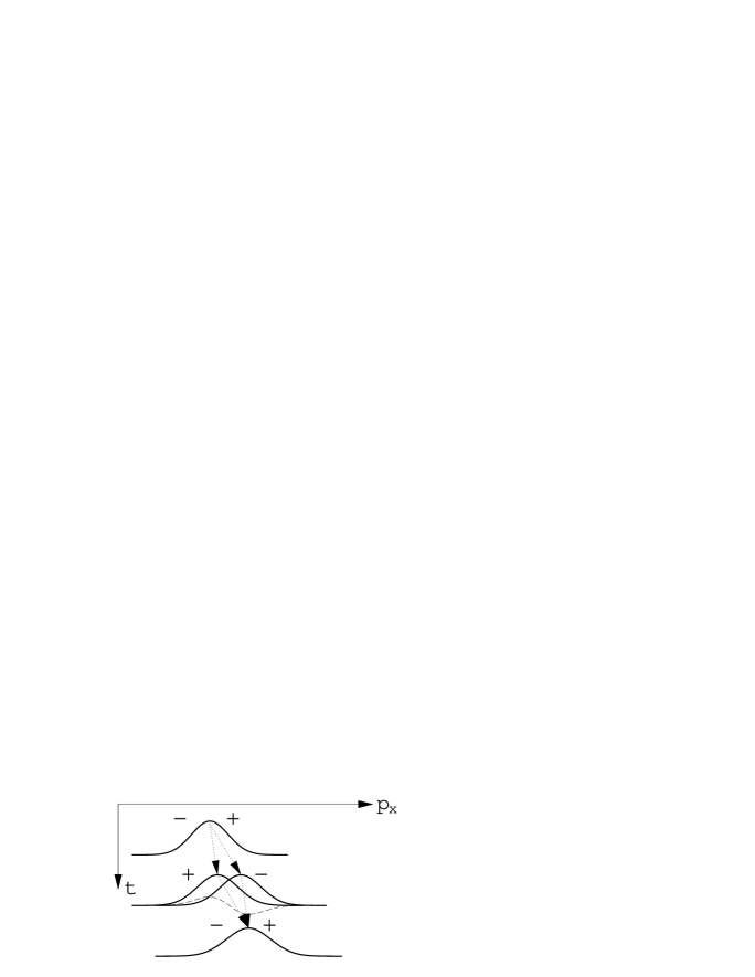
FIG. 8.: Illustration of ‘recoil-induced magnetization’ in a $TE$ polarized evanescent wave. The momentum distributions for the sublevels $|\pm 1/2\rangle_{y}$ (denoted by ‘$+$’ and ‘$-$’) are shifted by the radiation pressure forces ${\bf F}_{\pm}$. Due to the difference in recoil momentum per pumping cycle, the sublevel distributions separate and merge periodically at the optical pumping rate. The dashed line shows the net magnetization $J_{y}(p_{x})$ as a function of the momentum component $p_{x}$ parallel to the evanescent wave’s propagation vector.

c Experimental signature.

As a consequence of the difference between the radiation pressure forces ${\bf F}_{\mp\rightarrow\pm}(z)$, the atomic Zeeman sublevels absorb different momenta per optical pumping time. Their distributions hence separate in momentum space. But since the sublevels have been exchanged in the pumping cycle, the sublevel momentum distributions $w_{\pm}(p_{x})$ merge again after a second pumping cycle. The process is then repeated periodically in time, as shown schematically in Fig. 8. The maximum sublevel separation in momentum space is of the order of a few photon momenta

$$\max\delta{\bf p}\simeq\frac{{\bf F}_{+\rightarrow-}^{\prime}-{\bf F}_{-\rightarrow+}}{\Gamma^{\prime}_{\sigma}}=-4\hbar k{\bf e}_{x}\frac{a_{1}(z;0)}{c_{\|}(z)+c_{\perp}(z)}$$ (162)

We note that in the transient regime, this phenomenon may be observed experimentally using similar techniques as for atomic diffraction experiments at normal incidence [58]. For longer interaction times, one could think of Raman spectroscopy to detect the Zeeman sublevel imbalance as a function of the velocity $p_{x}/M$: Eq.(154) indeed predicts a magnetization $w_{+}-w_{-}\equiv J_{y}$ proportional to the derivative $\partial w/\partial p_{x}$ of the atomic momentum distribution (‘recoil-induced magnetization’). Note that the periodic separation of the sublevels might be difficult to observe because their momentum distributions are also broadened by spontaneous emission (momentum diffusion).

IV Conclusion

We have formulated a theoretical framework to describe the motion of an atom that is fluorescing in an environment with modified electromagnetic field modes. We provided expressions for the radiation pressure force and the momentum diffusion tensor in the limits of low, but semiclassical velocites and low saturation. This general theory applies to atoms with arbitrary Zeeman sublevel structure and environments with arbitrary electromagnetic field correlations. One important result is that the internal and external (center-of-mass) dynamics of the atoms is determined by the two-point correlation tensor of the vacuum field around the atomic position. We then made explicit predictions for simple atoms ($J_{g}=0,\,1/2$) in the vicinity of a flat dielectric surface. These results allow for precise estimates of the effects of spontaneous emission when atoms are either reflected from an evanescent wave mirror [15, 16, 18] or trapped in a two-dimensional waveguide-like field configuration in the vicinity of a surface [19, 20, 21, 22, 23, 24, 25].

Even for a scalar atom ($J_{g}=0$ ground state), the radiation pressure force exhibits quantitative and qualitative changes with respect to free space. It is increased both due to the subwavelength structure of the evanescent driving field and the modified vacuum correlations. In particular, the radiation pressure is no longer parallel to the phase gradient of the driving field due to the partial reflection at the dielectric interface. The optical pumping of a $J_{g}=1/2$ atom in an evanescent wave shows similar modifications. The atomic magnetization vector is related to the field’s helicity in an anisotropic manner, and even a linearly polarized field gives rise to an imbalance of the atomic sublevel populations in velocity space (‘recoil-induced magnetization’). The sublevel-selective detection of atoms reflected from an evanescent wave mirror is thus a sensitive probe of the electromagnetic field in the simple half-cavity realized by the vacuum–dielectric interface.

The present work might be pursued in two directions: first, one could further explore the properties of radiation pressure in evanescent waves and consider situations beyond the simple models studied in this paper. Let us mention some topics of particular interest: angular momenta $J_{g}\geq 1$ because such atoms are actually used in experiments; the coupling between Zeeman sublevel populations and coherences for more complex field polarizations ($TM$, circular); and the momentum diffusion for Zeeman-degenerate atoms [59]. One may also expect that the combination of relaxation processes and the center-of-mass motion in different light-shift potentials leads to a variety of motion-induced magnetizations, similar to the case of conservative couplings explored in reflection beam-splitters [55] and diffraction gratings [56, 57]. A second direction opens up if one considers different geometries: cold atoms trapped in high-quality cavities, e.g., are currently receiving much interest in the fields of cavity QED and nonlinear quantum optics. The generalized optical Bloch equations derived in Sec. II could be used in their present form to study atomic motion in semiclassical driving fields and might be generalized to describe more complex phenomena as, e.g., the absorption and transmission of a probe field or the influence of the atoms on the cavity properties.

A Derivation of the G.O.B.E. (16)

We outline here the derivation of the quantum-mechanical master equation (16). The only difference to the usual treatments [29] is the quantization of the atomic center-of-mass motion, i.e., we take care of the ordering of the atomic position and momentum operators ${\bf R},{\bf P}$. We only present the case without an external driving field, since this field may be easily accounted for by adding a commutator with the interaction Hamiltonian $V_{AL}$ (3) to the master equation of the reduced density matrix. We also assume that the electromagnetic field is at zero temperature (in the vacuum state), as is usual for optical frequencies.

In the interaction representation (with respect to the free atomic Hamiltonian $H_{0}$ plus the free vacuum field Hamiltonian $H_{R}$), the evolution of the full atom + reservoir density matrix $\rho_{AR}$ is given by

$$\dot{\rho}_{AR}=\frac{1}{i\hbar}\left[{V}_{AR}(t),\rho_{AR}\right]$$ (A1)

with the atom-field interaction given by the electric dipole interaction

$$V_{AR}(t)=-{\cal D}{\bf d}(t)\cdot{\bf E}({\bf R},t)$$ (A2)

Here, ${\bf D}(t)={\cal D}{\bf d}(t)$ is the atomic dipole operator and ${\bf E}({\bf r},t)$ the electric field operator in the Heisenberg picture (these operators evolve in time according to the Hamiltonian $H_{0}+H_{R}$). Anticipating the approximation of slowly moving atoms, we neglect in Eq.(A2) the time-dependence of the position operator ${\bf R}$ due to $H_{0}$ (free flight).

To solve Eq.(A1) in second-order perturbation theory, we first re-write it as an integral equation:

$$\rho_{AR}(t+\Delta t)=\rho_{AR}(t)+\frac{1}{i\hbar}\int\limits_{t}^{t+\Delta t}\!d\tau\,\left[{V}_{AR}(\tau),\rho_{AR}(\tau)\right]$$ (A3)

This equation is iterated by inserting a similar expression for $\rho_{AR}(\tau)$ under the integral sign. Taking then the trace over the vacuum field variables, one obtains the master equation for the reduced atomic density matrix $\rho$. As usual in perturbation theory, the second-order term in ${V}_{AR}$ is simplified by factorizing the full density matrix according to $\rho_{AR}(\tau)=\rho(\tau)\otimes\rho_{\text{vac}}$. The resulting master equation reads in the position representation

$$\langle{\bf r}_{1}|\rho(t+\Delta t)|{\bf r}_{2}\rangle=\langle{\bf r}_{1}|\rho(t)|{\bf r}_{2}\rangle+\frac{{\cal D}^{2}}{\hbar^{2}}\int\limits_{t}^{t+\Delta t}\!d\tau^{\prime}\int\limits_{t}^{\tau^{\prime}}\!d\tau\sum\limits_{i,j=x,y,z}$$ (A4)

$$\Big{\{}-\,\langle E_{i}^{(+)}({\bf r}_{1},\tau^{\prime})E_{j}^{(-)}({\bf r}_{1},\tau)\rangle\,d_{i}(\tau^{\prime})d_{j}(\tau)\langle{\bf r}_{1}|\rho(\tau)|{\bf r}_{2}\rangle$$ (A5)

$$-\,\langle E_{i}^{(+)}({\bf r}_{2},\tau)E_{j}^{(-)}({\bf r}_{2},\tau^{\prime})\rangle\,\langle{\bf r}_{1}|\rho(\tau)|{\bf r}_{2}\rangle d_{i}(\tau)d_{j}(\tau^{\prime})$$ (A6)

$$+\,\langle E_{i}^{(+)}({\bf r}_{2},\tau)E_{j}^{(-)}({\bf r}_{1},\tau^{\prime})\rangle\,d_{j}(\tau^{\prime})\langle{\bf r}_{1}|\rho(\tau)|{\bf r}_{2}\rangle d_{i}(\tau)$$ (A7)

$$+\,\langle E_{i}^{(+)}({\bf r}_{2},\tau^{\prime})E_{j}^{(-)}({\bf r}_{1},\tau)\rangle\,d_{j}(\tau)\langle{\bf r}_{1}|\rho(\tau)|{\bf r}_{2}\rangle d_{i}(\tau^{\prime})\Big{\}}.$$ (A8)

For brevity, we did not write out the vacuum state for the field expectation value $\langle 0|E_{i}^{(+)}({\bf r}_{1},\tau^{\prime})E_{j}^{(-)}({\bf r}_{2},\tau)|0\rangle$ where ${\bf E}^{(\pm)}({\bf r},t)$ are the positive and negative frequency components of the field operator.

We now explicit the free evolution of the atomic dipole operator for a two-manifold system

$${\bf d}(\tau)={\bf d}^{-}e^{-i\omega_{A}(\tau-t)}+{\bf d}^{+}e^{i\omega_{A}(\tau-t)},$$ (A9)

where ${\bf d}^{\pm}$ are the dipole raising and lowering operators in the Schrödinger picture at time $t$. We observe that the correlation time of the vacuum field fluctuations is much shorter than the timescale $\Delta t$ for the evolution of the atomic density matrix. This implies that we may compute the time integrals in Eq.(A8) in the usual way [47]: replace $\tau$ by $t$ in the argument of the density matrix and take the latter outside the integral; change to the integration variable $\tau^{\prime}-\tau$ and replace its border $\Delta t$ by infinity; discard terms oscillating at twice the optical frequency; identify the Fourier transform of the two-time vacuum field correlations at the atomic frequency:

$${\cal E}^{i,j}({\bf r}_{1},{\bf r}_{2})=$$ (A10)

$$=\int\limits_{-\infty}^{\infty}\!d(\tau^{\prime}-\tau)\langle E_{i}^{(+)}({\bf r}_{1},\tau^{\prime})E_{j}^{(-)}({\bf r}_{2},\tau)\rangle e^{i\omega_{A}(\tau^{\prime}-\tau)}$$ (A11)

The remaining time integral then turns out to be proportional to $\Delta t$, and after some term rearrangements, one obtains the following form for the master equation (summation over repeated indices is understood)

$$\langle{\bf r}_{1}|\frac{\rho(t+\Delta t)-\rho(t)}{\Delta t}|{\bf r}_{2}\rangle=$$ (A12)

$$=-\,\frac{{\cal D}^{2}}{2\hbar^{2}}\langle{\bf r}_{1}|\Big{\{}{\cal E}^{i,j}({\bf R},{\bf R})d_{i}^{+}d_{j}^{-},\,\rho(t)\Big{\}}|{\bf r}_{2}\rangle$$ (A13)

$$\quad+\,\frac{{\cal D}^{2}}{\hbar^{2}}{\cal E}^{i,j}({\bf r}_{2},{\bf r}_{1})d_{j}^{-}\langle{\bf r}_{1}|\rho(t)|{\bf r}_{2}\rangle d_{i}^{+}$$ (A14)

$$\quad+\,\frac{1}{i\hbar}\langle{\bf r}_{1}|\left[(H_{A}({\bf R})-H_{0}),\,\rho(t)\right]|{\bf r}_{2}\rangle$$ (A15)

We may identify the lhs of this equation with the time derivative $\langle{\bf r}_{1}|\dot{\rho}|{\bf r}_{2}\rangle$ since the reduced density matrix evolves slowly on the time scale of the vacuum fluctuations.

We finally recall that the correlation function (A10) is identical, up to a normalization, to the field correlation tensor defined in Eq.(18): $({\cal D}^{2}/\hbar^{2}){\cal E}^{i,j}=\Gamma_{\infty}C^{i,j}$. The first two lines of Eq.(A12) are then readily identified with the relaxation part $\dot{\rho}_{relax}$ of the G.O.B.E. (16). Furthermore, the last line of Eq.(A12) contains the level shifts (Lamb-shifts) due to the coupling to the reservoir. These shifts contain both the renormalization of the atomic Hamiltonian, $H_{A,\infty}-H_{0}$, and its the interface-dependent part $\Delta H_{A}({\bf R})$ appearing in Eq.(8). For simplicity, we do not write down explicit expressions and refer to Ref.[41] for a discussion of the atomic level shifts in the vicinity of a vacuum–dielectric interface.

B Adiabatic elimination of the optical coherences and the excited state population

In this appendix, we analyze in detail the validity conditions for the adiabatic elimination of the optical coherences and the excited state density matrix.

1 Optical coherences

The atoms are driven by a laser field that we describe by a monochromatic classical field

$${\cal{\vec{E}}}_{L}({\bf r},t)={\cal{\vec{E}}}_{L}({\bf r})e^{-i\omega_{L}t}+\text{c.c.}$$ (B1)

The interaction Hamiltonian (3) becomes, in the rotating wave approximation,

$$V_{AL} = -{\cal D}\left({\bf d}^{+}.{\cal{\vec{E}}}_{L}({\bf r})e^{-i\omega_{L}t}+{\bf d}^{-}.{\cal{\vec{E}}}_{L}^{*}({\bf r})e^{i\omega_{L}t}\right)$$ (B2)

$$= -{\cal D}{\cal E}_{0}\left({\bf d}^{+}.\mathchoice{{\hbox{\boldmath$\displaystyle\xi$}}}{{\hbox{\boldmath$\textstyle\xi$}}}{{\hbox{\boldmath$\scriptstyle\xi$}}}{{\hbox{\boldmath$\scriptscriptstyle\xi$}}}({\bf r})e^{-i\omega_{L}t}+{\bf d}^{-}.\mathchoice{{\hbox{\boldmath$\displaystyle\xi$}}}{{\hbox{\boldmath$\textstyle\xi$}}}{{\hbox{\boldmath$\scriptstyle\xi$}}}{{\hbox{\boldmath$\scriptscriptstyle\xi$}}}^{*}({\bf r})e^{i\omega_{L}t}\right)$$ (B3)

where the dimensionless vector $\mathchoice{{\hbox{\boldmath$\displaystyle\xi$}}}{{\hbox{\boldmath$\textstyle\xi$}}}{{\hbox{\boldmath$\scriptstyle\xi$}}}{{\hbox{\boldmath$\scriptscriptstyle\xi$}}}({\bf r})$ for the field profile [Eq.(23)] has been used. The time-dependence of the interaction Hamiltonian is removed by passing into the “rotating frame”, i.e., we write the optical coherence in the form

$$\rho_{eg}=e^{-i\omega_{L}t}\tilde{\rho}_{eg}$$ (B4)

The equation of motion for $\tilde{\rho}_{eg}$ is now readily obtained from the Bloch equations (6, 7, 8, 16) and reads

$$\bigg{(}\frac{d}{dt}-i\Delta+\frac{\Gamma_{\infty}}{2}{\cal G}_{e}({\bf R})\bigg{)}\tilde{\rho}_{eg}=$$ (B5)

$$=\frac{1}{i\hbar}\bigg{[}P_{e}\Delta H_{A}({\bf R})P_{e}\tilde{\rho}_{eg}-\tilde{\rho}_{eg}P_{g}\Delta H_{A}({\bf R})P_{g}\bigg{]}+$$ (B6)

$$+\frac{1}{i\hbar}\bigg{[}\frac{{\bf P}^{2}}{2M},\,\tilde{\rho}_{eg}\bigg{]}+\frac{i{\cal D}{\cal E}_{0}}{\hbar}\Big{(}[{\bf d}^{+}.\mathchoice{{\hbox{\boldmath$\displaystyle\xi$}}}{{\hbox{\boldmath$\textstyle\xi$}}}{{\hbox{\boldmath$\scriptstyle\xi$}}}{{\hbox{\boldmath$\scriptscriptstyle\xi$}}}({\bf R})]\sigma-\rho_{ee}[{\bf d}^{+}.\mathchoice{{\hbox{\boldmath$\displaystyle\xi$}}}{{\hbox{\boldmath$\textstyle\xi$}}}{{\hbox{\boldmath$\scriptstyle\xi$}}}{{\hbox{\boldmath$\scriptscriptstyle\xi$}}}({\bf R})]\Big{)}$$ (B7)

The ordering of the terms takes into account that ${\bf R}$ is the atomic position operator. We have also introduced the abbreviation

$${\cal G}_{e}({\bf R})\equiv C^{i,j}({\bf R},{\bf R})d^{+}_{i}d^{-}_{j}$$ (B8)

Eq.(B5) may be approximately solved if the detuning $\Delta$ is outweighing all the other frequencies. We therefore assume that the atoms are driven off-resonantly and at low saturation, $|\Delta|\gg\Gamma_{\infty},{\cal D}{\cal E}_{0}/\hbar,|\Delta H_{A}/\hbar|$, as in condition (65). The frequency associated with the kinetic energy operator may be estimated in the Wigner representation [cf. Eq.(49)]. If we assume that the atomic position distribution varies at most on the scale of the optical wavelength, this term is overestimated by the Doppler shift $kp/M$. In this way, we find the third condition appearing in (65), $|\Delta|\gg kp/M$.

Given these conditions, the adiabatic solution to Eq.(B5), correct to first order in $\Gamma_{\infty}/\Delta$, reads

$$\tilde{\rho}_{eg} \simeq -\frac{{\cal D}{\cal E}_{0}}{\hbar\Delta}\Big{(}1-i\frac{\Gamma_{\infty}}{2\Delta}{\cal G}_{e}({\bf R})\Big{)}\times$$ (B10)

$$\times\Big{(}[{\bf d}^{+}.\mathchoice{{\hbox{\boldmath$\displaystyle\xi$}}}{{\hbox{\boldmath$\textstyle\xi$}}}{{\hbox{\boldmath$\scriptstyle\xi$}}}{{\hbox{\boldmath$\scriptscriptstyle\xi$}}}({\bf R})]\sigma-\rho_{ee}[{\bf d}^{+}.\mathchoice{{\hbox{\boldmath$\displaystyle\xi$}}}{{\hbox{\boldmath$\textstyle\xi$}}}{{\hbox{\boldmath$\scriptstyle\xi$}}}{{\hbox{\boldmath$\scriptscriptstyle\xi$}}}({\bf R})]\Big{)}$$

Note that the optical coherence $\tilde{\rho}_{ge}$ is equal to the hermitian conjugate of (B10). We shall see in the next paragraph that the excited state density matrix $\rho_{ee}$ is much smaller than the ground state density matrix $\sigma$ [Eq.(B22)]. We may therefore neglect the former in Eq.(B10). Using the definition (22) of the reduced dipole operator ${\bf b}^{-}({\bf R})$ and recalling that the projection operator $\sum_{i}d^{+}_{i}d^{-}_{i}=P_{e}$ acts as the identity onto the excited state manifold, one sees that Eq.(B10) yields the expression (35) for the optical coherences.

2 Excited state

The generalized optical Bloch equation for the excited state density matrix $\rho_{ee}$ reads

$$\dot{\rho}_{ee}+\frac{\Gamma_{\infty}}{2}\bigg{\{}{\cal G}_{e}({\bf R}),\,\rho_{ee}\bigg{\}}=$$ (B11)

$$=\frac{1}{i\hbar}\bigg{[}\frac{{\bf P}^{2}}{2M}+P_{e}\Delta H_{A}({\bf R})P_{e},\,\rho_{ee}\bigg{]}+$$ (B12)

$$+\frac{i{\cal D}{\cal E}_{0}}{\hbar}\Big{(}[{\bf d}^{+}.\mathchoice{{\hbox{\boldmath$\displaystyle\xi$}}}{{\hbox{\boldmath$\textstyle\xi$}}}{{\hbox{\boldmath$\scriptstyle\xi$}}}{{\hbox{\boldmath$\scriptscriptstyle\xi$}}}({\bf R})]\tilde{\rho}_{ge}-\tilde{\rho}_{eg}[{\bf d}^{-}.\mathchoice{{\hbox{\boldmath$\displaystyle\xi$}}}{{\hbox{\boldmath$\textstyle\xi$}}}{{\hbox{\boldmath$\scriptstyle\xi$}}}{{\hbox{\boldmath$\scriptscriptstyle\xi$}}}^{*}({\bf R})]\Big{)}$$ (B13)

Inserting the adiabatic solution (B10) for the optical coherences, one obtains

$$\dot{\rho}_{ee}+\frac{\Gamma_{\infty}}{2}\bigg{\{}{\cal G}_{e}({\bf R}),\,\rho_{ee}\bigg{\}}=\frac{1}{i\hbar}\bigg{[}\frac{{\bf P}^{2}}{2M},\,\rho_{ee}\bigg{]}+$$ (B14)

$$\quad+\frac{1}{i\hbar}\bigg{[}P_{e}\Delta H_{A}({\bf R})P_{e}-\hbar\Delta\frac{s_{0}}{2}[{\bf d}^{+}.\mathchoice{{\hbox{\boldmath$\displaystyle\xi$}}}{{\hbox{\boldmath$\textstyle\xi$}}}{{\hbox{\boldmath$\scriptstyle\xi$}}}{{\hbox{\boldmath$\scriptscriptstyle\xi$}}}({\bf R})][{\bf d}^{-}.\mathchoice{{\hbox{\boldmath$\displaystyle\xi$}}}{{\hbox{\boldmath$\textstyle\xi$}}}{{\hbox{\boldmath$\scriptstyle\xi$}}}{{\hbox{\boldmath$\scriptscriptstyle\xi$}}}^{*}({\bf R})],\,\rho_{ee}\bigg{]}$$ (B15)

$$\quad+\frac{\Gamma_{\infty}}{2}\frac{s_{0}}{2}\bigg{\{}{\cal G}_{e}({\bf R}),\,[{\bf d}^{+}.\mathchoice{{\hbox{\boldmath$\displaystyle\xi$}}}{{\hbox{\boldmath$\textstyle\xi$}}}{{\hbox{\boldmath$\scriptstyle\xi$}}}{{\hbox{\boldmath$\scriptscriptstyle\xi$}}}({\bf R})]\sigma[{\bf d}^{-}.\mathchoice{{\hbox{\boldmath$\displaystyle\xi$}}}{{\hbox{\boldmath$\textstyle\xi$}}}{{\hbox{\boldmath$\scriptstyle\xi$}}}{{\hbox{\boldmath$\scriptscriptstyle\xi$}}}^{*}({\bf R})]\bigg{\}}$$ (B16)

$$\quad-\frac{\Gamma_{\infty}}{2}\frac{s_{0}}{2}\Big{(}[{\bf d}^{+}.\mathchoice{{\hbox{\boldmath$\displaystyle\xi$}}}{{\hbox{\boldmath$\textstyle\xi$}}}{{\hbox{\boldmath$\scriptstyle\xi$}}}{{\hbox{\boldmath$\scriptscriptstyle\xi$}}}({\bf R})][{\bf d}^{-}.\mathchoice{{\hbox{\boldmath$\displaystyle\xi$}}}{{\hbox{\boldmath$\textstyle\xi$}}}{{\hbox{\boldmath$\scriptstyle\xi$}}}{{\hbox{\boldmath$\scriptscriptstyle\xi$}}}^{*}({\bf R})]\rho_{ee}{\cal G}_{e}({\bf R})+$$ (B17)

$$\qquad+{\cal G}_{e}({\bf R})\rho_{ee}[{\bf d}^{+}.\mathchoice{{\hbox{\boldmath$\displaystyle\xi$}}}{{\hbox{\boldmath$\textstyle\xi$}}}{{\hbox{\boldmath$\scriptstyle\xi$}}}{{\hbox{\boldmath$\scriptscriptstyle\xi$}}}({\bf R})][{\bf d}^{-}.\mathchoice{{\hbox{\boldmath$\displaystyle\xi$}}}{{\hbox{\boldmath$\textstyle\xi$}}}{{\hbox{\boldmath$\scriptstyle\xi$}}}{{\hbox{\boldmath$\scriptscriptstyle\xi$}}}^{*}({\bf R})]\Big{)}$$ (B18)

We have used the saturation parameter $s_{0}$ defined in Eq.(25).

To solve this equation approximately, we observe that the last term on the rhs is small compared to the term involving $\Gamma_{\infty}$ on the lhs, because of the low saturation limit $s_{0}\ll 1$ [condition (65)]. We also want to neglect the first two lines on the rhs (the kinetic and potential energy operators in the commutator). We noted above that the kinetic energy corresponds to a rate smaller than roughly the Doppler shift. It is hence negligible if condition (63), $\Gamma_{\infty}\gg kp/M$, holds. We note that this condition may be re-written as

$$\frac{1}{\Gamma_{\infty}}\frac{p}{M}\ll\lambdabar$$ (B19)

i.e., the atoms move much less than a wavelength during the lifetime of the excited state. To estimate the potential energy term, we again use the Wigner representation and find [cf. Eq.(49)] that it is of the order of the force $F_{e}$ acting on the excited state divided by the width $\Delta p$ of the atomic momentum distribution. We therefore need to suppose $\Gamma_{\infty}\gg F_{e}/\Delta p$ [cf. Eq.(63)] or

$$\frac{F_{e}}{\Gamma_{\infty}}\ll\Delta p$$ (B20)

The momentum the atoms gain during the excited state’s lifetime is hence negligible compared to the width of the momentum distribution.

Given these conditions, we are left with the equation

$$\bigg{\{}{\cal G}_{e}({\bf R}),\,\rho_{ee}-\frac{s_{0}}{2}[{\bf d}^{+}.\mathchoice{{\hbox{\boldmath$\displaystyle\xi$}}}{{\hbox{\boldmath$\textstyle\xi$}}}{{\hbox{\boldmath$\scriptstyle\xi$}}}{{\hbox{\boldmath$\scriptscriptstyle\xi$}}}({\bf R})]\sigma[{\bf d}^{-}.\mathchoice{{\hbox{\boldmath$\displaystyle\xi$}}}{{\hbox{\boldmath$\textstyle\xi$}}}{{\hbox{\boldmath$\scriptstyle\xi$}}}{{\hbox{\boldmath$\scriptscriptstyle\xi$}}}^{*}({\bf R})]\bigg{\}}\simeq 0$$ (B21)

Using the fact that the spontaneous emission rates are positive for any polarization of the spontaneous photon, it is easy to prove that the solution to (B21) is given by

$$\rho_{ee}\simeq\frac{s_{0}}{2}[{\bf d}^{+}.\mathchoice{{\hbox{\boldmath$\displaystyle\xi$}}}{{\hbox{\boldmath$\textstyle\xi$}}}{{\hbox{\boldmath$\scriptstyle\xi$}}}{{\hbox{\boldmath$\scriptscriptstyle\xi$}}}({\bf R})]\sigma[{\bf d}^{-}.\mathchoice{{\hbox{\boldmath$\displaystyle\xi$}}}{{\hbox{\boldmath$\textstyle\xi$}}}{{\hbox{\boldmath$\scriptstyle\xi$}}}{{\hbox{\boldmath$\scriptscriptstyle\xi$}}}^{*}({\bf R})]$$ (B22)

This expression shows that the excited state density matrix is much smaller than that of the ground state, by a factor of the order of the saturation parameter $s_{0}$. In the position representation, Eq.(B22) yields the result (36).

3 Ground state

The Bloch equation for the ground state density matrix $\sigma$ reads in the position representation

$$\langle{\bf r}_{1}|\dot{\sigma}|{\bf r}_{2}\rangle=\frac{1}{i\hbar}\langle{\bf r}_{1}|\bigg{[}\frac{{\bf P}^{2}}{2M}+P_{g}\Delta H_{A}({\bf R})P_{g},\,\sigma\bigg{]}|{\bf r}_{2}\rangle$$ (B23)

$$+\frac{i{\cal D}{\cal E}_{0}}{\hbar}\Big{(}[{\bf d}^{-}.\mathchoice{{\hbox{\boldmath$\displaystyle\xi$}}}{{\hbox{\boldmath$\textstyle\xi$}}}{{\hbox{\boldmath$\scriptstyle\xi$}}}{{\hbox{\boldmath$\scriptscriptstyle\xi$}}}^{*}({\bf r}_{1})]\langle{\bf r}_{1}|\tilde{\rho}_{eg}|{\bf r}_{2}\rangle-\langle{\bf r}_{1}|\tilde{\rho}_{ge}|{\bf r}_{2}\rangle[{\bf d}^{+}.\mathchoice{{\hbox{\boldmath$\displaystyle\xi$}}}{{\hbox{\boldmath$\textstyle\xi$}}}{{\hbox{\boldmath$\scriptstyle\xi$}}}{{\hbox{\boldmath$\scriptscriptstyle\xi$}}}({\bf r}_{2})]\Big{)}$$ (B24)

$$+\Gamma_{\infty}C^{i,j}({\bf r}_{2},{\bf r}_{1})d^{-}_{j}\langle{\bf r}_{1}|\rho_{ee}|{\bf r}_{2}\rangle$$ (B25)

We now insert the adiabatic expressions (B10, B22) for the optical coherences $\tilde{\rho}_{eg}$ and the excited state density matrix $\rho_{ee}$. The last line of Eq.(B25) readily yields the last line of the optical pumping equation (28). In the second line, involving the optical coherences, we neglect terms of order $s_{0}^{2}$ and obtain the following two contributions

$$\frac{1}{i\hbar}\langle{\bf r}_{1}|\Big{[}H_{ls}({\bf R}),\,\sigma\Big{]}|{\bf r}_{2}\rangle-\frac{\Gamma_{\infty}^{\prime}}{2}\langle{\bf r}_{1}|\Big{\{}{\cal G}({\bf R}),\,\sigma\Big{\}}|{\bf r}_{2}\rangle$$ (B26)

The commutator is due to the real part of the optical coherences (B10) (in phase with the driving field) and is characterized by the light-shift Hamiltonian

$$H_{ls}({\bf R}) = \hbar\Delta\frac{s_{0}}{2}[{\bf d}^{-}.\mathchoice{{\hbox{\boldmath$\displaystyle\xi$}}}{{\hbox{\boldmath$\textstyle\xi$}}}{{\hbox{\boldmath$\scriptstyle\xi$}}}{{\hbox{\boldmath$\scriptscriptstyle\xi$}}}^{*}({\bf R})][{\bf d}^{+}.\mathchoice{{\hbox{\boldmath$\displaystyle\xi$}}}{{\hbox{\boldmath$\textstyle\xi$}}}{{\hbox{\boldmath$\scriptstyle\xi$}}}{{\hbox{\boldmath$\scriptscriptstyle\xi$}}}({\bf R})]$$ (B27)

$$= \hbar\Delta^{\prime}[{\bf d}^{-}.\mathchoice{{\hbox{\boldmath$\displaystyle\xi$}}}{{\hbox{\boldmath$\textstyle\xi$}}}{{\hbox{\boldmath$\scriptstyle\xi$}}}{{\hbox{\boldmath$\scriptscriptstyle\xi$}}}^{*}({\bf R})][{\bf d}^{+}.\mathchoice{{\hbox{\boldmath$\displaystyle\xi$}}}{{\hbox{\boldmath$\textstyle\xi$}}}{{\hbox{\boldmath$\scriptstyle\xi$}}}{{\hbox{\boldmath$\scriptscriptstyle\xi$}}}({\bf R})].$$ (B28)

This Hamiltonian adds to the level shift $P_{g}\Delta H_{A}({\bf R})P_{g}$ in Eq.(B25) to give the effective ground-state Hamiltonian $H_{eff}({\bf R})$ (30). The anticommutator in Eq.(B26) is due to the imaginary part of the optical coherences $\tilde{\rho}_{eg}$ (phase lag of order $\Gamma_{\infty}/\Delta$). It involves the ground-state operator ${\cal G}({\bf R})$ defined in Eq.(32):

$$\frac{\Gamma^{\prime}_{\infty}}{2}{\cal G}({\bf R}) = \frac{\Gamma^{\prime}_{\infty}}{2}C^{i,j}({\bf R},{\bf R})b^{-}_{i}({\bf R})b^{-}_{j}({\bf R})$$ (B29)

$$= \frac{\Gamma_{\infty}}{2}\frac{s_{0}}{2}[{\bf d}^{-}.\mathchoice{{\hbox{\boldmath$\displaystyle\xi$}}}{{\hbox{\boldmath$\textstyle\xi$}}}{{\hbox{\boldmath$\scriptstyle\xi$}}}{{\hbox{\boldmath$\scriptscriptstyle\xi$}}}^{*}({\bf R})]{\cal G}_{e}({\bf R})[{\bf d}^{+}.\mathchoice{{\hbox{\boldmath$\displaystyle\xi$}}}{{\hbox{\boldmath$\textstyle\xi$}}}{{\hbox{\boldmath$\scriptstyle\xi$}}}{{\hbox{\boldmath$\scriptscriptstyle\xi$}}}({\bf R})]$$ (B30)

We have thus obtained the optical pumping equation (28).

C Field correlations for the vacuum–dielectric interface

In this appendix, we outline the calculation of the electromagnetic field correlation tensor for the vacuum–dielectric interface, following Carnaglia and Mandel [48]. We assume that the dielectric fills the half-space $z<0$ and is characterized by the (real) refractive index $n_{0}$.

1 Field modes

Carnaglia and Mandel distinguish two types of electromagnetic field modes for this geometry:

(a) modes incident from inside the dielectric and being partially or totally reflected at the dielectric–vacuum interface. In the vacuum half-space, these modes are either propagating or evanescent, depending on the internal angle of incidence. The wavevector of the incident wave in the dielectric is denoted ${\bf k}_{0\uparrow}$, and the vacuum wavevector of the transmitted wave ${\bf k}_{\uparrow}$. Obviously, one has $|{\bf k}_{0\uparrow}|=n_{0}(\omega/c)\equiv n_{0}k$ and $|{\bf k}_{\uparrow}|=k$. The wavevectors are decomposed according to ${\bf k}_{\uparrow}=({\bf k}_{\|},k_{z})$ where ${\bf k}_{\|}$ denotes the components parallel to the interface plane (the $xy$-plane) and $k_{z}$ the perpendicular component. The parallel components of ${\bf k}_{0}$ and ${\bf k}$ coincide: ${\bf k}_{0\|}={\bf k}_{\|}$. The perpendicular components are such that in the dielectric, $k_{0z}>0$; in vacuum, $k_{z}$ is chosen such that $k_{z}>0$ for the propagating modes and Im $k_{z}>0$ for the evanescent waves. For later convenience, we introduce the abbreviation $u\equiv|{\bf k}_{\|}|/k$. Modes propagating (evanescent) in vacuum then correspond to $0\leq u\leq 1$ ($1<u<n_{0}$), respectively.

We write ${\bf f}_{\uparrow}({\bf k}_{0\uparrow},\mu;{\bf r})$ ($\mu=TE,\,TM$) for the corresponding mode function that is normalized to unit (incident) amplitude in the dielectric. In the vacuum half-space, these modes have an amplitude equal to the Fresnel transmission coefficient denoted by $t(u,\mu)$. Explicitly, one has ($z>0$):

$${\bf f}_{\uparrow}({\bf k}_{0},\mu;{\bf r}) = {\bf e}_{\uparrow}(u,\varphi,\mu)t(u,\mu)\exp{(i{\bf k}_{\uparrow}\cdot{\bf r})},$$ (C1)

$$\text{with}\quad{\bf k} = k(u\cos\varphi,u\sin\varphi,v),$$ (C3)

$$\quad(0\leq u\leq n_{0}),$$

$$v = \sqrt{1-u^{2}},$$ (C4)

$${\bf e}_{\uparrow}(u,\varphi,TE) = (-\sin\varphi,\cos\varphi,0),$$ (C5)

$${\bf e}_{\uparrow}(u,\varphi,TM) = (v\cos\varphi,v\sin\varphi,-u),$$ (C6)

$$t(u,TE) = \frac{2\sqrt{n_{0}^{2}-u^{2}}}{v+\sqrt{n_{0}^{2}-u^{2}}},$$ (C7)

$$t(u,TM) = \frac{2n_{0}^{2}\sqrt{n_{0}^{2}-u^{2}}}{n_{0}^{2}v+\sqrt{n_{0}^{2}-u^{2}}}.$$ (C8)

Note that the $TM$ polarization vector (C6) is complex for evanescent modes ($u>1$).

(b) modes propagating downwards from the upper half-space into the dielectric with wavevectors ${\bf k}_{\downarrow}=({\bf k}_{\|},-k_{z})$ in vacuum and ${\bf k}_{0\downarrow}=({\bf k}_{\|},-k_{0z})$ in the dielectric. In the vacuum half-space, these modes contain a part reflected from the interface with wavevector ${\bf k}^{(r)}_{\downarrow}={\bf k}_{\uparrow}$. We note ${\bf f}_{\downarrow}({\bf k}_{\downarrow},\mu;{\bf r})$ the corresponding mode function (normalized to unit incident amplitude in vacuum) and $r(u,\mu)$ the Fresnel amplitude reflection coefficient ($z>0$):

$${\bf f}_{\downarrow}({\bf k},\mu;{\bf r}) = \exp{(i{\bf k}_{\|}\cdot{\bf r}_{\|})}({\bf e}_{\downarrow}(u,\varphi,\mu)\,e^{-ik_{z}z}+$$ (C10)

$$+{\bf e}^{(r)}_{\downarrow}(u,\varphi,\mu)\,r(u,\mu)e^{ik_{z}z}),$$

$$\text{with}\quad{\bf k}_{\downarrow} = k\left(u\cos\varphi,u\sin\varphi,-v\right),$$ (C12)

$$\quad(0\leq u\leq 1),$$

$${\bf e}_{\downarrow}(u,\varphi,TE) = (-\sin\varphi,\cos\varphi,0)$$ (C13)

$$= {\bf e}^{(r)}_{\downarrow}(u,\varphi,TE)={\bf e}_{\uparrow}(u,\varphi,TE)$$ (C14)

$${\bf e}_{\downarrow}(u,\varphi,TM) = (v\cos\varphi,v\sin\varphi,u)$$ (C15)

$${\bf e}^{(r)}_{\downarrow}(u,\varphi,TM) = (-v\cos\varphi,-v\sin\varphi,u)$$ (C16)

$$= -{\bf e}_{\uparrow}(u,\varphi,TM)$$ (C17)

$$r(u,TE) = \frac{v-\sqrt{n_{0}^{2}-u^{2}}}{v+\sqrt{n_{0}^{2}-u^{2}}}$$ (C18)

$$r(u,TM) = \frac{n_{0}^{2}v-\sqrt{n_{0}^{2}-u^{2}}}{n_{0}^{2}v+\sqrt{n_{0}^{2}-u^{2}}}$$ (C19)

For a detailed discussion of the orthonormalization of these field modes, cf. Ref. [48].

2 Vacuum field correlation function

Upon quantization, the electric field operator in the vacuum half-space may be written as a sum over the two types of modes introduced above, the mode functions being multiplied by the usual creation and annihilation operators [48, 60]. Using the bosonic commutation rules, Carnaglia and Mandel obtain the following result for the vacuum correlation tensor ($z_{1},z_{2}>0$):

$$\langle 0|E_{i}^{(+)}({\bf r}_{1},\tau)\,E_{j}^{(-)}({\bf r}_{2},0)|0\rangle=$$ (C20)

$$=\int_{>}\!\frac{d^{3}k_{0\uparrow}}{(2\pi)^{3}}\frac{\hbar\omega}{2n_{0}^{2}\varepsilon_{0}}\sum_{\mu}f_{\uparrow i}({\bf k}_{0\uparrow},\mu;{\bf r}_{1})f_{\uparrow j}^{*}({\bf k}_{0\uparrow},\mu;{\bf r}_{2})\,e^{-i\omega\tau}$$ (C21)

$$+\,\int_{<}\!\frac{d^{3}k_{\downarrow}}{(2\pi)^{3}}\frac{\hbar\omega}{2\varepsilon_{0}}\sum_{\mu}f_{\downarrow i}({\bf k}_{\downarrow},\mu;{\bf r}_{1})f_{\downarrow j}^{*}({\bf k}_{\downarrow},\mu;{\bf r}_{2})\,e^{-i\omega\tau}$$ (C22)

The signs “$>$, $<$” on the integral signs are to remind that the wavevectors ${\bf k}_{0\uparrow}$ and ${\bf k}_{\downarrow}$ only run through a half-space.

From expression (C20), we may readily read off the Fourier transform ${\cal E}^{i,j}({\bf r}_{1},{\bf r}_{2})$ of the correlation tensor defined in Eq.(A10), by using as integration variables the frequency $\omega$ and the polar coordinates $u,\varphi$ of the in-plane vector ${\bf k}_{\|}/k$. After some algebra, one obtains the following representation of the normalized correlation tensor (18):

$$C^{i,j}({\bf r}_{1},{\bf r}_{2})=$$ (C23)

$$=\frac{3}{8\pi}\int\limits_{0}^{n_{0}}\!\frac{du\,u}{\sqrt{n_{0}^{2}-u^{2}}}\int\limits_{0}^{2\pi}\!d\varphi\sum_{\mu}f_{\uparrow i}({\bf k}_{0\uparrow},\mu;{\bf r}_{1})f_{\uparrow j}^{*}({\bf k}_{0\uparrow},\mu;{\bf r}_{2})\,+$$ (C24)

$$+\,\frac{3}{8\pi}\int\limits_{0}^{1}\!\frac{du\,u}{\sqrt{1-u^{2}}}\int\limits_{0}^{2\pi}\!d\varphi\sum_{\mu}f_{\downarrow i}({\bf k}_{\downarrow},\mu;{\bf r}_{1})f_{\downarrow j}^{*}({\bf k}_{\downarrow},\mu;{\bf r}_{2})$$ (C25)

[From here on, the wavevectors ${\bf k}_{\uparrow,\downarrow}$ have magnitude $|{\bf k}_{\uparrow,\downarrow}|=\omega_{0}/c=k$ where $\omega_{0}$ is the atomic transition frequency.] In the following, we show that the correlation function (C23) may be written as a sum of two parts, $C=C_{\infty}+C_{int}$, one corresponding to the free-space correlation function, and the other one representing the influence of the interface.

a Free-space part

The free-space correlation function is obtained from those upward propagating modes that are homogeneous plane waves above the dielectric, on the one hand, and from either the incident or the reflected parts of the downward propagating modes, on the other. These contributions may be combined using the following property of the Fresnel coefficients

$$u<1:\qquad\sqrt{\frac{1-u^{2}}{n_{0}^{2}-u^{2}}}t^{2}(u,\mu)+r^{2}(u,\mu)=1$$ (C26)

that follows from the relation $r=-r^{\prime}$ where $r^{\prime}$ is the reflection coefficient for upward propagating modes (reciprocity), and energy conservation. One finally gets the result

$$C^{i,j}_{\infty}({\bf r}_{1},{\bf r}_{2}) = \frac{3}{8\pi}\int\limits_{0}^{1}\!du\int\limits_{0}^{2\pi}\!d\varphi\frac{u}{\sqrt{1-u^{2}}}\sum_{\mu}$$ (C30)

$$\Big{(}e_{\uparrow i}(u,\varphi,\mu)e^{*}_{\uparrow j}(u,\varphi,\mu)e^{ik_{z}(z_{1}-z_{2})}\,+$$

$$\quad+\,e_{\downarrow i}(u,\varphi,\mu)e^{*}_{\downarrow j}(u,\varphi,\mu)e^{-ik_{z}(z_{1}-z_{2})}\Big{)}\times$$

$$\times\exp[i{\bf k}_{\|}\cdot({\bf r}_{\|,1}-{\bf r}_{\|,2})]$$

If the integral is written in terms of the unit vector ${\bf n}={\bf k}/k$, one recovers the familiar expression for the free-space vacuum correlation tensor that appears in Eq.(21).

Due to translational invariance of the vacuum field, the free-space correlation tensor only depends on the difference vector ${\bf s}\equiv{\bf r}_{2}-{\bf r}_{1}$. From rotational invariance, it follows that the tensor may be decomposed into a scalar part, proportional to the unit tensor, and a quadrupolar part with zero trace, proportional to $s^{i}s^{j}-\frac{1}{3}s^{2}\delta^{i,j}$. More explicitly, the correlation tensor may be written for two neighboring points

$$C^{i,j}_{\infty}({\bf s}) = C^{i,j}_{\infty,0}({\bf s})+C^{i,j}_{\infty,2}({\bf s})$$ (C31)

$$\approx \big{(}1-{\textstyle\frac{7}{30}}k^{2}{\bf s}^{2}\big{)}\delta^{i,j}-{\textstyle\frac{1}{10}}k^{2}\big{(}s^{i}s^{j}-{\textstyle\frac{1}{3}}{\bf s}^{2}\delta^{i,j}\big{)}$$ (C32)

We have limited ourselves to second order in $ks$, which is sufficient to compute the radiation pressure force and the momentum diffusion tensor since the latter involve at most a second derivative of the correlation tensor [cf. Eqs.(53, 55, 60)].

b Interface contribution

The interface-dependent part $C^{i,j}_{int}$ of the field correlations is due to two contributions: the evanescent modes ${\bf f}_{\uparrow}({\bf k}_{0\uparrow},\mu;{\bf r})$ (Eq.(C1) with $1<u<n_{0}$), and the crossed term between waves incident from above and reflected at the interface (the two terms of ${\bf f}_{\downarrow}({\bf k}_{\downarrow},\mu;{\bf r})$ in Eq.(C10)). Collecting these contributions, one has

$$C^{i,j}_{int}({\bf r}_{1},{\bf r}_{2})=$$ (C33)

$$=\frac{3}{8\pi}\int\limits_{1}^{n_{0}}\!du\int\limits_{0}^{2\pi}\!d\varphi\frac{u}{\sqrt{n_{0}^{2}-u^{2}}}\sum_{\mu}$$ (C34)

$$\quad e_{\uparrow i}(u,\varphi,\mu)e_{\uparrow j}^{*}(u,\varphi,\mu)|t(u,\mu)|^{2}\times$$ (C35)

$$\quad\times\exp[i{\bf k}_{\|}({\bf r}_{\|,1}-{\bf r}_{\|,2})+ik_{z}(z_{1}+z_{2})]$$ (C36)

$$+\,\frac{3}{8\pi}\int\limits_{0}^{1}\!du\int\limits_{0}^{2\pi}\!d\varphi\frac{u}{\sqrt{1-u^{2}}}\sum_{\mu}$$ (C37)

$$\quad\Big{(}e_{\downarrow i}(u,\varphi,\mu)e_{\downarrow j}^{(r)*}(u,\varphi,\mu)r^{*}(u,\mu)\,e^{-ik_{z}(z_{1}+z_{2})}\,+$$ (C38)

$$\quad+\,e_{\downarrow i}^{(r)}(u,\varphi,\mu)e_{\downarrow j}^{*}(u,\varphi,\mu)r(u,\mu)\,e^{ik_{z}(z_{1}+z_{2})}\Big{)}\times$$ (C39)

$$\times\exp[i{\bf k}_{\|}({\bf r}_{\|,1}-{\bf r}_{\|,2})]$$ (C40)

(Recall that ${\rm Im}\,k_{z}>0$ in the first integral and $k_{z}>0$ in the second.) It is now evident that the interface contribution only depends on the in-plane difference vector ${\bf s}_{\|}={\bf r}_{\|,2}-{\bf r}_{\|,1}$ and the sum of the distances $z_{1}+z_{2}$.

We perform the integration over the azimuthal angle $\varphi$ with the help of the following formula [61] and its derivatives with respect to $ks_{\|}$

$$\int\limits_{0}^{2\pi}\!d\varphi\,e^{-iks_{\|}u\cos\varphi}=2\pi J_{0}(ks_{\|}u)$$ (C41)

where $J_{0}$ is the Bessel function of zeroth order. We also observe the following property of the Fresnel coefficients

$$n_{0}>u>1:\quad\sqrt{\frac{u^{2}-1}{n_{0}^{2}-u^{2}}}|t(u,\mu)|^{2}=2\,\text{Im}\,r(u,\mu)$$ (C42)

that allows to combine the contributions of reflected and evanescent modes in a compact way. Finally, the correlation tensor is decomposed into its isotropic, axial and quadrupolar parts, according to

$$C^{i,j}_{int}(z;{\bf s}_{\|})=C^{i,j}_{int}({\bf r}-{\textstyle\frac{1}{2}}{\bf s},{\bf r}+{\textstyle\frac{1}{2}}{\bf s})$$ (C44)

$$=C^{i,j}_{int,0}(z;{\bf s}_{\|})+C^{i,j}_{int,1}(z;{\bf s}_{\|})+C^{i,j}_{int,2}(z;{\bf s}_{\|})$$ (C45)

$$C^{i,j}_{int,0}(z;{\bf s}_{\|})=c_{0}(z;{\bf s}_{\|}^{2})\delta^{i,j}$$ (C46)

$$C^{i,j}_{int,1}(z;{\bf s}_{\|})=ka(z;{\bf s}_{\|}^{2})\Big{(}\delta^{z,i}s_{\|}^{j}-s_{\|}^{i}\delta^{z,j}\Big{)}$$ (C47)

$$C^{i,j}_{int,2}(z;{\bf s}_{\|})=q_{0}(z;{\bf s}_{\|}^{2})\Big{(}\delta^{i,z}\delta^{j,z}-{\textstyle\frac{1}{3}}\delta^{i,j}\Big{)}+$$ (C48)

$$\quad+k^{2}q_{2}(z;{\bf s}_{\|}^{2})\Big{(}s_{\|}^{i}s_{\|}^{j}-{\textstyle\frac{1}{2}}{\bf s}_{\|}^{2}(\delta^{i,j}-\delta^{i,z}\delta^{j,z})\Big{)}$$ (C49)

In these expressions, the dimensionless weight functions $c_{0},q_{0},a,q_{2}$ are given by the Sommerfeld integrals

$$c_{0}(z;{\bf s}_{\|}^{2}) = \frac{1}{2}\,\text{Re}\int_{0}^{n_{0}}\!\frac{du\,u}{v}\,J_{0}(ks_{\|}u)\times$$ (C52)

$$\times(r_{TE}+(2u^{2}-1)r_{TM})\exp{2ikzv}$$

$$q_{0}(z;{\bf s}_{\|}^{2}) = \frac{3}{4}\,\text{Re}\int_{0}^{n_{0}}\!\frac{du\,u}{v}\,J_{0}(ks_{\|}u)\times$$ (C54)

$$\times(-r_{TE}+(u^{2}+1)r_{TM})\exp{2ikzv}$$

$$a(z;{\bf s}_{\|}^{2}) = \frac{3}{2}\,\text{Im}\int_{0}^{n_{0}}\!du\,u^{2}\,\frac{J_{1}(ks_{\|}u)}{ks_{\|}}r_{TM}\exp{2ikzv}$$ (C55)

$$q_{2}(z;0) = \frac{3}{2}\,\text{Re}\int_{0}^{n_{0}}\!\frac{du\,u}{v}\frac{J_{2}(ks_{\|}u)}{(ks_{\|})^{2}}\times$$ (C57)

$$\times(r_{TE}-(u^{2}-1)r_{TM})\exp{2ikzv}$$

These integrals are computed numerically and are plotted as a function of $kz$ in Fig. 1 for $s_{\|}=0$. The refractive index is $n_{0}=1.5$.

3 Relation to field susceptibility

As a final comment, we would like to display the link between the vacuum correlation tensor on the one hand, and the classical field susceptibility, on the other. The latter quantity gives the (positive-frequency) electric field created at position ${\bf r}_{1}$ by an oscillating dipole located at ${\bf r}_{2}$:

$$E_{i}({\bf r}_{1})e^{-i\omega t}=G^{i,j}({\bf r}_{1},{\bf r}_{2})D_{j}e^{-i\omega t}.$$ (C58)

The tensor $G^{i,j}$ may be calculated from classical electrodynamics [62, 63, 64]. For the vacuum–dielectric interface, we have checked the following relation to the vacuum correlation tensor

$${\cal E}^{i,j}({\bf r}_{1},{\bf r}_{2})=2\hbar\,{\rm Im}\,G^{i,j}({\bf r}_{1},{\bf r}_{2}).$$ (C59)

This result shows that, at least for zero temperature and a two-level system, both the spontaneous emission rates and the associated forces may be calculated from a classical field calculation alone, without explicitly quantizing the field. In particular, Eq.(C59) justifies our interpretation of the radiation pressure force in terms of a classical picture where the atomic dipole interacts with its own radiation reaction field reflected from the vacuum–dielectric interface.

D Optical pumping in a $TM$-polarized evanescent wave

In this appendix, we study the optical pumping of a $J=1/2$ atom in an evanescent wave with $TM$ polarization. The helicity (131) is parallel to the $y$-axis that we choose as the quantization axis. The field is then a superposition of $\sigma^{+}$ and $\sigma^{-}$ circular components, and the light-shift operator (a) is diagonal. It may also be verified from the optical pumping equation Eq.(a) that the magnetization components $J_{x,z}$ decouple from $J_{y}$ and the total population. Assuming that the atoms are initially unpolarized, the pumping process only depends on $J_{y}$ whose evolution is given by (we put again $w=1$ in the optical pumping equation)

$$\left.\frac{\partial J_{y}}{\partial t}\right|_{0} = -\Gamma_{p}(z)-\Gamma_{y,relax}(z)J_{y}$$ (D2)

$$\Gamma_{p}(z) = 2\alpha^{2}\Gamma^{\prime}_{\infty}e^{-2\kappa z}c_{\|}(z)\frac{2\kappa Q}{k^{2}}$$ (D3)

$$\Gamma_{y,relax}(z) = 2\alpha^{2}\Gamma^{\prime}_{\infty}e^{-2\kappa z}c_{\|}(z)\frac{\kappa^{2}+Q^{2}}{k^{2}}$$ (D4)

Optical pumping hence builds up a net magnetization along the negative $y$ axis with a rate $\Gamma_{p}(z)$ that only depends on the fluorescence rate $\Gamma_{\infty}c_{\|}(z)$ for a polarization parallel to the interface. This may be understood from the rate equations for the populations $w_{\pm}=\frac{1}{2}(1\pm J_{y})$ of the Zeeman sublevels $|\pm 1/2\rangle_{y}$ with respect to the $y$ axis. From Eqs.(D), the following rate equations are easily found

$$\frac{\partial w_{+}}{\partial t} = -\Gamma_{+\to-}(z)w_{+}+\Gamma_{-\to+}(z)w_{-}$$ (D6)

$$\frac{\partial w_{-}}{\partial t} = -\Gamma_{-\to+}(z)w_{-}+\Gamma_{+\to-}(z)w_{+}$$ (D7)

$$\Gamma_{-\to+}(z) = {\textstyle\frac{1}{2}}[\Gamma_{y,relax}(z)-\Gamma_{p}(z)]$$ (D8)

$$= 2\alpha^{2}\Gamma_{\infty}^{\prime}\,e^{-2\kappa z}c_{\|}(z)\frac{(\kappa-Q)^{2}}{2k^{2}}$$ (D9)

$$\Gamma_{+\to-}(z) = {\textstyle\frac{1}{2}}[\Gamma_{y,relax}(z)+\Gamma_{p}(z)]$$ (D10)

$$= 2\alpha^{2}\Gamma_{\infty}^{\prime}\,e^{-2\kappa z}c_{\|}(z)\frac{(\kappa+Q)^{2}}{2k^{2}}$$ (D11)

As expected, the rate for the transition $|-1/2\rangle_{y}\to|+1/2\rangle_{y}$, e.g., is proportional to the square $|\xi_{0+}|^{2}=|(\kappa-Q)/\sqrt{2}k|^{2}$ of the amplitude of the $\sigma^{+}$ polarization in the evanescent field (the circular polarization being defined with respect to the $y$ axis). In this process, the atom absorbs a $\sigma_{+}$ polarized photon from the driving field and spontaneously emits a $\pi$ polarized photon (cf. Fig. 7c). The electric field of the latter being parallel to the $y$ axis, the spontaneous transition rate is proportional to the coefficient $C^{y,y}(z)=c_{\|}(z)$ of the vacuum correlation tensor.

The opposite transition $|+1/2\rangle_{y}\to|-1/2\rangle_{y}$ has a larger rate (D11) because in the $TM$ case, the amplitude $\xi_{0-}=(\kappa+Q)/\sqrt{2}k$ of the $\sigma^{-}$ polarization is stronger than $\xi_{0+}$. The steady-state magnetization is not maximum, however, because the pumping rate $\Gamma_{p}$ (D3) is smaller than the relaxation rate $\Gamma_{y,relax}$ (D4), the polarization of the $TM$ evanescent wave being not purely circular. The steady-state solution of the Eq.(D) yields

$$w_{-}^{(stat)}-w_{+}^{(stat)}=-J_{y}^{(stat)}=$$ (D12)

$$=\frac{\Gamma_{p}(z)}{\Gamma_{y,relax}(z)}=\frac{2\kappa Q}{\kappa^{2}+Q^{2}}<1,$$ (D13)

as stated in the text.

REFERENCES

- [1] A. Einstein, Physik. Zeitschr. 18, 121 (1917).
- [2] T. W. Hänsch and A. L. Schawlow, Opt. Commun. 13, 68 (1975).
- [3] R. J. Cook, Phys. Rev. A 22, 1078 (1980).
- [4] J. P. Gordon and A. Ashkin, Phys. Rev. A 21, 1606 (1980).
- [5] J. Dalibard and C. Cohen-Tannoudji, J. Phys. B 18, 1661 (1985).
- [6] C. Adams, M. Siegel, and J. Mlynek, Phys. Rep. 240, 143 (1994).
- [7] T. Pfau et al., Phys. Rev. Lett. 73, 1223 (1994).
- [8] R. J. Cook and R. K. Hill, Opt. Commun. 43, 258 (1982).
- [9] V. I. Balykin, V. S. Letokhov, Y. B. Ovchinnikov, and A. I. Sidorov, Pis’ma Zh. Eksp. Teor. Fiz. 45, 282 (1987) [JETP Lett. 45, 353–356 (1987)].
- [10] M. A. Kasevich, D. S. Weiss, and S. Chu, Opt. Lett. 15, 607 (1990).
- [11] C. G. Aminoff et al., Phys. Rev. Lett. 71, 3083 (1993).
- [12] A. Aspect, C. Henkel, G. Labeyrie, and A. Landragin, in Coherent and Collective Interactions of Particles and Radiation Beams (Proceedings of the International School of Physics “Enrico Fermi”, Course CXXXI, Varenna 1995), edited by A. Aspect, W. Barletta, and R. Bonifacio (IOS Press, Amsterdam, 1996), pp. 551–574.
- [13] W. Seifert et al., Phys. Rev. A 49, 3814 (1994).
- [14] M. Christ et al., Opt. Commun. 107, 211 (1994).
- [15] Y. B. Ovchinnikov, D. V. Laryushin, V. I. Balykin, and V. S. Lethokhov, Pis’ma Zh. Eksp. Teor. Fiz. 62, 102 (1995) [JETP Lett. 62, 113–118 (1995)].
- [16] P. Desbiolles, M. Arndt, P. Szriftgiser, and J. Dalibard, Phys. Rev. A 54, 4292 (1996).
- [17] A. Landragin et al., Phys. Rev. Lett. 77, 1464 (1996).
- [18] W. Power, T. Pfau, and M. Wilkens, Opt. Commun. 143, 125 (1997).
- [19] Y. B. Ovchinnikov, J. Söding, and R. Grimm, Pis’ma Zh. Eksp. Teor. Fiz. 61, 23 (1995) [JETP Lett. 61, 21 (1995)].
- [20] P. Desbiolles and J. Dalibard, Opt. Commun. 132, 540 (1996).
- [21] J. P. Dowling and J. Gea-Banacloche, in Adv. At. Mol. Opt. Phys., edited by P. R. Berman (Academic Press, New York, 1997), Vol. 37, Suppl. 3, pp. 1–94.
- [22] M. Chevrollier et al., Opt. Commun. 136, 22 (1997).
- [23] T. Pfau and J. Mlynek, in Ultracold Atoms and Bose-Einstein-Condensation (Proceedings of the European Quantum Electronics Conference, sept. 1996, Hamburg, Germany), Trends in Optics and Photonics Series, edited by K. Burnett (Optical Society of America, Washington D. C., 1996), Vol. 7, p. 33.
- [24] T. Pfau et al., in Quantum Electronics Conference (Optical Society of America, Washington D. C., 1997), Vol. 17.
- [25] Y. B. Ovchinnikov, I. Manek, and R. Grimm, Phys. Rev. Lett. 79, 2225 (1997).
- [26] S. Haroche, in Fundamental Systems in Quantum Optics (Les Houches, Session LIII), edited by J. Dalibard, J.-M. Raimond, and J. Zinn-Justin (North-Holland, Amsterdam, 1992), pp. 767–940.
- [27] K. H. Drexhage, in Progress in Optics XII, edited by E. Wolf (North-Holland, Amsterdam, 1974), pp. 163–232.
- [28] R. R. Chance, A. Prock, and R. Silbey, in Advances in Chemical Physics XXXVII, edited by I. Prigogine and S. A. Rice (Wiley & Sons, New York, 1978).
- [29] G. S. Agarwal, Phys. Rev. A 12, 1475 (1975).
- [30] R. J. Cook and P. W. Milloni, Phys. Rev. A 35, 5081 (1987).
- [31] E. A. Hinds and V. Sandoghdar, Phys. Rev. A 43, 398 (1991).
- [32] K. Yoshida, Phys. Rev. A 48, 1703 (1993).
- [33] F. Treussart et al., Opt. Lett. 19, 1651 (1994).
- [34] H. Taniguchi and H. Ito, Opt. Lett. 19, 1565 (1994).
- [35] K. Kakazu and Y. S. Kim, Phys. Rev. A 50, 1830 (1994).
- [36] W. Jhe and J. W. Kim, Phys. Rev. A 51, 1150 (1995).
- [37] E. Snoeks, A. Lagendijk, and A. Polman, Phys. Rev. Lett. 74, 2459 (1995).
- [38] V. V. Klimov, M. Ducloy, and V. S. Letokhov, J. Mod. Optics 43, 549 (1996).
- [39] C. Girard, O. J. F. Martin, and A. Dereux, Phys. Rev. Lett. 75, 3098 (1995).
- [40] A. Rahmani, P. C. Chaumet, F. de Fornel, and C. Girard, Phys. Rev. A 56, 3245 (1997).
- [41] J.-Y. Courtois, J.-M. Courty, and J. C. Mertz, Phys. Rev. A 53, 1862 (1996).
- [42] B. Dubetsky and P. R. Berman, Phys. Rev. A 53, 390 (1996).
- [43] G. Roosen and C. Imbert, Opt. Commun. 18, 247 (1976).
- [44] S. M. Tan and D. F. Walls, J. Phys. II France 4, 1897 (1994).
- [45] C. Cohen-Tannoudji, in Frontiers in Laser Spectroscopy (Les Houches XXVII 1975), edited by R. Balian, S. Haroche, and S. Liberman (North Holland, Amsterdam, 1977), Vol. 1, p. 3.
- [46] Y. Castin, Ph.D. thesis, Université de Paris VI, 1992.
- [47] L. Mandel and E. Wolf, Optical coherence and quantum optics (Cambridge University Press, Cambridge, 1995).
- [48] C. K. Carnaglia and L. Mandel, Phys. Rev. D 3, 280 (1971).
- [49] C. Cohen-Tannoudji, J. Dupont-Roc, and G. Grynberg, Photons et atomes — Introduction à l’électrodynamique quantique (InterEditions, Paris, 1987), english translation: Photons and Atoms — Introduction to Quantum Electrodynamics (Wiley, New York 1989).
- [50] Y. Castin, K. Berg-Sørensen, J. Dalibard, and K. Mølmer, Phys. Rev. A 50, 5092 (1994).
- [51] J. Dalibard and C. Cohen-Tannoudji, J. Opt. Soc. Am. B 2, 1707 (1985).
- [52] G. I. Opat, S. J. Wark, and A. Cimmino, Appl. Phys. B 54, 396 (1992).
- [53] C. Henkel et al., Laser Physics 4, 1040 (1994).
- [54] C. Cohen-Tannoudji and J. Dupont-Roc, Phys. Rev. A 5, 968 (1972).
- [55] R. Deutschmann, W. Ertmer, and H. Wallis, Phys. Rev. A 48, 4023 (1993).
- [56] D. Gordon and C. M. Savage, Opt. Commun. 130, 34 (1996).
- [57] C. Henkel, K. Mølmer, R. Kaiser, and C. I. Westbrook, Phys. Rev. A 56, 9 (1997).
- [58] A. Landragin et al., Europhys. Lett. 39, 485 (1997).
- [59] Y. Castin and K. Mølmer, J. Phys. B 23, 4101 (1990).
- [60] R. J. Glauber and M. Lewenstein, Phys. Rev. A 43, 467 (1991).
- [61] Handbook of Mathematical Functions, ninth ed., edited by M. Abramowitz and I. A. Stegun (Dover Publications, Inc., New York, 1972).
- [62] J. D. Jackson, Classical Electrodynamics, 2nd ed. (Wiley & Sons, New York, 1975), Chap. 7.
- [63] A. A. Maradudin and D. L. Mills, Phys. Rev. B 11, 1392 (1975).
- [64] G. S. Agarwal, Phys. Rev. A 11, 230 (1975).