Quantum tomography of mesoscopic superpositions of radiation states

Abstract

We show the feasibility of a tomographic reconstruction of Schrödinger cat states generated according to the scheme proposed by S. Song, C.M. Caves and B. Yurke [Phys. Rev. A 41, 5261 (1990)]. We present a technique that tolerates realistic values for quantum efficiency at photodetectors. The measurement can be achieved by a standard experimental setup.

03.65.Bz, 42.50.-p

Optical homodyne tomography [1] is a powerful tool to measure the density operator of a quantum system, with the possibility of detecting purely quantum features of the radiation field. Such technique was suggested in the past to reconstruct the density matrix of superpositions of classically distinguishable quantum states [2, 3], traditionally known as Schrödinger cats, which represent one of the most celebrated examples of highly non classical states. Some experiments have been performed to detect Schrödinger cat states in atomic systems [4]. For radiation, a scheme to detect cat states has been proposed by Song, Caves and Yurke [5], however with no feasibility study for a real experiment, concerning in particular the main problem of quantum efficiency of detectors, which washes out the fringes visibility.

In this paper we analyze a concrete experimental setup for the scheme given in Ref. [5], and propose to detect the output field by means of homodyne tomography. We will examine the effects of quantum efficiency and present a method to compensate them allowing a good reconstruction of the Wigner function of the Schrödinger cat, and recovering the visibility of the experiment, even with quantum efficiency $\eta_{d}=0.3$ at the readout photodetector, and $\eta_{h}=0.8$ at the homodyne detector. Our proposal to reconstruct the Wigner function allows to appreciate the whole anatomy of the cat rather than just hearing its mew from the oscillations in a single quadrature probability distribution. To our knowledge, this is the first method for detecting the density operator of Schrödinger cat states for free radiation, feasible with current technology.

Let us first briefly review the experimental scheme for generating Schrödinger cat states proposed in Ref. [5] (similar setups were later proposed in Refs. [6, 7]). The main idea consists in feeding two orthogonally polarized modes of radiation, called “signal” and “readout”, both initially in the vacuum state, into a parametric amplifier followed by a half-wave plate. The parametric amplifier generates a correlated state of the two modes and the half wave plate rotates the polarization directions by an angle $\theta$. The global state of the two modes at the output of this setup is given by

$$|\psi\rangle=T(\theta)V(r)|0\rangle|0\rangle=\sum_{j=0}^{\infty}\sum_{m=-j}^{j}B_{j,m}|j-m\rangle|j+m\rangle\;,$$ (1)

where $V(r)=\exp[r(a_{S}a_{R}-a^{\dagger}_{S}a^{\dagger}_{R})]$ describes the action of the parametric amplifier, $T(\theta)=\exp[\theta(a_{S}a^{\dagger}_{R}-a^{\dagger}_{S}a_{R})]$ describes the polarization rotator and the coefficients $B_{j,m}$ are given by

$$B_{j,m}= \frac{(-\tan\theta)^{m}(-\tanh r)^{j}}{\cosh r^{2}}\sqrt{\frac{(j+m)!}{(j-m)!}}$$ (3)

$$\sum_{k={max}(0,-m)}^{j}\frac{(j+k)!}{k!(j-k)!(m+k)!}(-\sin^{2}\theta)^{k}\;.$$

The rotation angle $\theta$ and the gain parameter $r$ are related by the back-action-evading condition [8, 5] as $\sin 2\theta=\tanh r$. The following step of the scheme consists in detecting the number of photons at the readout mode. As a consequence of this measurement, given $n_{r}$ photons detected at the readout, the signal mode is reduced to the state

$$|\psi_{S,n_{r}}\rangle=\frac{1}{P(n_{r})}\sum_{j=0}^{\infty}B_{j+\lfloor\frac{n_{r}+1}{2}\rfloor,j-\lfloor\frac{n_{r}}{2}\rfloor}|2j+\pi(n_{r})\rangle\;,$$ (4)

where $\lfloor x\rfloor$ denotes the integer part of $x$, $\pi(n_{r})$ is the parity of $n_{r}$ and $P(k)$ is the probability of detecting $k$ readout photons with a perfect photodetector, namely

$$P(k)=2^{k}\frac{(2k-1)!!}{(2k)!!}\frac{(\sinh r)^{2k}}{(2\sinh^{2}r+1)^{k+1/2}}\;.$$ (5)

In the scheme of Ref. [5], after detection of the readout mode, the signal mode enters a degenerate parametric amplifier with gain parameter $r_{s}$, described by the evolution operator $S(r_{s})=\exp[\frac{1}{2}r_{s}(a_{S}^{2}-a_{S}^{\dagger 2})]$, which increases the distance of the two components of the superposition in the complex plane without changing the oscillating behavior of the number probability distribution. The final state of the signal is then described by the following quadrature probability distribution (the quadrature operator is defined as $\hat{x}_{\phi}=\frac{1}{2}(a^{\dagger}e^{i\phi}+ae^{-i\phi})$)

$$P(X_{S}(\phi)|n_{r})=$$ (6)

$$\frac{(2{\mbox{Re}}\lambda/\pi)^{1/2}}{(2n_{r}-1)!!\sigma^{n_{r}/2}}e^{-2{\mbox{Re}}\lambda X_{S}^{2}(\phi)}\left|H_{n_{r}}(\sqrt{\lambda}X_{S}(\phi))\right|^{2}\;,$$ (7)

where the eigenvalue $X_{S}(\phi)$ of $\hat{x}_{\phi}$ is the field quadrature component at phase $\phi$, $H_{n}$ denotes the Hermite polynomial, $\lambda=[\cos\phi(e^{-2r_{s}}\cosh 2r\cos\phi+i\sin\phi)]^{-1}$ and $\sigma=1+\tan^{2}\phi\;e^{2r_{s}}/\cosh 2r$.

In this work we propose to detect the Schrödinger cat at the signal mode using optical homodyne tomography [1]. This technique consists in measuring the quadratures of radiation at several phases by means of a homodyne detector. The matrix elements of the density operator of the state are then measured as follows

$$\langle\psi|\hat{\rho}|\psi^{\prime}\rangle_{meas}=\overline{\langle\psi|{\cal K}_{\eta_{h}}(x-\hat{x}_{\phi})|\psi^{\prime}\rangle}\;,$$ (8)

where ${\cal K}_{\eta_{h}}$ represents the kernel function given in Refs. [3, 9] which depends on the value of the quantum efficiency of the homodyne detector $\eta_{h}$, while the overbar denotes the average over the experimental data at different phases. The behavior of the kernel function sets the validity limits of the tomographic reconstruction. These depend on the particular representation chosen to specify the density operator. In this work we always reconstruct the density matrix in the photon number representation: this is possible for any value of the quantum efficiency $\eta_{h}>1/2$ [3, 10]. The $\eta_{h}=1/2$ bound for the overall homodyne quantum efficiency is not a severe limitation in a real experiment, since good homodyne detectors can achieve values of $\eta_{h}$ between 0.85 and 0.94 [11].

Let us now consider the effect of non unit quantum efficiency $\eta_{d}$ at the readout photodetector. According to the Mandel-Kelley-Kleiner formula [12], a detector with non unit quantum efficiency is equivalent to a perfect photodetector preceded by a beam splitter with transmissivity $\eta_{d}$. Then, one can see that when $n_{r}$ photons are detected at the readout, the signal mode is left in the following statistical mixture of Schrödinger cat states

$$\hat{\rho}_{S,n_{r}}=\frac{1}{P_{\eta_{d}}(n_{r})}$$ (9)

$$\times\sum_{k=n_{r}}^{\infty}\left(\begin{array}[]{c}k\\ n_{r}\end{array}\right)\eta_{d}^{n_{r}}(1-\eta_{d})^{k-n_{r}}P(k)|\tilde{\psi}_{S,k}\rangle\langle\tilde{\psi}_{S,k}|\;,$$ (12)

where

$$|\tilde{\psi}_{S,k}\rangle=S(r_{s})|\psi_{S,k}\rangle$$ (13)

is the conditional Schrödinger cat state at the signal mode (4) evolved by the degenerate parametric amplifier, and $P_{\eta_{d}}(k)$ is the probability of detecting $k$ readout photons with quantum efficiency $\eta_{d}$, i.e. the Bernoulli convolution of the probability (5). In Fig. 1 we plot a Monte Carlo tomographic reconstruction of the Wigner function of the statistical mixture (12) corresponding to an experiment with $\eta_{d}=0.3$, $\eta_{h}=0.8$, $r=r_{s}=0.4$ and $n_{r}=2$. As expected, the effect of non unit quantum efficiency is to smooth the oscillations in the complex plane, which are the typical signature of quantum interference (notice that the theoretical Wigner function is practically indistinguishable from the one plotted in Fig. 4). Therefore, the resulting state is more similar to a classical mixture of coherent states rather than a Schrödinger cat. The degradation effects on the cat due to non unit $\eta_{d}$ can be seen also in Fig. 2, where the number probability for the same simulation is plotted: the probability still exhibits a non-monotonic behavior, but the even terms no longer vanish. In Fig. 3 we report a simulation of the quadrature probability distribution at $\phi=0$, which would be seen following the original proposal [5], with the corresponding theoretical curve.

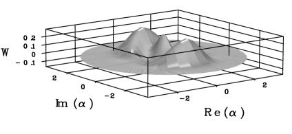
FIG. 1.: Monte Carlo tomographic reconstruction of the Wigner function of the state in Eq. (12), with $\eta_{d}=0.3$, $\eta_{h}=0.8$, $r=r_{s}=0.4$ and $n_{r}=2$. Data are collected for 70 different homodyne phases and $4\cdot 10^{5}$ simulated data are used for each phase.

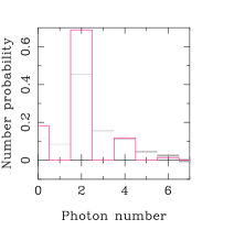
FIG. 2.: Monte Carlo tomographic reconstruction of the probability distribution for the same state and same simulated data of Fig. 1. The simulated values with the corresponding statistical error bars are superimposed to the theoretical values (solid line).

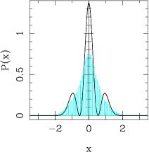
FIG. 3.: Monte Carlo tomographic simulation of the quadrature probability at $\phi=0$ for the same state of Fig. 1. The histogram contains 20000 simulated data, while the solid curve is the theoretical distribution.

We will now present a method to compensate these dramatic effects of realistic quantum efficiencies. The main idea consists in the inversion of formula (12), which gives

$$|\tilde{\psi}_{S,k}\rangle\langle\tilde{\psi}_{S,k}|=P(k)^{-1}\eta_{d}^{-k}$$ (14)

$$\times\sum_{j=0}^{\infty}\left(\begin{array}[]{c}k+j\\ k\end{array}\right)(1-\frac{1}{\eta_{d}})^{j}\hat{\rho}_{S,k+j}P_{\eta_{d}}(k+j)\;.$$ (17)

Hence, a generic $k$-th Schrödinger cat component of the signal mode can be reconstructed by measuring all the signal states corresponding to different readout numbers of photons (larger or equal to $k$), weighting each event according to Eq. (17). In this way we have the additional advantage of using all data with $n_{r}\geq k$ than just those with $n_{r}=k$ of the plain detection in Fig. 1. Moreover, by processing the homodyne data according to Eq. (17) we can reconstruct the whole family of Schrödinger cats $|\tilde{\psi}_{S,k}\rangle$ for different $k$’s at the same time. Notice that this method can be used for the reconstruction of any set of states $|\psi_{S,k}\rangle$ conditioned by an inefficient photodetection.

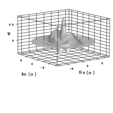
FIG. 4.: Monte Carlo tomographic reconstruction of the Wigner function of the state $|\tilde{\psi}_{S,2}\rangle$ with $\eta_{d}=0.3$, $\eta_{h}=0.8$, $r=r_{s}=0.4$, using the reconstruction algorithm (17). The same number of simulated data as in Fig. 1 is used.

In Fig. 4 we show a tomographic reconstruction of the same Schrödinger cat component of Fig. 1, with the same values of the experimental parameters, but using the reconstruction procedure based on the inversion (17). As we can see, all the oscillations in the Wigner function are properly recovered, and the destructive effects of low quantum efficiencies are defeated. Notice that unlike other compensation methods based on the inverse Bernoulli transformation [13], where the convergence radius of the procedure is $\eta>1/2$, the present method works also for very low values of the quantum efficiency. In our case convergence of the series (17) below the threshold $\eta_{d}=1/2$ is due to the additional decaying factor $P_{\eta_{d}}(k+j)$. An analysis of convergence of the series of errors as in Ref. [10] shows that there is no lower-bound for $\eta_{d}$ if $r\leq\frac{1}{2}\ln(2+\sqrt{3})\simeq 0.658$. Notice that the series convergence is slower for increasing $r$, which corresponds to more excited (macroscopic) Schrödinger cats. This implies that the more macroscopic the cat is, the higher $\eta_{d}$ must be in order to have a good reconstruction.

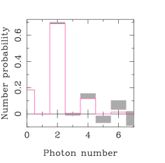
FIG. 5.: Photon number probability of the cat $|\tilde{\psi}_{S,2}\rangle$ using the reconstruction algorithm (17), with the same parameters as in Fig. 4. The simulated values with the corresponding statistical error bars are superimposed to the theoretical values (solid line).

In Fig. 5 we plot the number probability for the same parameters of Fig. 4: the simulated experimental results with corresponding error bars are superimposed to the theoretical value. As we can see, the tomographic reconstruction is very precise and the oscillations of the probability are perfectly resolved. In Fig. 6 we finally report the quadrature probability distribution for $\phi=0$ superimposed to the theoretical curve. The visibility is totally recovered, in contrast to the result in Fig. 3, which would have been obtained according to the original proposal of Ref. [5].

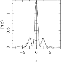
FIG. 6.: Quadrature probability distribution at zero phase of the cat state $|\tilde{\psi}_{S,2}\rangle$, with the same parameters as in Fig. 4. The simulated values with the corresponding statistical error bars are superimposed to the theoretical curve (solid line).

Let us now discuss in more detail the experimental feasibility of the scheme. All the devices needed in the experiment are available with the current technology. The parametric amplification can be realized for example by an ordinary KPT crystal pumped with the second harmonic of a mode locked Nd:Yag pulsed laser working at 80 MHz with 7 ps pulses [14]. The major problem encountered to detect Schrödinger cats in conditional measurement schemes is the cat’s notorious fragility to any kind of losses and inefficiencies. The novelty of the present proposal is that using the reconstruction method based on Eq. (17) low values of $\eta_{d}$ can be tolerated, and hence ordinary linear avalanche photodiodes with $\eta_{d}\sim$0.3 can be used. On the other hand, the tomographic apparatus needed to detect the Schrödinger cat at the signal mode is based on homodyne detection, with the possibility of using high–efficiency photodetectors, because single-photon resolution is no longer needed due to the amplification from the local oscillator (LO). Moreover, the LO comes from the same laser source of the classical pump of the OPA, in order to achieve time matching of modes. In addition, since there is no fluctuating phase in the whole optical setup, neither in the second harmonic generation stage nor in the homodyne detection, the LO is also perfectly phase matched with the pump. The resulting setup is very stable and can take measurements for tens of minutes at a rate of $10^{8}$ data/sec at the readout photodetector. The tomographic reconstructions presented in this paper were obtained with $2.8\cdot 10^{7}$ experimental data. In these examples the probability of detecting less than two photons at the readout photodetector is $\sim 0.9967$. Therefore, taking into account that only the fraction $3.3\cdot 10^{-3}$ of experimental data collected at the readout is useful for the Schrödinger cat reconstruction, we can easily see that the whole set of data can be collected in a few minutes. Notice that increasing $k$, which corresponds to a more excited cat, the number of useful data decreases, and the reconstruction becomes slower. For example, to reconstruct the cat component with $k=4$ only $2\cdot 10^{-5}$ of the experimental data are useful, for $k=5$ we can use only the fraction $1.7\cdot 10^{-6}$ of data, and so on. Moreover, to reconstruct more excited cat components, higher index density matrix elements are needed for the Wigner function, and the effect of statistical errors from tomography becomes more dramatic [15], with the consequence that more data are needed to reach a prescribed accuracy. For these reasons, the more excited the cat is, the longer the experiment and the more difficult the state is to detect. Finally, it has been suggested [16] that by lowering the gain $r$ some (non tomographic) homodyne visibility could be detected for high $\eta_{h}$ ($>0.9$) and for $\eta_{d}$ as low as $0.3$, even without our reconstruction algorithm. However, by lowering the gain the data acquisition rate is greatly reduced, whereas our method works also with high gains.

In conclusion, we have shown the feasibility of a tomographic reconstruction of a Schrödinger cat in an experimental scheme which is practical in a laboratory using standard technology devices. The problem of low efficiencies at the single-photon resolving detector, which was regarded as the major obstacle for experiments of this kind [5], has been solved by the implementation of a suitable tomographic data processing. The whole density matrix of the cat, and hence all its characteristics (such as the photon number probability, the quadrature distribution and the Wigner function), can be measured in this way, whereas the plain homodyne detection proposed in the original scheme of Ref. [5] would not have provided visible probability oscillations with the available low-efficiency single-photon-resolving detectors.

We thank T.F. Arecchi for illuminating discussions on the experimental setup. This work has been supported by the PRA–CAT97 of the INFM.

REFERENCES

- [1] G.M. D’Ariano, Measuring quantum states, in Quantum Optics and the Spectroscopy of Solids, ed. by T. Hakioǧlu and A.S. Shumovsky, Kluwer Academic Publishers (1997), p. 175.
- [2] G.M. D’Ariano, Quant. Semicl. Opt. 7, 693 (1995).
- [3] G. M. D’Ariano, U. Leonhardt and H. Paul, Phys. Rev. A 52, R1801 (1995).
- [4] M. Brune et al., Phys. Rev. Lett. 77, 4887 (1996); J.M. Raimond, M. Brune and S. Haroche, Phys. Rev. Lett. 79, 1964 (1997).
- [5] S. Song, C.M. Caves and B. Yurke, Phys. Rev. A 41, 5261 (1990).
- [6] B. Yurke, W. Schleich and D.F. Walls, Phys. Rev. A 41, R5261 (1990).
- [7] D.-G. Welsch, M. Dakna, L. Knoll and T. Opatrny, e-print quant-ph/9708018.
- [8] A. La Porta, R.E. Slusher and B. Yurke, Phys. Rev. Lett. 62, 28 (1989).
- [9] G.M. D’Ariano, C. Macchiavello and M.G.A. Paris, Phys. Rev. A 50, 4298 (1994).
- [10] G.M. D’Ariano and C. Macchiavello, to appear in Phys. Rev. A (preprint quant-ph/970109).
- [11] G. Breitenbach, S. Schiller and J. Mlynek, Nature 387, 471 (1997).
- [12] L. Mandel, Proc. Phys. Soc. 72,1037 (1958); ibid. 74, 233 (1959); P. L. Kelley and W. H. Kleiner, Phys. Rev. A 30, 844 (1964).
- [13] T. Kiss, U. Herzog, and U. Leonhardt, Phys. Rev. A 52, 2433 (1995).
- [14] T.F. Arecchi, private communication.
- [15] G. M. D’Ariano, C. Macchiavello and N. Sterpi, Quant. Semicl. Opt. 9, 929 (1997).
- [16] A. Montina and T.F. Arecchi, unpublished.