Photon trains and lasing :
The periodically pumped quantum dot

Abstract

We propose to pump semiconductor quantum dots with surface acoustic waves which deliver an alternating periodic sequence of electrons and holes. In combination with a good optical cavity such regular pumping could entail anti-bunching and sub-Poissonian photon statistics. In the bad-cavity limit a train of equally spaced photons would arise.

I Introduction

Semiconductor quantum dots have an interesting potential for quantum optical applications. The growth of dots with transition frequencies in the optical range is very well controlled [1]. Such a zero dimensional system leads to much higher gain than bulk or 2D quantum well structures, as shown theoretically as well as experimentally [1, 2, 3, 4]. Dots as active media in semiconductor lasers have already been established and even lasing of a single dot in a semiconductor microcavity can be achieved [5, 6, 7]. From a theoretical point of view, the discrete states allow to treat dots much like atoms. This makes for a much simpler situation than, for example, the continua of states in quantum wells. Furthermore the semiconductor samples are small compared to atomic beams or even clouds of trapped atoms.
If a dot is to be operated as a low-noise light source it had better be pumped in an as regular manner as possible. Yamamotos scheme of regularizing an injection current by a large resistor [8, 9] could hardly be directed to a single dot. In contrast a surface acoustic (SAW) wave could periodically deliver electrons and holes at a well localized array of dots or even a single dot [10].
The paper is organised as follows. In section II we explain the idea for the pumping mechanism and its theoretical implementation. In section III and IV we give two quantum optical applications of the system, the photon train and the microlaser. We end up with a conclusion and outlook in section V.

II Pump mechanism

To briefly explain our concept, let us consider a semiconductor quantum well surrounded by a piezoelectric material with an interdigital transducer (IDT) on top of the crystal (Fig. 1). A mechanical SAW is generated by applying a HF signal to the IDT. The fundamental acoustic wavelength $\lambda_{0}$ and the frequency $f_{0}=v/\lambda_{0}$ are established by the interdigital electrode spacing, where $v$ is the sound velocity of the crystal. With $\lambda_{0}\sim 1-3\mu m$ and $v\sim 3kms^{-1}$, frequencies in the GHz range are achievable. The acoustic wave is accompanied by a piezoelectric field which gives an additional potential for electrons and holes and so periodically modulates the band edges. For high enough SAW amplitudes, optically generated excitons in the quantum well will be dissociated by the piezoelectric field (inset of Fig. 1). A field strength of the order of $500V/cm$ suffices and results in a wave amplitude of $50-150meV$, depending on the wavelength. Carriers are then trapped in the moving lateral potential superlattice of the sound wave and recombination becomes impossible: Electrons will stay in the minima of the wave, while holes move with the maxima [10]. A simple estimate of the spatial width $\Delta d$ of the lateral ground state in the wave potential yields $\Delta d/\lambda<0.02$. We thus obtain a series of equally spaced quantum wires moving in the plane of the quantum well. The length of these wires is given by the width of the IDTs, typically $300\mu m$. The occupation of the wires with electrons and holes can be controlled by the pump strength of the laser and is of the order $10^{3}-10^{4}$ carriers per wire.
A quantum dot for our purposes may be established by a stressor on top of the crystal which causes a local potential minimum in the quantum well underneeth. The linear dimension of typical stressor dots with transition frequencies in the optical range is about $10-30nm$ while their potential depths are about $100meV$ for electrons and $50meV$ for holes. For further investigations, we assume that there is only one electron and one hole state in the dot. When both states are occupied an exciton is formed, so there is just a single exciton state. We should speak of an exited, a semi-excited, and an unexcited dot when an exciton, only one carrier (electron or hole), and no carrier is present. An excited/unexcited dot may then be treated as simple two-level system with pseudo-spin operators $S^{+},S^{-}$ creating and annihilating an exciton. This system may interact with a single-mode light field. In the semi-excited case no interaction with the light field is possible and the creation of an exciton is only possible by capturing the missing carrier.
While being crossed by a moving quantum wire an empty dot may pluck one of the carriers offered: If the dot potential is deep enough a carrier will drop into it and stay there, while the wave is moving on.
The scheme just sketched may indeed produce the designed properties of the pump. First, the periodicity of arriving carriers is given by the SAW, as the moving wires are well separated. Second, with a density of $\approx 3$ carriers per $100nm$ in a wire, there is a high probability for the dot to capture an electron or hole within the crossing time of a wire. Of course, a single dot makes but inefficient use of the moving wires, as only one of $10^{4}$ carriers is used per cycle. If one had several dots lying in a row parallel to the wires, better pump yields could arise. Another way to increase efficency may be focusing the SAW onto one or few dots, which seems to be feasible in an experiment.
Our periodically pumped dot (PPD) will in practice suffer from degradation of complete regularity. One cause of pump fluctuations is the finite width of the lateral SAW ground state, as mentioned above. This leads to variations in the instant of pumping. Pump noise also results when no carrier is plucked from a crossing wire; this may be minimised by a high electron and hole generation rate in the SAW, so all wires are well occupied. We neglect both types of noise here and consider the case of zero pump fluctuations.
We shall now discuss our pumping scheme in the framework of the Jaynes-Cummings model, limiting ourselves to the single PPD. The system is described by the exciton-field coupling constant $g$, the field damping constant $\kappa$, the pseudo-spin operators $S^{+},S^{-}$ and the photon creation and annihilation operators $a^{{\dagger}},a$. In the interaction picture the master equation for the density operator of dot and cavity mode is

$$\dot{\rho} = g[aS^{+}-a^{{\dagger}}S^{-},\rho]+\frac{\kappa}{2}\{[a,\rho a^{{\dagger}}]+[a\rho,a^{{\dagger}}]\}$$ (1)

$$=: \Lambda\rho.$$ (2)

Due to the regularity of pumping events we cannot work with a standard pump term in the master equation. We rather have to solve the problem by setting new initial values after every pump event. The Hilbert space is defined in the following way. The dot may be in one of three states, the excited $|e\rangle$, the unexcited (ground) $|g\rangle$, or the semi-excited $|se\rangle$, where the special property of the semi-excited state is

$$S^{+}|se\rangle=S^{-}|se\rangle=0,$$ (3)

i.e. a dot in this state cannot interact. The cavity mode is expanded in the basis of Fock states $|n)$. We now further assume that every pump event is completely incoherent and destroyes all off-diagonal elements of $\rho$. With these assumptions, the most general density operator with the condensed notation $|g,n\rangle:=|g\rangle|n)$ is

$$\rho(t)= \sum\limits_{n=0}^{\infty} \left(C_{e,e}^{n}(t)|e,n\rangle\langle e,n|\right.+C_{g,e}^{n}(t)|g,n+1\rangle\langle e,n|$$ (6)

$${}+C_{e,g}^{n}(t)|e,n\rangle\langle g,n+1|+C_{g,g}^{n}(t)|g,n\rangle\langle g,n|$$

$${}+\left.C_{se,se}^{n}(t)|se,n\rangle\langle se,n|\right).$$

Starting from some initial $\rho(0)$ at $t=0$, the system evolves according to the master equation (1) until the first pumping event immediately before which we have

$$\rho(T/2-0)=e^{\Lambda T/2}\rho(0),$$ (7)

New initial values at $t=T/2+0$ are now set by

$$(\mbox{\bf{a}})\quad|se,n\rangle\langle se,n|\rightarrow|e,n\rangle\langle e,n|,$$ (8)

$$(\mbox{\bf{b}})\quad|g,n\rangle\langle g,n|\rightarrow|se,n\rangle\langle se,n|,$$ (9)

$$(\mbox{\bf{c}})\quad|e,n\rangle\langle e,n|\rightarrow|e,n\rangle\langle e,n|,$$ (10)

all other terms in (6) vanishing. The three processes indicated have to be interpreted like this: A semi-excited dot is excited by capturing the missing carrier (a), an unexcited dot captures a carrier and becomes semi-excited (b), and if the dot is excited at the instant of pumping, no pump event may occur and the system keeps the old state (c). We thus find the new initial state after pumping

$$\rho(t_{i}+0)= \sum\limits_{n} \left[\left(C_{se,se}^{n}(t_{i}-0)+C_{e,e}^{n}(t_{i}-0)\right)|e,n\rangle\langle e,n|\right.$$ (12)

$$+{}\left.C_{g,g}^{n}(t_{i}-0)|se,n\rangle\langle se,n|\right],$$

for $t_{i}=T/2,T,3T/2...$ being the instants of pumping. Between the pumping events, the system evolves again like (7).

III Photon trains

As a first application of this new pumping mechanism, a PPD inside a bad single-mode cavity is considered. We thus assume the cavity-damping rate $\kappa$ to be larger than the coupling constant $g$. Let us start with an excited dot and the light field in the vacuum state. The system will then undergo damped Rabi oscillations until the generated photon has left the resonator and the dot is back in the ground state. Now we refill the dot with an exciton (first an electron and then a hole) and the process starts again. By doing so, the Hilbert space of the field is confined to the vacuum $|0)$ and the single-photon Fock state $|1)$, i.e. there is at most one photon in the resonator. With these assumptions equation (1) is exactly solvable. In the overdamped case $(4g<\kappa)$, where a photon is not re-absorbed after emission, we obtain for the probability of finding a photon in the resonator for a single process

$$C_{g,g}^{1}(t) \equiv p_{1}(t)$$ (13)

$$= \frac{8g^{2}}{\kappa^{2}-16g^{2}}e^{-\kappa t/2}\left(\cosh(\frac{t}{2}\sqrt{\kappa^{2}-16g^{2}})-1\right).$$ (14)

The long-time behaviour of (13) is

$$p_{1}(t)\rightarrow e^{-4g^{2}t/\kappa}$$ (15)

thus the pumping time $T$ has to be much larger than $\kappa/4g^{2}$ to ensure the photon having left the cavity before the next electron or hole drops into the dot. With these requirements met, the solution for the periodically excited system is

$$p(t)=\sum_{m=0}^{\infty}\ p_{1}(t-mT)\,\Theta\!\left(T-|2t-(2m+1)T|\right),$$ (16)

with $\Theta(x)=0$ for $x\leq 0$ and $1$ for $x>0$. We call this periodic series of 1-photon processes a ’photon train’, having the picture of a long train with equidistant waggons in mind. Note particually that in our system the resonator serves only to enhance the coupling constant $g$ and to orient the emission, not for accumulating photons.
The mean photon number $\bar{n}$ in the cavity is given by the time average of $p(t)$ over one period $T$

$$\bar{n}=\frac{1}{T}\int\limits_{0}^{T}dt\,p(t)=\frac{1}{\kappa T}.$$ (17)

As this system is very simple most coherence and correlation properties can be calculated analytically. For example the first-order coherence function $g_{1}(\tau)=\overline{\langle a^{{\dagger}}(t)a(t+\tau)\rangle}/\overline{\langle a^{{\dagger}}(t)a(t)\rangle}$ yields

$$g_{1}(\tau)=\sqrt{1+\kappa^{2}/4g^{2}}e^{-\kappa|\tau|/2}\cos(g|\tau|+\phi),$$ (18)

with $\phi=\arctan(\kappa/2g)$.

IV PPD Microlaser

The second case to consider is a PPD inside a high-Q single-mode cavity, so photons may be accumulated. We do not want to present a detailed calculation for this model here, as this system does not provide too much new. We will rather give a comparison with a standard microlaser model for atoms [14, 15, 16, 17, 18].
In the standard model, a beam of regular distributed three-level atoms goes through an excitation region just before entering a single-mode cavity. Each atom has the probability $p_{A}$ of being excited from its ground level $c$ to the upper level $a$. The lasing transition involves level $a$ and the intermediate level $b$ thus an atom in level $c$ cannot interact with the light field. Furthermore it is assumed that at most one atom is in the cavity at a time and that the interaction time $t_{int}$ is much shorter than the cavity-decay time $\kappa^{-1}$ and the time $T_{A}$ between successive atoms entering the resonator. This assumption allows for neglecting the field damping while the atom passes the cavity, leading to a simple Jaynes-Cummings Hamiltonian during the interaction. In the interval $T_{A}-t_{int}$, when no atom is inside the cavity, pure field damping occurs. The parameter $p_{A}$ has been used to describe different pumping statistics [15]. The stationary solution exhibits sub- as well as super-Poissonian statistics, depending on a certain pumping parameter. Another feature of this model is the generation of trapping states in the light field, where the photon number is limited to an upper boundary [18]. This is caused by the constant interaction time $t_{int}$, as for a specific photon number the atom leaves the resonator in the excited state (after one or several full Rabi oscillations), and no additional photon is emitted into the cavity.
Now we consider the PPD model, which is also described by the master equation (1), but this time we assume $g$ to be much larger than $\kappa$. Spontaneous emission is again neglected. Starting with a given field, we look at the dot just after a pump event. As described above, the dot is either in the excited or the semi-excited state. This is very much like in the atomic case, where the atom enters the resonator either in the exited level $a$ or in the non-interacting level $c$. From (12) we may then define the probability $p_{D}(t_{i}+0)$ for the dot to be in the excited state after the $i$-th pump event,

$$p_{D}(t_{i}+0) \equiv {\rm Tr}(S^{+}S^{-}\rho)$$ (19)

$$= \sum\limits_{n=0}^{\infty}\left(C^{n}_{se,se}(t_{i}-0)+C^{n}_{e,e}(t_{i}-0)\right).$$ (20)

As the dot is always inside the cavity we have $t_{int}\equiv T/2$, corresponding to the case of an atom entering the cavity as the previous just leaves. This circumstance requires to include field damping during the whole calculation, which for small damping will however not lead to essential changes in the results. From (19) we see that in contrast to the standard microlaser the probability $p_{D}$ for ’injecting’ an excited dot depends on the state of the ’leaving’ dot. This makes this system much more complicate to treat analytically. But it is clear that $p_{D}$ has to be constant in the stationary regime. The probability has to be determined self-consistently and is not an independend parameter as in the standard system.
For both models are very similar, it is not astonishing that we have numerically found all features of the standard microlaser (trapping, sub- and super-Poissonian statistics) in the PPD model.

V Conclusion and outlook

We presented the model of a new pumping mechanism for semiconductor quantum dots and its applications in quantum optics. The combination of surface acoustic waves, quantum dot physics and cavities opens an interesting field of research inviting experimental and possibly new theoretical work. Single PPD’s offer promise as indicated above. Collections of several PPD’s close by may be put to collective interaction with a single-mode light field. Then one could think of a train of superradiant pulses or a superradiant laser.
Our simplifying assumptions (e.g. a two-level dot) have to be tested in experiments which will give advice for a more realistic model.

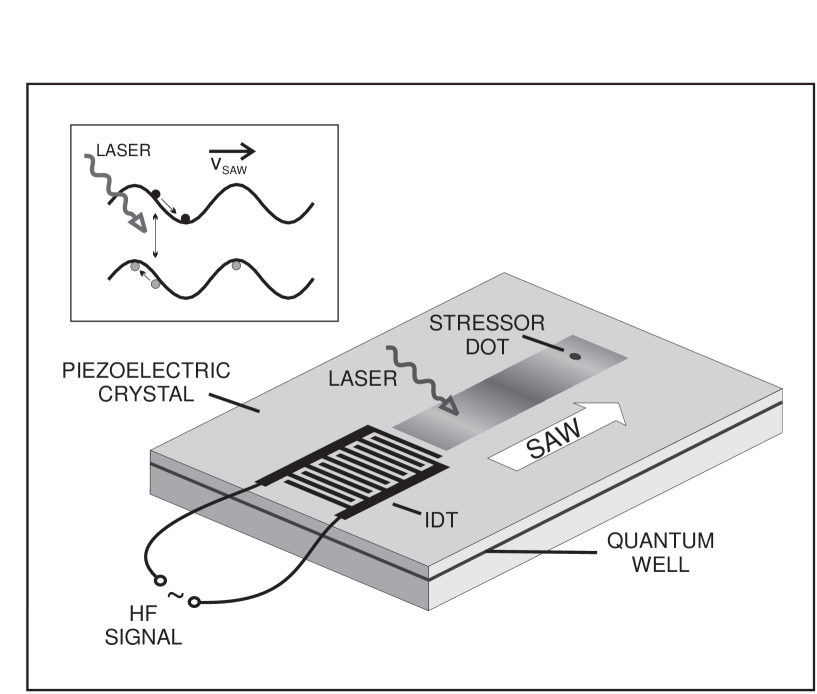
FIG. 1.: Schematic sketch of a SAW sample. The material of the system may be for example GaAs for the piezoelectric crystal, InGaAs for the quantum well and InP for the stressor. The inset depict the storage of optically generated excitons in the potential of the surface acoustic wave.

- [1] N.N. Ledentsov, V.A. Shchukin, M.Grundmann, N. Kirstaedter, J. Böhrer, O. Schmidt, D. Bimberg, V.M. Ustinov, A.Yu. Egorov, A.E. Zhukov, P.S. Kop’ev, S.V. Zaitsev, N.Yu. Gordeev, Zh.I. Alferov, A.I. Borovkov, A.O. Kosogov, S.S. Ruvimov, P. Werner, U. Gösele, and J. Heydenreich, Phys. Rev. B 54, 8743 (1996).
- [2] N. Kirstaedter, O.G. Schmidt, N.N. Ledentsov, D. Bimberg, V.M. Ustinov, A.Yu. Egorov, A.E. Zhukov, M.V. Maximov, P.S. Kop’ev, and Zh.I. Alferov, Appl. Phys. Lett. 69, 1226 (1996).
- [3] M. Grundmann and D. Bimberg, phys. stat. sol. (a) 164, 279 (1997).
- [4] M. Asada, Y. Miyamoto, and Y. Suematsu, IEEE J. Quantum Electron. 22, 1915 (1986).
- [5] H. Saito, K. Nishi, I. Ogura, S. Sugou, and Y. Sugimoto , Appl. Phys. Lett 69 3140 (1996).
- [6] H. Shoji, Y. Nakata, K. Mukai, Y. Sugiyama, M. Sugawara, N. Yokoyama, and H. Ishikawa, Jpn. J. Appl. Phys. 35, 903 (1996).
- [7] J.A. Lott, N.N Ledentsov, V.M. Ustinov, A.Yu. Egorov, A.E. Zhukov, P.S. Kop’ev, Zh.I. Alferov, and D. Bimberg, Electr. Lett. 33, 1150 (1997).
- [8] S. Machida, Y. Yamamoto, and Y. Itaya, Phys. Rev Lett. 58, 1000 (1987).
- [9] S. Machida and Y. Yamamoto, Phys. Rev. Lett 60, 792 (1988).
- [10] C. Rocke, S. Zimmermann, A. Wixforth, J.P. Kotthaus, G. Böhm, and G. Weimann, Phys. Rev. Lett. 78 4099 (1997), cond-mat/9704029
- [11] C. Rocke, A. Wixforth, J.P. Kotthaus, W. Klein, H.Böhm, and G. Weimann, Inst. Phys. Conf. Ser. 155, (IOP Publishing, Bristol, 1997), pp. 125-128, cond-mat/9609250
- [12] J.M. Shilton, V.I. Talyanskii, M. Pepper, D.A. Ritchie, J.E.F. Frost, C.J.B. Ford, C.G. Smith, and G.A.C. Jones, J. Phys.: Condens. Matter 8, 531 (1996).
- [13] Y. Yamamoto and S.Tarucha, Jpn. J. Appl. Phys. 31, 1198 (1992).
- [14] P. Filipowicz, J. Javanainen, and P. Meystre, Phys.Rev. A 34, 3077 (1986).
- [15] J. Bergou, L. Davidovich, M. Orszag, C. Benkert, M. Hillery, and M.O. Scully, Phys. Rev. A 40, 5073 (1989).
- [16] F. Haake, S.M. Tan, and D.F. Walls, Phys. Rev. A 40, 7121 (1989).
- [17] S.Y. Zhu, M.S. Zubairy, C. Su, and J.Bergou, Phys. Rev. A 45, 499 (1992).
- [18] R.P. Puri, F. Haake and D. Forster, J. Opt. Soc. Am. B 13, 2689 (1996).