Transitions in quantum networks

Abstract

We consider transitions in quantum networks analogous to those in the two-dimensional Ising model. We show that for a network of active components the transition is between the quantum and the classical behaviour of the network, and the critical amplification coincides with the fundamental quantum cloning limit.

Precise control over single quantum systems is essential in testing and harnessing of quantum mechanics. This has become possible with the advances in laser cooling and trapping techniques and manipulation of optical elements in the one-photon level. The availability of single quantum systems has fed the interest in quantum networks: A quantum computer [1] is a network of individual quantum systems, where any two of the nodes can interact with each other. Most quantum private communication schemes [2] are networks of two or three nodes. In addition to these information processing and communication related applications, networks of optical components [3] and avoided crossings in multilevel systems [4, 5] have been considered in order to study higher dimensional quantum interference effects.

According to statistical physics, a set of probabilistically behaving individual systems can exhibit critical behaviour when connected. In this paper we consider the question whether transition phenomena exist in networks of systems which behave probabilistically not because of finite temperature but due to their quantum nature; transitions are known to exist in Ising quantum chain models. We define a model of a quantum network which carries in its structure a formal analogy to the two-dimensional Ising model. Such networks can be experimentally realized by various active (energy-consuming) or passive (energy-preserving) components. It is found that transitions do take place and we are able to give them a clear physical interpretation. For active systems the transition is between quantum and classical, for passive systems between diabatic and adiabatic behaviour of the network. The transition phenomenon is clearly reflected in observable quantities.

The Ising model describes a set of two-state systems which interact with their nearest neighbours; a quantum analogy of such a setup can be experimentally realized in various ways, as will be explained below. Fig.1 shows schematically a 2-D quantum network with nearest neighbour interactions. To define the building blocks of this network we now take a closer look at the Ising model.

The two-state systems in the Ising model, let us say spins, are on a 2-D lattice of the size $N\times M$. Since only nearest neighbour interactions are taken into account, the total energy of the system can be expressed using the energy $E(\mu)$ of one column (with the spin configuration $\mu$) and the energy $E(\mu,\mu^{\prime})$ between two columns. Let $s_{k}=\pm 1$ denote the values of individual spins and $\epsilon$ be the absolute value of the energy of a spin-spin interaction. Then the energies can be written as $E(\mu)=-\epsilon\sum_{k=1}^{N}s_{k}s_{k+1}$ and $E(\mu,\mu^{\prime})=-\epsilon\sum_{k=1}^{N}s_{k}{s^{\prime}}_{k}$.

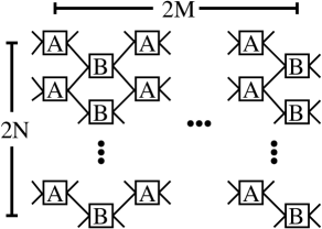
FIG. 1.: A quantum network where the nodes are connected to their nearest neighbours. The boxes A and B denote the transformations performed at the nodes; when they are defined by Eq.(1) the network has a relation to the Ising model.

The partition function $Q(T)$ can be expressed in a simple form by defining a $2^{N}\times 2^{N}$ matrix ${\cal P}$ whose matrix elements are the thermal weight factors corresponding to a particular spin configuration of two neighbouring columns $\langle\mu|{\cal P}|\mu^{\prime}\rangle\equiv e^{-\beta[E(\mu,\mu^{\prime})+E(\mu)]}$. With this notation $Q(T)=Tr{\cal P}^{M}=\sum_{\alpha=1}^{2^{N}}(\lambda_{\alpha})^{M}$. The eigenvalues $\lambda_{\alpha}$ thus determine the thermodynamics of the system. As was shown by Onsager and Kaufmann [6], the $2^{N}\times 2^{N}$ matrix ${\cal P}$ is a spinor representation of a set of plane rotations in $2N\times 2N$ dimensional space. The eigenvalues of ${\cal P}$ are uniquely determined by the eigenvalues of the corresponding plane rotation matrix $P$, which is

$$P=\left[\begin{array}[]{cccc}\framebox{A}&\begin{array}[]{cc}0&0\\ 0&0\end{array}&\begin{array}[]{c}\cdots\\ \cdots\end{array}&\\ \begin{array}[]{cc}0&0\\ 0&0\end{array}&\framebox{A}&&\\ \begin{array}[]{cc}\vdots&\vdots\end{array}&&\ddots&\\ &&&\framebox{A}\end{array}\right]\left[\begin{array}[]{ccccc}B_{22}&\begin{array}[]{cc}0&0\end{array}&\cdots&&B_{21}\\ \begin{array}[]{c}0\\ 0\end{array}&\framebox{B}&&&\\ \vdots&&\framebox{B}&&\\ &&&\ddots&\\ B_{12}&&&&B_{11}\end{array}\right]$$ (20)

where

$$\framebox{A}=\left[\begin{array}[]{cc}\cosh\theta&i\sinh\theta\\ -i\sinh\theta&\cosh\theta\end{array}\right] \framebox{B}=\left[\begin{array}[]{cc}\cosh\phi&i\sinh\phi\\ -i\sinh\phi&\cosh\phi\end{array}\right]$$ ; (25)

$$\coth\theta = \cosh\phi$$ (26)

and $\phi=2\epsilon/kT$.

The form of the matrix $P$ suggests immediately a quantum-network analogue. The matrices $A$ and $B$ can be interpreted to describe unitary evolution of a two-state or two-mode system. The matrix $P$ is then the evolution operator over a period in the network of Fig.1. The inputs of the network are mixed pairwise according to the transformation $A$, and then the pairs are let to interact with the neighbouring ones by applying the shifted set of operations $B$. By repeating this $M$ times, a $2N\times 2M$ dimensional network can be constructed [7]. Since $P$ contains all the physical information of the Ising model, e.g. the phase transitions, we may expect analogous phenomena in the quantum network described by $P$. Note that our aim is not to consider a set of quantized spin-systems at a finite temperature, like in the context of NMR quantum computing [8]. Instead, we borrow from the Ising model the abstract structure describing classical statistical behaviour, and ask what kind of quantum behaviour it could describe.

The physical realizations of the quantum network $P$ can be divided into two groups. When the angle $\phi$ is real, $A$ and $B$ are SU(1,1)-type matrices describing energy-consuming (active) operations. Imaginary $\phi$ leads to SU(2) matrices, which correspond to energy-preserving (passive) manipulations of the two modes or two states. Parametric amplifiers, four-wave mixers and phase-conjugating mirrors are SU(1,1) devices which can operate also in the quantum regime [9]: they could be used to build a network of active (quantum) optical components. The corresponding passive networks could be realized, for example, with beam splitters or fibre couplers. Also a network of intersecting energy levels can be described by a network of the type in Fig.1: the avoided crossings between the levels are identified with the operations $A$ and $B$. Corresponding physical systems are for instance Rydberg atoms [10] and longitudinal electro-magnetic modes in a cavity [4]. One can also consider the matrix $P$ as a set of operations done by a quantum computer [11]. For simplicity, in the following we call the SU(1,1) components amplifiers and the SU(2) components beam splitters, but actually mean any of the possible realizations.

Note that according to (26) $A\rightarrow I_{2}$ when the angle $\phi\rightarrow\infty$, and $B\rightarrow I_{2}$ when $\phi\rightarrow 0$. That is, in both of these limits the network decomposes into sets of non-interacting modes. Thus $P$ describes a quantum network where only nearest neighbours interact, and where a single parameter $\phi$ determines the relative importance of the interactions, i.e. the network character of the system.

The transitions in the network are determined by the eigenvalues of $P$. The only problem in diagonalizing $P$ is the relative shift between the sets of $A$ and $B$. This can be solved by the discrete Fourier transform $(F_{N})_{kl}=\exp(i2\pi kl/N)/\sqrt{N}\equiv\omega^{kl}/\sqrt{N}$, because the Fourier transform of the shift matrix $(S_{N})_{kl}=\delta_{k+1,l}+\delta_{kN}\delta_{l1}$ is diagonal: $F^{\dagger}_{N}S_{N}F_{N}=D_{\omega}$, where $(D_{\omega})_{kl}=\omega^{k-1}\delta_{kl}$. The whole network matrix $P$ thus decomposes into

$$P=I_{2}\otimes F_{N}\left[\begin{array}[]{ccc}\framebox{$K_{0}$}&0_{2}&\cdots\\ 0_{2}&\ddots&\\ \vdots&&\framebox{$K_{N-1}$}\end{array}\right]I_{2}\otimes F^{\dagger}_{N},$$ (30)

where

$$\framebox{$K_{n}$}=$$ (31)

$$\left[\begin{array}[]{cc}C(\theta)C(\phi)+S(\theta)S(\phi)\omega^{-n}&C(\theta)S(\phi)-C(\phi)S(\theta)\omega^{n}\\ -C(\theta)S(\phi)+C(\phi)S(\theta)\omega^{-n}&C(\theta)C(\phi)+S(\theta)S(\phi)\omega^{n}\end{array}\right]$$ (34)

and $C\equiv\cosh$ and $S\equiv i\sinh$. Most textbooks present the solution of the Ising model in a slightly different form, but we have formulated the problem as in (30) in order to make a connection to interferometers. The usual Mach-Zehnder interferometer affects the input states by a unitary transformation $U_{M-Z}$ which can be formally written as

$$U_{M-Z}=I_{1}\otimes F_{2}\left[\begin{array}[]{cc}K_{0}&0\\ 0&K_{1}\end{array}\right]I_{1}\otimes F_{2}^{\dagger},$$ (37)

where $K_{n}=\exp(i\phi n)$ is determined by a chosen phase $\phi$. Thus the Ising-type network we consider acts like an $N$-dimensional interferometer where, instead of one-mode phase shifts, two-mode rotations are performed in between the $N$-dimensional mixers $F_{N}$ and $F^{\dagger}_{N}$ [12].

From (31) one obtains the eigenvalues $e^{\pm\gamma_{n}}$, where $\gamma_{n}$ are determined via

$$\cosh\gamma_{n} = \cosh\theta\cosh\phi-\cos\left(\frac{2\pi n}{N}\right)\sinh\theta\sinh\phi$$ (38)

$$= \coth\phi\cosh\phi-\cos\left(\frac{2\pi n}{N}\right).$$ (39)

An explicit expression for $\gamma_{n}$ is given via the integral representation [6]

$$\gamma_{n}=\int_{0}^{\pi}\frac{d\nu}{\pi}\log\left[2\left(\coth\phi\cosh\phi-\cos\left(\frac{2\pi n}{N}\right)-\cos\nu\right)\right]$$ (40)

As can be seen from above, the zeroth eigenvalue ($n=0$) is not a smooth function of $\phi$: at $\gamma_{0}=0$, i.e. when $\cosh\phi=\sqrt{2}$, its derivative $\frac{d\gamma_{0}}{d\phi}$ has a discontinuity. In the Ising model this gives the transition temperature $kT_{c}=2.269\epsilon$. We are now at the point to interpret what this mathematical behaviour means physically in the case of quantum networks. We will first consider active SU(1,1) networks, then the passive SU(2) ones.

For the active SU(1,1) networks the amplification $G$ of the single components $A$ and $B$ is $\cosh^{2}\theta$ and $\cosh^{2}\phi$, respectively. The critical amplification $G_{c}=\cosh^{2}\theta_{c}=\cosh^{2}\phi_{c}=2$ has an interesting physical interpretation. It has been shown [13] that for parametric amplifiers $G=2$ sets a borderline between quantum and classical performance of the device. For $G\geq 2$ an initially squeezed input loses the squeezing, i.e. its non-classical properties in the process of amplification. This is sometimes called the ”magic cloning limit”; if it did not exist, one could reproduce quantum states, which would simply violate quantum mechanics. By considering what happens at the critical amplification point, as well as below and above it, we can show that $G_{c}$ coinciding with the ”magic cloning limit” is not a mere coincidence.

In the Ising model the transition point divides regimes of order and disorder. To see whether $G_{c}$ imposes any such boundary we consider again the matrices $K_{n}$, now written in the form

$$K_{n}=\cosh\phi\left[\begin{array}[]{cc}\coth\phi-\frac{\omega^{-n}}{\cosh\phi}&i-\frac{i\omega^{n}}{\sinh\phi}\\ -i+\frac{i\omega^{-n}}{\sinh\phi}&\coth\phi-\frac{\omega^{n}}{\cosh\phi}\end{array}\right].$$ (43)

In the limit $\phi\rightarrow 0$ the matrices $K_{n}$ are clearly functions of $\omega^{n}$, but when $\phi\rightarrow\infty$, they become increasingly independent of $n$; actually $G<2$ corresponds to the condition $|\omega^{n}|>|\sinh\phi|$. Considering Eq.(30) one sees that when the input is any vector (specified by $n$) of the Fourier transform matrix, i.e. of the type $1/\sqrt{N}[1,1,\omega^{n},\omega^{n},\omega^{2n},\omega^{2n}...]$, it will be affected by the corresponding $K_{n}$ matrix. For $G>>2$, however, the $K_{n}$ tend to be independent of $n$; this means that the network gives the same response independent of the relative phases $\omega^{n}$ of the input modes. The opposite is true for $G<2$. Thus the network behaves like a phase sensitive, i.e. a quantum device below $G_{c}=2$, and classically above it: it is logical that $G_{c}=2$ coincides with the quantum-classical border of the individual components.

Let us now consider the passive SU(2) networks [14]. The analogy to the Ising model is then not one-to-one. For example (26) is true only for one trivial choice for the, now imaginary, angle $\phi$. We can, however, define a network which has the same basic properties as the active ones: nodes connected by nearest neighbour interactions, with one parameter $\phi$ quantifying the importance of these interactions. Let us, for example, fix $\theta=i\pi/4$ and denote $\phi^{\prime}=-i\phi$. In the limits $\phi^{\prime}\rightarrow 0$ and $\phi^{\prime}\rightarrow\pi/2$ the network decomposes into sets of independent modes, while intermediate values of $\phi^{\prime}$ describe a network of interacting modes. The zeroth eigenvalue of the matrix $P$ is defined by the equation $\cos\gamma_{0}=\frac{1}{\sqrt{2}}(\cos\phi^{\prime}+\sin\phi^{\prime})$. It reaches the value zero for $\phi^{\prime}_{c}=\pi/4$, and its derivative with respect to $\phi^{\prime}$ has a singularity at this point. The transition thus takes place at the point when all the beam splitters are half-transmitting. Here it is, however, not a transition between quantum and classical regimes like in the case of active networks. Names for the two regimes separated by $\phi^{\prime}_{c}$ can be given by considering a network of avoided crossings. Imagine that in Fig.1 the individual elements are actually avoided crossings between intersecting energy levels. At each crossing the system can either follow the energy level adiabatically, or make a Landau-Zener transition to the neighbouring level, that is, to show diabatic behaviour. Indicating which of these processes is more likely, we call the regime $\phi^{\prime}<\pi/4$ diabatic and $\phi^{\prime}>\pi/4$ adiabatic. Thus we have shown that the system does not evolve smoothly from the adiabatic to the diabatic regime and vice versa, but exhibits at the critical transmittance $t_{c}=\frac{1}{2}$ a transition which is associated with singularities in the global parameters of the network.

We have now identified the regimes of behaviour separated by the transition, both for the SU(1,1) and SU(2) networks. The essential feature is the appearance of singularities at the transition point. In a normal situation the tuning of local parameters, that is the parameters of the network nodes such as beam splitters or amplifiers, leads to a smooth change in the global properties of the network. At the transition point this is not true. To demonstrate the observability of this phenomenon we now consider the response of the network in the case of two generic types of input states: the equal superposition of all modes, and the eigenstate of one mode.

The output of the network is given by the transformation $P^{M}$. The $M$th powers of $K_{n}$ in Eq.(30) can be obtained using the diagonalized form of (31): $(K_{n}^{M})_{11}=\cosh M\gamma_{n}+i\sin(2\pi n/N)\sinh M\gamma_{n}/\sinh\gamma_{n}=(K_{n}^{M})_{22}^{*}$ and $(K_{n}^{M})_{21}=(K_{n})_{21}\sinh M\gamma_{n}/\sinh\gamma_{n}=(K_{n}^{M})_{12}^{*}$. An input in an equal superposition state with a phase periodicity determined by $n$, that is, $[1,0,\omega^{n},0,\omega^{2n},...]/\sqrt{N}$, will be transformed into the output state $[(K_{n}^{M})_{11},(K_{n}^{M})_{12},\omega^{n}(K_{n}^{M})_{11},\omega^{n}(K_{n}^{M})_{12},...]/\sqrt{N}$. By choosing $n$ one can thus control constructive and destructive interference in the network ($\gamma_{n+1}>\gamma_{n}$). The choice $n=0$ is a special one: at $G_{c}$ $\gamma_{0}=0$ and the whole network becomes transparent. The transparency remains true independent of $M$; one may consider this to be analogous to the appearance of long range correlations at $T_{c}$ in the Ising model. Furthermore, for $n=0$ the transition is clearly manifested in the measurable output intensities. The global amplification coefficient is then simply $M\gamma_{0}$, and its rate of change with respect to the local amplification coefficient $\phi$, $M\frac{d\gamma_{0}}{d\phi}$, has a discontinuity at $G_{c}$. For an input in the eigenstate of the $2n+1$th mode, i.e. $[0,0,...,1,...,0]$, the $2n+1$th output amplitude has the form $\frac{1}{N}\sum_{m=0}^{N-1}\cosh M\gamma_{m}+i\sin(2\pi m/N)\sinh M\gamma_{m}/\sinh\gamma_{m}$. Since this sum contains all $\gamma_{m}$, the singularity is smoothed. By choosing the type of the input one can thus modify the manifestations of the transition in the output. Similar considerations can be carried out to find the fingerprints of the transition in the case of SU(2) networks.

Note that due to the non-smoothness of $\gamma_{0}$ operations defined by $G_{c}$ or $t_{c}$ may be unstable ones. This has interesting consequences: for instance, some operations to be performed by the proposed quantum computer may hit an unstable transition point of the whole system. Also quantum correlations and entanglement are expected to show special behaviour near the transition. Furthermore, it could be illuminating to consider higher dimensional quantum interference experiments in connection with the Ising model. The theoretical description of networks of avoided crossings [15, 5, 4] resembles the one presented here, with the choice $A=B$ and with the addition of extra phase factors due to free evolution of the system between the avoided crossings. However, when the free evolution phase factors are multiples of $\pi/N$, the system reduces to the one described here, up to trivial differences. It is interesting to note, that experimentally observed recurrence phenomena appear in these networks exactly for such values of the free evolution phase, that is, when the system reduces to an Ising-type network. Moreover, approximate analytical results predicting the recurrences are possible to derive in the adiabatic and diabatic limits [5], but not for the case of 50:50 crossings which according to our results is the transition point between these regimes.

In summary, we have taken a novel point of view to the networks used in quantum computation, communication and interference experiments: we have shown that they can exhibit transition phenomena. Although the individual quantum components at the network nodes are smoothly behaving, in certain network configurations — like the 2-D Ising model analogue considered here — they show non-smooth global behaviour. For networks based on active SU(1,1) components the transition is particularly interesting since the critical amplification $G_{c}=2$ coincides with the ’magic cloning limit’ above which an initially squeezed input loses its non-classical properties in the process of amplification. We have shown that the whole network too has regimes of quantum and classical behaviour: below the transition point $G_{c}=2$ the network is sensitive to the phase information in the input, for higher values of $G$ the output depends mainly on the intensities of the inputs. In the case of passive SU(2) networks the critical transmittance $t_{c}=\frac{1}{2}$ separates regions of adiabatic and diabatic behaviour. We have indicated how the transition is reflected in observable quantities.

Acknowledgements We thank Prof. B. Kaufmann, Prof. W. P. Schleich, Dr. I. Marzoli and Dr. D. Bouwmeester for interesting discussions, and Prof. P. Zoller for reading the manuscript and for useful comments.

REFERENCES

- [1] R. Feynman, Int. J. Theor. Phys. 21, 467 (1982); P. W. Shor, in Proceedings of the 35th Annual Symposium on the Foundations of Computer Science, ed. S. Goldwasser (IEEE Computer Society Press, Los Alamitos, CA, 1994), p.124.
- [2] A. Ekert, Phys. Rev. Lett. 67, 661 (1991); C. H. Bennett, Phys. Rev. Lett. 68, 3121 (1992).
- [3] M. Reck, A. Zeilinger, H. J. Bernstein, and P. Bertani, Phys. Rev. Lett. 73, 58 (1994); K. Mattle, M. Micheler, H. Weinfurter, A. Zeilinger, and M. Zukowski, Appl. Phys. B 60, S111 (1995).
- [4] D. Bouwmeester, I. Marzoli, G. Karman, W. P. Schleich, and J. P. Woerdman, submitted to Phys. Rev. A.
- [5] D. A. Harmin, Phys. Rev. A 56, 232 (1997).
- [6] L. Onsager, Phys. Rev. 65, 117 (1944); B. Kaufmann, Phys. Rev. 76, 1232 (1949); K. Huang, Statistical Mechanics (John Wiley & Sons, New York, 1987).
- [7] The networks should be either large enough, or imposed to periodic boundary conditions. In the case of optical components the latter can be easily realized.
- [8] N. A. Gerschenfeld and I. L. Chuang, Science 275, 350 (1997).
- [9] C. M. Caves, Phys. Rev. D 26, 1817 (1982), and references therein.
- [10] Rydberg States of Atoms and Molecules, edited by R. F. Stebbings and F. B. Dunning (CUP, Cambridge, 1983).
- [11] The first two-qubit gate has been realized with trapped ions [C. Monroe, D. M. Meekhof, B. E. King, W. M. Itano, and D. J. Wineland, Phys. Rev. Lett. 75, 4714 (1995)] according to the theoretical proposal in [J. I. Cirac and P. Zoller, Phys. Rev. Lett. 74, 4091 (1995)]. Other proposals utilize for example cavity QED techniques [T. Pellizzari, S. A. Gardiner, J. I. Cirac, and P. Zoller, Phys. Rev. Lett. 75, 3788 (1995); Q. A. Turchette, C. J. Hood, W. Lange, H. Mabuchi, and H. J. Kimble, Phys. Rev. Lett. 74, 4710 (1995)] and solid state structures [A. Barenco, D. Deutsch, A. Ekert, and R. Josza, Phys. Rev. Lett. 74, 4083 (1995)].
- [12] The Fourier transform matrices can be viewed as generalizations of balanced beam splitters () into higher dimensions, and can be efficiently constructed from two-dimensinal components with FFT-type procedures [P. Törmä, S. Stenholm, and I. Jex, Phys. Rev. A 52, 4853 (1995); H. Paul, P. Törmä, T. Kiss, and I. Jex, Phys. Rev. Lett. 76, 2464 (1996)].
- [13] S. Friberg and L. Mandel, Opt. Comm. 46, 141 (1983); R. Loudon and T. J. Shepherd, Optica Acta 31, 1243 (1984); S. Stenholm, Opt. Comm. 58, 177 (1986); U. Leonhardt, Phys. Rev. A 49, 1231 (1994).
- [14] Such networks are related to quantum cellular automata, see e.g. G. Grössing and A. Zeilinger, Complex Systems 2, 197 (1988); I. Bialynicki-Birula, Phys. Rev. D 49, 6920 (1994); D. A. Meyer, Phys. Rev. E 55, 5261 (1997) and references therein.
- [15] D. A. Harmin and P. N. Price, Phys. Rev. A 49, 1933 (1994); Yu. N. Demkov, P. B. Kurasov, and V. N. Ostrovsky, J. Phys. A: Math. Gen. 28, 4361 (1995).