Quantum Binary Decision for Driven Harmonic Oscillator

Abstract

We address the problem of determining whether or not a harmonic oscillator has been perturbed by an external force. Quantum detection and estimation theory has been used in devising optimum measurement schemes. Detection probability has been evaluated for different initial state preparations of oscillator. The corresponding lower bounds on minimum detectable perturbation intensity has been evaluated and a general bound for random phase perturbation has been also induced.

1 Introduction

The harmonic oscillator is a relatively simple model, which is widely utilized in many fields of physics. Indeed, it provides a satisfactory description of a large number of very different physical systems. This is true also in a quantum mechanical framework, where the harmonic oscillator plays a crucial role. Its spectrum of eigenvalues, in fact, is infinite, discrete and bounded from below, thus representing a paradigm for any bounded oscillating system.

Interesting physical features often comes with perturbation to harmonic behaviour, which are to be revealed from measurement performed on the system. This is the case, as an example, of oscillating electronic circuits [1] or of some large mass viewed as a gravitational antenna [2, 3, 4]. Also, a single mode radiation field is modeled on harmonic oscillator, and many optical devices act as driving terms in the dynamical evolution [5].

Quantum mechanically, different measurements lead to different informations about a physical system, as each observable shows up only an aspect of the state under examination [6, 7, 8]. Therefore, it is a matter of interest to analyze the different measurement processes, in order to find an optimized measurement scheme, which is capable to reveal perturbations as weak as possible. This project is a matter of quantum detection and estimation theory [9, 10], which regards the very general problem of extracting information on a physical system from measurement or a set of measurements.

In the present paper we address the binary decision theory for driven quantum harmonic oscillator. Let us consider an oscillator which is free to follow harmonic evolution, and possibly subjected to an external driving signal. After a fixed time $\tau$ we perform a measurement on the system, in order to check whether or not the oscillator has been perturbed. We are going to deal with two questions: first, which is the best measurement one can perform, in order to reveal perturbations as weak as possible with the minimum probability of error ? And second, which is the minimum detectable perturbation intensity, depending on the initial state preparation of the oscillator ?

We do not concern to any specific measurement device and we do not discuss the feasibility of optimized measurement. Rather, we attempt to derive a ultimate quantum limit on the detectable intensity of a perturbation, which depends only on the initial quantum state of the oscillator.

The paper will be organized as follows. In Section 2 we set the proper quantum measurement theory framework and illustrate the Neyman-Pearson strategy for binary decision. In Section 3 we consider different initial preparation states for the harmonic oscillator and derive the corresponding minimum detectable perturbation intensity. Section 4 closes the paper with some concluding remarks.

2 Quantum Detection Theory

2.1 Quantum measurements

In a quantum mechanical framework any measurement apparatus is a device, at least a mathematical one, which turns each quantum state $\hat{\rho}$ into a probability density distribution [11]

$$dP[\hat{\rho}]:\hat{\rho}\longrightarrow dP[\hat{\rho}](x)\qquad x\in{\cal X}\;,$$ (1)

where $\cal X$ is some measurable space, where the possible outcomes of the measurement lie. This can be the real Borel set or a subspace of it. The measurement map is provided by trace operation

$$dP[\hat{\rho}](x)=\hbox{Tr}\left\{\hat{\rho}\;d\hat{\mu}(x)\right\}\;,$$ (2)

which assures propagation of convex linear combinations from density operators toward probabilities. The above formula is the Born’s statistical rule [12]. It contains the whole probabilistic structure of quantum mechanics [13]. The Born rule leads to a genuine probability density distribution if the operator $d\hat{\mu}(x)$ satisfies the axioms for a probability operator measure (POM) [14], namely it is nonnegative

$$d\hat{\mu}(x)\geq 0\;,$$ (3)

and it provides a resolution of identity on the set of possible outcomes

$$\int_{\cal X}d\hat{\mu}(x)=\hat{\bf 1}\;.$$ (4)

Eq. (4) guarantees the probability density in Eq. (2) to be normalized, whereas positiveness of $d\hat{\mu}(x)$ also assures it is selfadjoint.

Spectral, orthogonal resolution $d\hat{E}(z)$ of a selfadjoint operator

$$\hat{Z}=\int_{\cal Z}z\;d\hat{E}(z) d\hat{E}(z)=|z\rangle\langle z|\;dz$$

$$\hat{Z}|z\rangle=z|z\rangle \langle z|z^{\prime}\rangle=\delta_{\cal Z}(z-z^{\prime})\;,$$ (5)

provides a projection valued measure (PVM) which belongs to the class of POM. However, this is not the most general example. Also nonorthogonal projectors or overcomplete sets provides POM, namely available measurement scheme [15, 16, 17].

It is worth noting that a POM is necessarily (Naimark Theorem) [18] a partial trace of a PVM coming from a selfadjoint operator defined on a larger Hilbert space. The latter can be thought as the whole Hilbert space describing both, the system under examinations and the measurement apparatus [19]. As we are not going to deal with physical implementation of measurement we can restrict our attention on the Hilbert space of the examined system only. Thus, any measurement is properly described by a POM.

2.2 Driven Harmonic Oscillator

The quantum mechanical description of harmonic oscillator is based on annihilation $a$ and creation $a^{{\dagger}}$ operators

$$a=\sqrt{\frac{m\omega}{2}}x+i\sqrt{\frac{1}{2m\omega}}p\;,$$ (6)

which form the number operator $\hat{N}=a^{{\dagger}}a$. Due to commutation relation $[a,a^{{\dagger}}]=1$, multiple applications of $a^{{\dagger}}$ to the vacuum state leads to the Fock basis $|n\rangle=(n!)^{-1/2}a^{{\dagger}n}|0\rangle$ which span the whole Hilbert space representing the possible levels of excitation for the oscillator. Number states represents also the eigenstates of the number operator, whose spectrum coincides with the set of the natural numbers ${\cal N}=0,1,...$. The eigenstates of annihilation operator $a|\alpha\rangle=\alpha|\alpha\rangle$ constitute the overcomplete set of coherent states, $\alpha$ being the complex amplitude of the harmonic oscillations. Coherent states can also be obtained from the vacuum by the action of displacement operator $\hat{D}(\alpha)=\exp\{\alpha a^{{\dagger}}-\bar{\alpha}a\}$ [20]

$$|\alpha\rangle = \hat{D}(\alpha)|0\rangle$$

$$\hat{D}(\alpha)\hat{D}(\alpha^{\prime}) = \hat{D}(\alpha+\alpha^{\prime})\exp\left\{\hbox{Im}(\alpha\alpha^{\prime})\right\}\;.$$ (7)

Let us consider the Hamiltonian (natural unit $\hbar=1$)

$${\bf H}=-\frac{1}{2m}\frac{d^{2}}{dx^{2}}+\frac{1}{2}m\omega^{2}x^{2}+F(t)x\;.$$ (8)

It describes a classical harmonic oscillator of mass $m$ and frequency $\omega$ subjected to a time dependent driving force. In terms of annihilation and creation operator the Hamiltonian could be written as [21]

$${\bf H}=\omega a^{{\dagger}}a+\frac{F(t)}{\sqrt{2m\omega}}(a^{{\dagger}}+a)\;.$$ (9)

Finally, we adopt interaction (Dirac) picture to obtain

$${\bf H}_{I}=\frac{F(t)}{\sqrt{2m\omega}}(a^{{\dagger}}+a)\;.$$ (10)

Let now consider the initial state of the oscillator to be $\hat{\rho}_{0}$. If no driving force is present the final state, after a fixed evolution time $\tau$, is still $\hat{\rho}_{0}$. Otherwise, we have

$$\hat{\rho}_{1}=\hat{U}\;\hat{\rho}_{0}\;\hat{U}^{{\dagger}}\;,$$ (11)

where the evolution operator $\hat{U}=\exp\left\{i{\bf H}_{I}\tau\right\}$ could be written as a displacement operator [22]

$$\hat{U}\equiv\hat{D}(z)=\exp\left\{za^{{\dagger}}-\bar{z}a\right\}\;,$$ (12)

where

$$z=\frac{i\gamma\tau}{\sqrt{2m\omega}}\;,\qquad\quad\gamma=\int_{0}^{\tau}dt\;e^{i\omega t}\;F(t)\;.$$ (13)

The quantity $z$ represents the complex amplitude of the driving signal, whereas $|z|^{2}$ denotes the energy intensity of the perturbation, expressed in unit of the oscillator quanta $\omega$.

2.3 Neyman-Pearson Strategy for Binary Decision

Our goal is to determine whether or not the system has been perturbed. For this purpose we adopt a detection scheme as in Fig. 1. After the initial preparation the harmonic oscillator is left free to evolve for a fixed time $\tau$. Then, some kind of measurement $d\hat{\mu}(x)$ is performed. Starting from the outcomes of such a measurement we have to infer which is the state of the system, in order to discriminate between the following two hypothesis:

• No perturbation has been occurred during the time interval $\tau$, true if we infer $\hat{\rho}_{0}$;

• The system has been perturbed during the time interval $\tau$, true if we infer $\hat{\rho}_{1}$.

We denote by $P_{01}$ the probability of wrong inference, namely that one of inferring ${\cal H}_{1}$ when ${\cal H}_{0}$ is true. In hypothesis testing formulation this is usually referred to as false alarm probability [23]. Conversely, we denote by $P_{11}$ the detection probability, that is the probability of inferring ${\cal H}_{1}$ when it is actually true.

Figure 1: outline of the detection scheme. The system is initially prepared in some fixed state and then it is left free to evolve. During the free evolution it could be subjected to an external driving signal. After a fixed time interval $\tau$ we perform some kind of measuremen on the system. From the outcome of such a measurement we have to infer which is the state of the system, in order to discriminate between the perturbation hypothesis and the null hypothesis.

Now, which is the best measurement to discriminate between $\hat{\rho}_{0}$ and $\hat{\rho}_{1}$ ?

If these two states are mutually orthogonal the problem has a trivial solution. It is a matter of measuring the observable for which $\hat{\rho}_{0}$ and $\hat{\rho}_{1}$ are eigenstates. However this is not our case, as displacing a state of the harmonic oscillator leads to a different kind of state. Only coherent states maintain their characteristic under displacement

$$\hat{D}(z)|\alpha\rangle = \hat{D}(z)\hat{D}(\alpha)|0\rangle=\exp\left(\hbox{Im}[\alpha\bar{z}]\right)|\alpha+z\rangle\;.$$ (14)

However, coherent states constitute a nonorthogonal, overcomplete set by themselves. Thus, the above procedure cannot be applied in the present case, even for special initial states of the oscillator.

In the following we consider nonorthogonal $\hat{\rho}_{0}$ and $\hat{\rho}_{1}$ and we focus our attention on oscillator initially prepared in a pure state $\hat{\rho}_{0}=|\psi_{0}\rangle\langle\psi_{0}|$. As it can easily checked from Eq. (11) this means that also the perturbed state is a pure state $\hat{\rho}_{1}=|\psi_{1}\rangle\langle\psi_{1}|$.

The optimization problem can be analytically solved, for pure states, by adopting, the Neyman-Pearson criteria for binary decision [24]. The latter reads as follows. First, we have to fix a value for the false alarm probability $P_{01}$. Then, we have to find the measurement strategy $d\hat{\mu}(x)$ which maximizes the detection probability $P_{11}$. As a general definition, each measurement strategy which maximizes the detection probability $P_{11}$ for a fixed value of false alarm probability $P_{01}$ is considered as a Neyman-Pearson optimized detection for binary hypothesis testing. It was shown by Helstrom [9] and Holevo [10] that this very general problem could be reduced to solving the eigenvalue problem for the operator

$$d\hat{\mu}(x|\lambda)=\hat{\rho}_{1}-\lambda\hat{\rho}_{0}\;,$$ (15)

which represents the optimized measurement scheme. In general it is a POM rather than a PVM. Nevertheless when, as it is here the case, the two signals are linearly independent it has been proved by Kennedy [25, 26] that the optimum detection is described by a PVM. The parameter $\lambda$ is a Lagrange multiplier. Different values of $\lambda$ correspond to different values of the false alarm probability, namely to a different Neyman-Pearson strategies.

Once the eigenvalues problem for $d\hat{\mu}(x|\lambda)$ has been solved it results that only positive eigenvectors contribute to the detection probability $P_{11}$ [9, 27, 28]. Thus the decision strategy is transparent: after a measurement of the quantity $d\hat{\mu}(x|\lambda)$ if the outcome is positive we infer perturbation hypothesis ${\cal H}_{1}$ is true. Conversely, we infer null hypothesis ${\cal H}_{0}$ when obtaining negative outcome. By expanding the eigenstates of $d\hat{\mu}(x|\lambda)$ in terms of $|\psi_{0}\rangle$ and $|\psi_{1}\rangle$ Lagrange multiplier $\lambda$ can be eliminated from the expression of detection probability which results

$$P_{11}=\left\{\begin{array}[]{cr}\left[\sqrt{P_{01}\kappa}+\sqrt{(1-P_{01})(1-\kappa)}\right]^{2}&0\leq P_{01}\leq\kappa\\ &\\ 1&\kappa\leq P_{01}\leq 1\end{array}\right.\;.$$ (16)

In Eq. (16) $\kappa$ denotes the square modulus of the overlap between perturbed and unperturbed state of the harmonic oscillator, in formula $\kappa=|{\cal O}[\psi_{0},z]|^{2}$, where

$${\cal O}[\psi_{0},z]=\langle\psi_{0}|\psi_{1}\rangle=\langle\psi_{0}|\hat{D}(z)|\psi_{0}\rangle\;.$$ (17)

The overlap depends both on the initial state and on the perturbation amplitude. In the next Section we evaluate the quantity in Eq. (17) for relevant kinds of initial state.

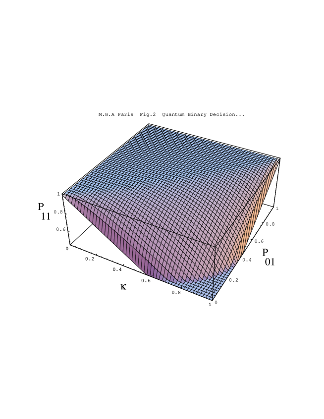
Figure 2: Three dimensional plot of the detection probability $P_{11}$ for Neyman-Pearson optimized detections as a function of the false alarm probability $P_{01}$ and the overlap $\kappa$ between the initial state and the perturbed one.

In Fig. 2 we report the detection probability of optimized detection strategies as a function of the false alarm probability $P_{01}$ and the overlap strength parameter $\kappa$. It is obvious that if the overlap is small, it is easy to discriminate between the two states. Thus, it is possible to obtain strategies with large detection probability without paying the price of an also large false alarm probability. On the contrary, if the overlap becomes appreciable it is difficult to discriminate the states. In the limit of complete overlap the perturbed and the unperturbed states become indistinguishable. Detection probability is now equal to false alarm probability and the decision strategy is just a matter of guessing after each random measurement outcome.

Choosing a value for the false alarm probability is a matter of convenience, depending on the specific problem this approach would be applied. The maximum tolerable value for $P_{01}$ increases with the expected number of measurement outcomes, and conversely a very low rate detection scheme needs a very small false alarm probability.

3 Quantum Binary Decision for Harmonic Oscillator

Once an acceptable value of false alarm probability has been fixed and the oscillator has been prepared in some initial state $|\psi_{0}\rangle$, the detection probability $P_{11}$ depends only on the perturbation intensity. A wise inference could be performed only when $P_{11}(z)\geq 1/2$, as only in this case the record $X=\{x_{0},x_{1},...,x_{N}\}$ of experimental data contain usable information. Thus, the threshold value $P_{11}(z)=1/2$ defines the minimum detectable perturbation for the so-prepared oscillator plus detector system. We will consider the intensity of the minimum detectable perturbation as the relevant parameter and we denote it by $|z_{min}|^{2}={\cal M}$. In the following Subsections we study the behaviour of $\kappa$ and ${\cal M}$ for different initial preparation $|\psi_{0}\rangle$.

3.1 Coherent States

For the oscillator prepared in a coherent state $|\alpha\rangle$ the overlap is given by

$${\cal O}[\alpha,z]=\langle\alpha|\hat{D}(z)|\alpha\rangle=\exp\{-\frac{1}{2}|z|^{2}\}\exp\{z\bar{\alpha}-\alpha\bar{z}\}\;,$$ (18)

and thus the overlap strength does not depend on the amplitude of the prepared coherent state

$$\kappa=\exp\{-|z|^{2}\}\;.$$ (19)

For zero false alarm probability the detection probability is given by $P_{11}(z)=1-\exp\{-|z|^{2}\}$. When a small false alarm probability is set ($P_{01}\leq\kappa$) the minimum detectable perturbation intensity is obtained by the inversion of the formula

$$\frac{1}{2}=\left[\sqrt{P_{01}\kappa}+\sqrt{(1-P_{01})(1-\kappa)}\right]^{2}\;,$$ (20)

that is,

$${\cal M}=\log\left(\frac{2}{1+\sqrt{P_{01}(1-P_{01})}}\right)\;.$$ (21)

The minimum detectable intensity is independent on the initial coherent amplitude. Thus coherent states provide a stable oscillating system, however also difficult to monitor in its fluctuations.

3.2 Squeezed States

Uncertainty principle set a lower bound for the product of fluctuations for two conjugated quantity. This implies a degree of freedom, namely that one can arbitrarily reduce the fluctuations in some variable upon increasing the fluctuations in the conjugated one. Indeed, squeezed states of the harmonic oscillator have been introduced as minimum uncertainty state for amplitude quadrature operators $\hat{x}_{\varphi}\propto a^{{\dagger}}e^{i\varphi}+ae^{-i\varphi}$ with phase dependent fluctuations.

Squeezed state can be obtained by the coherent displacement of squeezed vacuum $|\alpha,\zeta\rangle=\hat{D}(\alpha)|0,\zeta\rangle$ [29, 30]. The latter is obtained from the vacuum by the action of squeezing operator $|0,\zeta\rangle=S(\zeta)|0\rangle$, where

$$S(\zeta)=\exp\left\{\frac{1}{2}\left[\zeta a^{{\dagger}2}-\bar{\zeta}a^{2}\right]\right\}\;,$$ (22)

and $\zeta=r\exp\{i2\psi\}$, with $r$ real. Squeezing a state implies the introduction of some energy. The mean excitation number of a squeezed vacuum is given by $\bar{n}_{sq}\equiv\langle\zeta,0|\hat{N}|0,\zeta\rangle=\sinh^{2}r$.

As we have seen just above coherent amplitude does not cause any effect when subjected to displacement action. Therefore, we restrict our attention to squeezed vacuum $|0,\zeta\rangle$ which shows all the interesting phase dependent features related to squeezing. We also consider, for simplicity, a squeezed vacuum with squeezing phase equal to zero $\psi=0$.

The overlap is given by

$${\cal O}[r,z]=\exp\left\{-\frac{1}{2}|z|^{2}\left[\cosh 2r-\sinh 2r\cos^{2}\varphi\right]\right\}\;,$$ (23)

where $\varphi\equiv\arg(z)$ is the phase of the perturbation. In Fig. 3 we report the overlap (23) for a unit intensity perturbation $|z|^{2}=1$ as a function of the squeezing parameter $r$ and the perturbation phase $\varphi$. In the two limiting cases $\varphi=0,\pi/2$ we have, for the overlap strength

$$\kappa_{0}=\exp\left\{-2|z|^{2}\left[\bar{n}_{sq}+\frac{1}{2}-\sqrt{(\bar{n}_{sq}+1)\bar{n}_{sq}}\right]\right\}$$ (24)

$$\kappa_{\pi/2}=\exp\left\{-|z|^{2}\left[2\bar{n}_{sq}+1\right]\right\}\;.$$ (25)

However, the perturbation phase is reasonably random, or unknown. Thus, a relevant parameter to be considered is also the phase averaged overlap strength which is defined by

$$\bar{\kappa}=\left|\int_{\pi}^{\pi}\frac{d\varphi}{2\pi}\;{\cal O}[r,|z|e^{i\varphi}]\right|^{2}\;.$$ (26)

Inserting Eq. (23) in Eq. (26) leads to

$$\bar{\kappa} = \exp\left\{-|z|^{2}\left[2\bar{n}_{sq}+1-\sqrt{(\bar{n}_{sq}+1)\bar{n}_{sq}}\right]\right\}\times$$ (27)

$$\times \left[I_{0}\left(\frac{1}{2}|z|^{2}\sqrt{(\bar{n}_{sq}+1)\bar{n}_{sq}}\right)\right]^{2}\;,$$

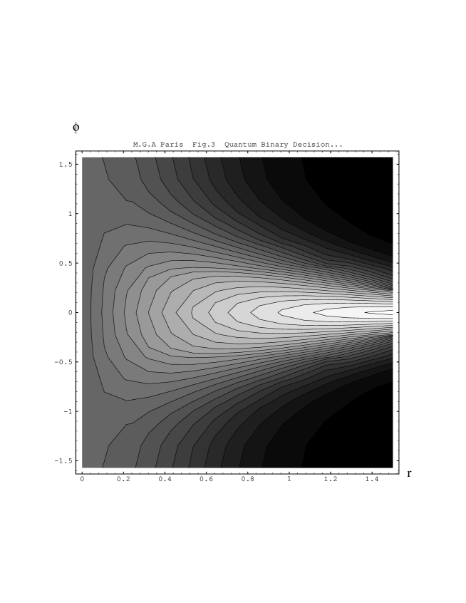
Figure 3: Contour plot of the overlap for the oscillator initially prepared in a squeezed vacuum. A perturbation with unit intensity is considered and the overlap is reported as a function of the squeezing parameter $r$ and the phase $\varphi$ of the perturbation.

with $I_{0}(x)$ denoting a modified Bessel function of the first kind [31].

The minimum perturbation equation (20) can be analytically solved for a fixed value of perturbation phase. We obtain

$${\cal M}_{0}=\log\left(\frac{2}{1+\sqrt{P_{01}(1-P_{01})}}\right)\exp\{2r\}\;,$$ (28)

where $e^{2r}=2\bar{n}_{sq}+1+2\sqrt{(\bar{n}_{sq}+1)\bar{n}_{sq}}$, and

$${\cal M}_{\pi/2}=\log\left(\frac{2}{1+\sqrt{P_{01}(1-P_{01})}}\right)\frac{1}{2\bar{n}_{sq}+1}\;.$$ (29)

From Eqs. (28) and (29) is apparent the strong effect of phase matching. When both phases, the perturbation one and the squeezing one, have the same value the overlap is strongly enhanced and thus the minimum detectable intensity increase (roughly linearly) with the increasing of the squeezing energy. On the contrary when the two phases are maximally mismatched, the overlap decreases with increasing energy of the initial states. Thus, the system becomes more and more sensitive to perturbation and minimum detectable intensity shows an inverse scaling with the initial preparation energy.

Figure 4: The minimum detectable perturbation intensity ${\cal M}$ for the oscillator initially prepared in a squeezed vacuum and random phase perturbation. The behaviour of ${\cal M}$ is reported as a function of the mean excitation number $\bar{n}_{sq}=\sinh^{2}r$ of the squeezed vacuum for different values of the false alarm probability $P_{01}$. The curves are clearly distinguishable in the region $\bar{n}_{sq}\sim 1$ where we have, from top to bottom, the behaviour for $P_{01}=0.00,0.01,0.02,0.05$ respectively.

In the case of random (unknown) phase we have not been able to solve analytically the perturbation equation. We solved it numerically. In Fig. 4 we report the behaviour of $\cal M$ as a function of $\bar{n}_{sq}$ for various values of the false alarm probability. For $\bar{n}_{sq}\geq 10$ the numerical results are very well interpolated by the formula

$${\cal M}\stackrel{{\scriptstyle\bar{n}_{sq}\geq 10}}{{\simeq}}\log\left(\frac{2}{1+\sqrt{P_{01}(1-P_{01})}}\right)\frac{1}{\bar{n}_{sq}}\;.$$ (30)

3.3 Number States

The overlap of a number state with its displaced version is a real number, thus the overlap strength $\kappa$ is just the square of the overlap ${\cal O}[n,z]$. We have

$$\kappa=\exp\{-|z|^{2}\}L_{n}^{2}(|z|^{2})\;,$$ (31)

where $L_{n}(x)$ denotes a Laguerre polynomials [31]. Number states are a phase insensitive kind of states. Therefore, preparing the harmonic oscillator in such a way is equivalent to a phase averaging by default.

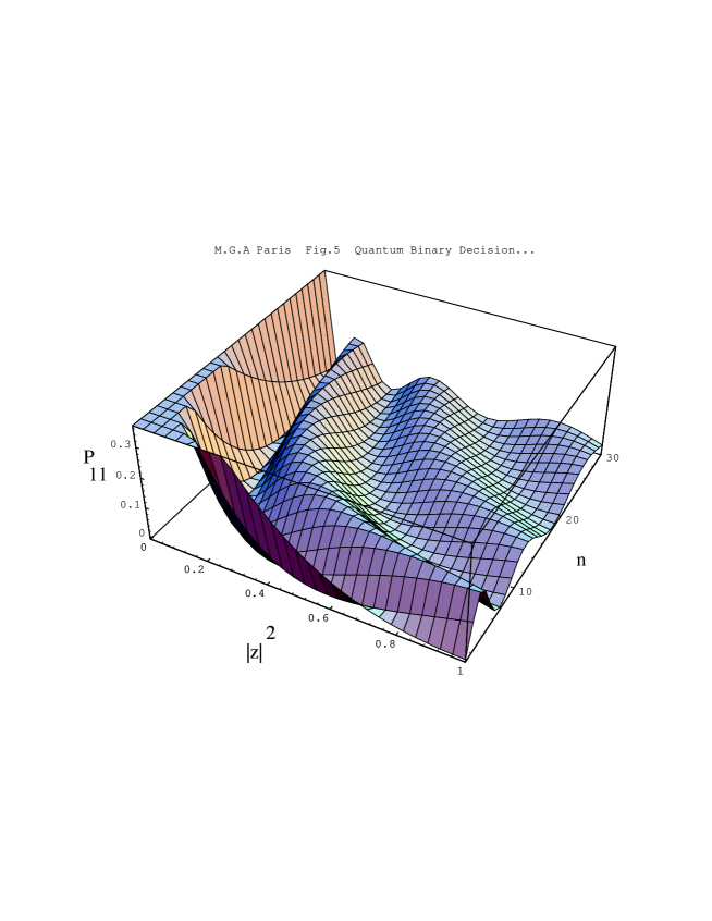
Figure 5: Three dimensional plot of the overlap strength $\kappa$ for the oscillator initially prepared in a number state. The overlap strength is reported as a function of the number $n$ and the perturbation intensity $|z|^{2}$.

In Fig. 5 we report the overlap strength as a function of the perturbation intensity and the excitation number of harmonic oscillator.

The minimum perturbation equation (20) reads as follows

$$\frac{1}{2}=\exp\{-{\cal M}\}L_{n}^{2}({\cal M})\;.$$ (32)

It could be numerically solved. Minimum detectable intensity scales as

$${\cal M}\stackrel{{\scriptstyle n\gg 1}}{{\simeq}}\frac{A}{n}\;,$$ (33)

with the proportionality constant depending on the value of the false alarm probability. Roughly we have

$$A\approx 0.3-\frac{3}{2}P_{01}\;.$$ (34)

3.4 Superposition of Coherent States

We end this section by dealing with superposition states. We consider an analytically solvable case which is provided by superpositions of coherent states. Let us introduce the two set of states expressed by

$$|\psi_{\pm}\rangle=\frac{1}{2\sqrt{1\pm\exp\{-2|\alpha|^{2}\}}}\left(|\alpha\rangle\pm|-\alpha\rangle\right)\;,$$ (35)

where $|\alpha\rangle$ denotes a coherent state. These states are known also as even and odd Schröedinger cats [32] as they are superposition states containing only even and odd number components respectively. The evaluation of the overlap can be carried out by means of the operatorial relations

$$\hat{D}(-\alpha)\hat{D}(z)\hat{D}(\alpha) = \exp\{\bar{z}\alpha-\bar{\alpha}z\}\hat{D}(z)$$

$$\hat{D}(\alpha)\hat{D}(z)\hat{D}(\alpha) = \hat{D}(z+2\alpha)\;.$$ (36)

We consider for simplicity $\alpha$ as a real number, thus we obtain

$${\cal O}[\alpha,\pm,z] = \frac{\exp\{-\frac{1}{2}|z|^{2}\}}{1\pm\exp\{-2\alpha^{2}\}}\Big{[}\cos\left(2\alpha|z|\sin\varphi\right)$$ (37)

$$\pm e^{-2\alpha^{2}}\cosh\left(2\alpha|z|\cos\varphi\right)\Big{]}\;,$$

being $\varphi$ the perturbation phase. After some calculations we arrive at the overlap strength for the fixed value $\varphi=0,\pi/2$ and for the phase averaged case. We have

$$\kappa_{0}^{\pm} = \frac{\exp\{-|z|^{2}\}}{(1\pm 2\exp\{-2\alpha^{2}\})^{2}}\times$$ (38)

$$\times \Big{[}1\pm\exp\{-2\alpha^{2}\}\cosh\left(2\alpha|z|\right)\Big{]}^{2}\;,$$

$$\kappa_{\pi/2}^{\pm} = \frac{\exp\{-|z|^{2}-4\alpha^{2}\}}{(1\pm 2\exp\{-2\alpha^{2}\})^{2}}\times$$ (39)

$$\times \Big{[}1\pm\exp\{2\alpha^{2}\}\cos\left(2\alpha|z|\right)\Big{]}^{2}\;,$$

$$\bar{\kappa}^{\pm} = \frac{\exp\{-|z|^{2}\}}{(1\pm 2\exp\{-2\alpha^{2}\})^{2}}\times$$ (40)

$$\times \Big{[}J_{0}\left(2\alpha|z|\right)\pm\exp\{-2\alpha^{2}\}I_{0}\left(2\alpha|z|\right)\Big{]}^{2}\;,$$

being $J_{0}(x)$ and $I_{0}(x)$ the Bessel function and the modified Bessel function of the first kind [31]. Notice that the mean excitation numbers for the superposition states are given by

$$\bar{n}_{\pm}=|\alpha|^{2}\frac{1\mp e^{-2|\alpha|^{2}}}{1\pm e^{-2|\alpha|^{2}}}\;.$$ (41)

The strong effect of phase matching is again apparent. The minimum perturbation equation can be solved in the asymptotic region of large excitation numbers, leading to the energy scaling

$${\cal M}_{0}^{\pm}\stackrel{{\scriptstyle\bar{n}_{\pm}\gg 1}}{{\propto}}\bar{n}_{\pm}\;,$$ (42)

$${\cal M}_{\pi/2}^{\pm}\stackrel{{\scriptstyle\bar{n}_{\pm}\gg 1}}{{\propto}}\frac{1}{2\bar{n}_{\pm}}\;,$$ (43)

$${\cal M}_{rnd}^{\pm}\stackrel{{\scriptstyle\bar{n}_{\pm}\gg 1}}{{\propto}}\frac{1}{\bar{n}_{\pm}}\;.$$ (44)

In the case of random phase perturbation the minimum detectable intensity shows, at least asymptotically, an inverse scaling relative to the mean excitation number of the initial state. The same behaviour we have observed for squeezed vacuum and number state initial preparation, and this seems to indicate a general bound for detectability of perturbations. Actually, the minimum detectable intensity ${\cal M}$ becomes almost independent on the initial preparation in the limit of high excitation numbers.

4 Conclusions

Quantum detection and estimation theory has been applied in binary hypothesis testing, regarding possible perturbations on harmonic behaviour of a physical system. The action of an external driving signal is described by a displacement operator, thus excluding the possibility that the perturbed state of the oscillator could be orthogonal to that has been initially prepared.

The detection probability has been evaluated, for different initial preparation of the oscillator, as a function of the perturbation intensity and the initial preparation energy. Minimum detectable perturbation intensities have been also evaluated, which represent the ultimate quantum limit in detecting a perturbation for fixed initial preparation of the harmonic oscillator. The lower bounds on detectable perturbation show a strong dependence on the phase matching. In-phase perturbations could be effectively detected only for weakly excited oscillators, as minimum detectable intensity linearly increases with initial energy. On the contrary, out-of-phase perturbations are easily detected also for high excitations. In the realistic case of random phase perturbation, the minimum detectable perturbation intensity seems to become independent on the initial preparation, at least in the asymptotic regime of large initial energy. This suggests that the inverse scaling ${\cal M}\propto\bar{n}^{-1}$ relative to the initial mean energy could be a general bound.

An ultimate quantum limit for detection of perturbations could be defined independently from initial preparation, upon a further optimization over all the possible quantum states of the oscillator.

References

- [1] C. W. Helstrom, Int. J. Theor. Phys. 1, 37 (1968).
- [2] J. Weber, Phys. Rev. 117, 306 (1960).
- [3] J. N. Hollenhorst, Phys. Rev. D19, 1669 (1979).
- [4] R. S. Bondurrant, J. H. Shapiro, Phys. Rev. D30, 2548 (1984).
- [5] L. Mandel, E. Wolf Optical Coherence and Quantum Optics, (Cambridge University Press, 1995).
- [6] S. Stenholm, Ann. Phys. (N.Y) 218, 233 (1992).
- [7] M. G. A. Paris, Phys. Rev. A53, 2658 (1996).
- [8] M. G. A. Paris, Opt. Comm. 124, 277 (1996).
- [9] C. W. Helstrom, Quantum Detection and Estimation Theory, (Academic, New York, 1976).
- [10] A. S. Holevo, Probabilistic and Statistical Aspect of Quantum Theory, (North-Holland, Amsterdam, 1982).
- [11] M. Ozawa, Operator algebras and nonstandard analysis in Current Topics in Operator Algebras ed. by H. Araki et. al., World Scientific, (Singapore 1991) p.52.
- [12] A. Bohm, The rigged Hilbert space and Quantum mechanics, (Springer, Berlin, 1978).
- [13] P. Busch, P. J. Lahti, Riv. Nuovo Cim. 18, 1 (1995).
- [14] W. Mlak, Hilbert Spaces and Operator Theory, (Kluwer Academic, Dordrecht, (1991).
- [15] C. W. Helstrom, Found. Phys. 4 453 (1974); Int. J. Theor. Phys. 11, 357 (1974).
- [16] N.G. Walker, J.E. Carrol, Opt. Quantum Electr. 18, 355 (1986); N. G. Walker, J. Mod. Opt. 34, 15 (1987).
- [17] G. M. D’Ariano, M. G. A. Paris, Phys. Rev. 49 3022 (1994).
- [18] M. A. Naimark, Izv. Akad. Nauk SSSR Ser.Mat. 4, 227 (1940); see also Ref. [14].
- [19] G. M. D’Ariano, M. G. A. Paris, Phys. Rev. A48 R4039 (1993).
- [20] K. E. Cahill, R. J. Glauber, Phys. Rev. 177, 1857 (1969); 177, 1882 (1969).
- [21] W. H. Louisell, Quantum Statistical properties of Radiation, (Wiley, 1973).
- [22] M. G. A. Paris, Phys. Lett. A217, 78 (1996).
- [23] E. L. Lehmann, Testing Statitstical Hypothesis, (Wiley, New York, 1959).
- [24] J. Neyman, E. Pearson, Proc. Camb. Phil. Soc. 29, 492 (1933); Phil. Trans. Roy. Soc. London A231, 289 (1933).
- [25] R. S. Kennedy, Mass. Inst. Tech. Res. Lab. Electron. Quart. Prog. Rep. 113 142 (1973).
- [26] M. Osaki, M. Ban, O. Hirota, Phys. Rev. A54 1691 (1996).
- [27] A. S. Holevo, J. Multivar. Anal. 3, 337 (1973).
- [28] H. P. Yuen, R. S. Kennedy, M. Lax, IEEE Trans. Inf. Theory, IT21, 125 (1975).
- [29] D. Stoler, Phys. Rev. D1, 3217 (1970); Phys. Rev. D4, 1925 (1971).
- [30] H. P. Yuen, Phys. Lett. A51, 1 (1975); Phys. Rev. A13, 2226 (1976).
- [31] I. S. Gradshteyn, I. M. Ryzhik, Table of integral, series, and product, (Academic Press, 1980).
- [32] S. Haroche, M. Brune, J.-M. Raimond, L. Davidovich in Fundamentals of Quantum Optics II, F. Ehlotzky ed., Lect. Notes in Phys. 420, (Springer, Berlin 1993).