A two-step optimized measurement for the phase-shift

Abstract

A two-step detection strategy is suggested for the precise measurement of the optical phase-shift. In the first step an unsharp, however, unbiased joint measurement of the phase and photon number is performed by heterodyning the signal field. Information coming from this step is then used for suitable squeezing of the probe mode to obtain a sharp phase distribution. Application to squeezed states leads to a phase sensitivity scaling as $\Delta\varphi\simeq N^{-1}$ relative to the total number of photons impinged into the apparatus. Numerical simulations of the whole detection strategy are also also presented.

1 Introduction

As a matter of fact, no hermitian operator describing the optical phase can be defined on the sole Hilbert space of a single mode radiation field. Nonetheless, measurements of the phase-shift have been experimentally carried out for quantized field [1, 2]. Moreover, different experimental setups produce different phase distributions when investigating the same state of radiation [3]. The contradiction among these facts is only apparent. Indeed, what is actually measured in physical experiments is always a phase difference between the signal mode and a reference mode, which represents the probe of the measuring device. This probe mode is also a quantized field, characterized by its own field (phase and amplitude) fluctuations. Therefore, it appears rather obvious that the resulting phase distribution could show dramatically different features upon different probe modes. In this paper we are going to take advantage of this fact in order to obtain an optimized measurement for the phase-shift. This means a detection scheme leading to a phase distribution as sharp as possible, provided that the physical constraint of a fixed amount of energy impinged into the apparatus is satisfied.

In the next section we briefly review the main features of generalized phase-space functions, whereas the two-step measurement scheme is analyzed in details in Section 3. In Section 4 a numerical simulation of the whole detection strategy is presented, in order to confirm the effectiveness of the method also for low excited states. Section 5 closes the paper with some concluding remarks.

2 Measuring generalized phase-space distributions

We are considering here a generic two-photocurrent device, namely an apparatus jointly measuring the real $\widehat{Z}_{1}$ and the imaginary $\widehat{Z}_{2}$ parts of the complex photocurrent $\widehat{Z}=\hat{a}+\hat{b}^{{\dagger}}$. The operators $\hat{a}$ and $\hat{b}$ describe two single modes of the radiation field. We refer to $a$ as the signal mode and to $b$ as the probe mode of the device. Such kind of devices are readily available in quantum optics. Examples are provided by the heterodyne detectors [4], the eight-port homodyne detectors [5] and the recently introduced six-port homodyne detectors [6].

Each random experimental outcome is represented by a couple of real numbers $(z_{1},z_{2})$ which can be viewed as a complex number $z$ on the plane of the field amplitude (phase-space) [7] . These are distributed according to a generalized phase space distribution [8, 9]

$$K_{b}(\alpha,\bar{\alpha})=\int_{\bf C}\frac{d^{2}\gamma}{\pi^{2}}\>e^{\bar{\gamma}\alpha-\gamma\bar{\alpha}}\>\Xi(\gamma,\bar{\gamma})\>,$$ (1)

which is the Fourier transform of the characteristic function

$$\Xi(\gamma,\bar{\gamma})=\hbox{Tr}\left\{\hat{\varrho}\>\exp\left[\bar{\gamma}\widehat{Z}-\gamma\widehat{Z}^{{\dagger}}\right]\right\}\>,$$ (2)

$\hat{\varrho}$ being the global density matrix describing both the modes $a$ and $b$. Here, we consider the probe mode to be independent on the signal mode, so that the input mode is factorized as $\hat{\varrho}=\hat{\varrho}_{a}\otimes\hat{\varrho}_{b}$. In this case the characteristic function $\Xi(\gamma,\bar{\gamma})$ can be written as a product

$$\Xi(\gamma,\bar{\gamma})=\hbox{Tr}\left\{\hat{\varrho}_{a}\otimes\hat{\varrho}_{b}\;\;\hat{D}_{a}(\gamma)\otimes\hat{D}_{b}(-\gamma)\right\}=\chi_{a}(\gamma,\bar{\gamma})\;\chi_{b}(-\gamma,-\bar{\gamma})\>,$$ (3)

being $\hat{D}_{a}(\gamma)=\exp\left[\gamma\hat{a}^{{\dagger}}-\bar{\gamma}\hat{a}\right]$ the displacement operator and

$$\chi_{i}(\gamma,\bar{\gamma})=\hbox{Tr}\left\{\hat{\varrho}\>\hat{D}_{i}(\gamma)\right\}\qquad i=a,b\,;$$

the single-mode characteristics function. The latter enters in the definition of the Wigner function of a single-mode radiation field

$$W_{i}(\alpha,\bar{\alpha})=\int_{\bf C}\frac{d^{2}\lambda}{\pi}\>\chi_{i}(\lambda,\bar{\lambda})\>\exp\left\{\bar{\lambda}\alpha-\lambda\bar{\alpha}\right\}\qquad i=a,b\;.$$ (4)

We now insert Eq. (3) into Eq. (1). By means of Eq. (4) and using the convolution theorem, we arrive at the result

$$K_{b}(\alpha,\bar{\alpha}) = W_{a}(\alpha,\bar{\alpha})\star W_{b}(-\alpha,-\bar{\alpha})=$$ (5)

$$= \int_{\bf C}\frac{d^{2}\beta}{\pi^{2}}\;W_{a}(\alpha+\beta,\bar{\alpha}+\bar{\beta})\>W_{b}(\beta,\bar{\beta})$$

the symbol $\star$ denoting convolution. ¿From Eq. (5) it results that two-photocurrent devices allows filtering of the signal Wigner function according to the probe Wigner function. Therefore, they are powerful apparatus in order to manipulate and redirect quantum fluctuations.

3 A two-step measurement scheme for the phase-shift

The phase distribution in a two-photocurrent measurement scheme is defined as the marginal distribution of $K_{b}(\alpha,\bar{\alpha})$ integrated over the radius,

$$p(\varphi)=\int_{0}^{\infty}\!\rho\>d\rho\;K_{b}(\rho e^{i\varphi},\rho e^{-i\varphi})\>.$$ (6)

When the probe mode is left unexcited $\hat{\varrho}_{b}=|0\rangle\langle 0|$, the probability distribution $K_{b}(\alpha,\bar{\alpha})$ coincides with the customary Husimi $Q$-function $Q(\alpha,\bar{\alpha})=1/\pi\langle\alpha|\hat{\varrho}|\alpha\rangle$ of the signal mode. The resulting marginal phase distribution, as defined by Eq. (6), is given by [10, 11]

$$p_{Q}(\varphi) = \int_{0}^{\infty}\!\rho\>d\rho\;Q(\rho e^{i\varphi},\rho e^{-i\varphi})$$ (7)

$$= \frac{1}{2\pi}\sum_{n,m}\>\frac{\Gamma[1+\frac{m+n}{2}]}{\sqrt{n!m!}}\>\exp\{i(n-m)\varphi\}\>\langle n|\hat{\varrho}|m\rangle\>.$$

The probability $p_{Q}(\varphi)$ is an unsharp, however unbiased phase distribution. That is, it provides a reliable mean value for the phase but it is a broad distribution due to the intrinsic quantum noise introduced by the joint measurement [12]. The basic idea in the present two-step scheme is to use information coming from the measurement of $p_{Q}(\varphi)$ in order to suitably squeeze the probe mode in the subsequent measurement. In this way the noise is redirected to the ’useless’ direction of $K_{b}(\alpha,\bar{\alpha})$ resulting in the sharper phase distribution. This procedure is illustrated in Fig. 1 for a generic quantum state.

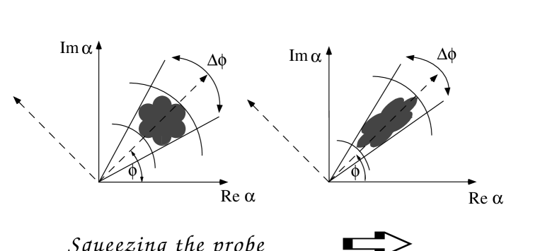
Figure 1: Manipulation of quantum fluctuations by squeezing of the probe mode. In (a) we show a generic, irregularly shaped, $Q$-function obtainable by two-photocurrent devices with vacuum probe mode. In (b) we show the distribution as obtained after squeezing the probe mode in the direction individuated by the mean value $\phi$ of the signal phase.

The natural choice for the state to apply this procedure is that of squeezed states

$$|\alpha,\zeta\rangle=\hat{D}(\alpha)\hat{S}(\zeta)|0\rangle\>,$$ (8)

being $\hat{S}(\zeta)=\exp\{1/2(\bar{\zeta}\hat{a}^{2}-\zeta\hat{a}^{{\dagger}2})\}$ the squeezing operator with complex parameter $\zeta=r\exp\{2i\psi\}$. Squeezed states, in fact, show phase-dependent field fluctuations and can be presently produced with reliable experimental techniques. The mean photon number is given by $\langle\hat{n}\rangle\equiv N=|\alpha|^{2}+\sinh^{2}r\equiv N_{coh}+N_{sq}$, where the coherent and squeezing contributions can be clearly distinguished. Squeezed states have been largely considered in interferometry, usually leading to high-precision measurements, though only for a special value of the phase-shift (the so-called working point of the interferometer) [13, 14]. Without loss of generality, we consider here a squeezed state with both coherent and squeezing phases equal to zero. This is accomplished by choosing $\alpha=x_{s}\in{\bf R}$ and $\zeta=r_{s}\in{\bf R}$.

In the first step of the measurement we leave the probe unexcited. The experimental outcomes are thus distributed according to the Husimi $Q$-function of a squeezed state which is a double Gaussian given by

$$Q(\alpha,\bar{\alpha})=\frac{1}{2\pi\sigma_{1}\sigma_{2}}\exp\left\{-\frac{[\hbox{Re}(\alpha)-x_{s}]^{2}}{2\sigma_{1}^{2}}-\frac{[\hbox{Im}(\alpha)]^{2}}{2\sigma_{2}^{2}}\right\},$$ (9)

$$\sigma_{1}^{2}=\frac{1}{4}\left(1+\exp\{2r_{s}\}\right),\qquad\qquad\sigma_{2}^{2}=\frac{1}{4}\left(1+\exp\{-2r_{s}\}\right)\>.$$ (10)

The marginal phase distribution $p_{Q}(\varphi)$ reads as follow

$$p_{Q}(\varphi)=\frac{1}{2\pi\mu\cosh r_{s}}\>e^{-\frac{x_{s}^{2}}{2\sigma_{1}^{2}}}\left\{1+\sqrt{\pi}\>\frac{\nu}{\sqrt{\mu}}\>e^{\frac{\nu^{2}}{\mu}}\left[1+\hbox{Erf}\left(\frac{\nu}{\sqrt{\mu}}\right)\right]\right\}\>,$$ (11)

where $\hbox{Erf}(x)=2/\sqrt{\pi}\int_{0}^{x}dt\exp\{-t^{2}\}$ denotes the error function and

$$\mu=\frac{1}{2}\left(\frac{\cos^{2}\varphi}{\sigma_{1}^{2}}+\frac{\sin^{2}\varphi}{\sigma_{2}^{2}}\right),\qquad\qquad\nu=\frac{x_{s}\cos\varphi}{2\sigma_{1}^{2}}\>.$$ (12)

For the large signal intensity ($x_{s}\gg 1$), it is possible to expand $p_{Q}(\varphi)$ up to the second order in $\varphi$. The resulting distribution is a Gaussian

$$p_{Q}(\varphi)=\frac{1}{\sqrt{2\pi}\Delta_{\varphi}}\exp\left\{-\frac{\varphi^{2}}{2\Delta_{\varphi}^{2}}\right\},\qquad\qquad\Delta_{\varphi}=\frac{\sigma_{2}}{x_{s}}\>.$$ (13)

In the case of the highly squeezed signal mode ($r_{s}\gg 1$), the width of the phase distribution (13) turns out to be

$$\Delta_{\varphi}=\frac{1}{2\sqrt{\beta_{s}N}}\>,$$ (14)

being $\beta_{s}=x_{s}^{2}/N\equiv N_{coh}/N$ the coherent fraction of the total number of photons. The rms variance in Eq. (13) is a measure of the precision in the phase measurement, namely, the sensitivity in revealing phase fluctuations. Eq. (14) indicates that the phase distribution with an unexcited probe is broadened (unsharp) as the scaling $\Delta\varphi\propto N^{-1/2}$ is distinctive of coherent (semiclassical) interferometry. Nonetheless, reliable information on the mean-phase value can still be extracted from $p_{Q}(\varphi)$. Indeed, the second step of the measurement is performed with the probe mode excited to a squeezed vacuum $|\zeta\rangle$ whose phase is matched to that extracted from the first measurement step. Therefore, the outcome probability distribution becomes a squeezed $Q$-function. For the squeezed state of Eq. (8) this is still a double Gaussian on the complex plane. However, the variances are now given by

$$\sigma_{1}^{2} = \frac{1}{4}\left[\left(\cosh 2r_{p}-\sinh 2r_{p}\cos 2\psi_{p}\right)+\exp\{2r_{s}\}\right],$$

$$\sigma_{2}^{2} = \frac{1}{4}\left[\left(\cosh 2r_{p}-\sinh 2r_{p}\cos 2\psi_{p}\right)+\exp\{-2r_{s}\}\right]\>,$$ (15)

where $r_{p}$ is the squeezing parameter of the probe mode and $\psi_{p}$ stands for its phase. The latter is chosen equal to the mean signal phase $\bar{\varphi}$ extracted from the first step of the measurement. The marginal phase probability $p_{\zeta}(\varphi)$ has the same complicated structure of $p_{Q}(\varphi)$ in Eq. (11). For the large signal intensity ($x_{s}\gg 1$) and high squeezing of the signal and probe ($r_{s}\gg r_{p}\gg 1$), it is well approximated by a Gaussian with rms variance given by

$$\Delta\varphi=\frac{1}{4\sqrt{\beta_{s}\beta_{p}}N}\>,$$ (16)

being $N$ the total mean photon number impinged into the apparatus (signal plus probe). The improvement in the precision is apparent. In Eq. (16) $\beta_{s}$ and $\beta_{p}$ denote the coherent and squeezing energy fraction, respectively, of the signal and probe, $\beta_{s}=x_{s}^{2}/N$, $\beta_{p}=\sinh^{2}r_{p}/N$, relative to the total number of photons (signal plus probe) impinged into the apparatus.

4 Low excited states: numerical simulations

In order to show the effectiveness of the present procedure also for low excited states, we have performed numerical simulations of the whole detection scheme. In Fig. 4 the two-step phase distributions are shown as coming from a simulated experiment on low excited squeezed states. Each experimental event in the joint measurement consists of two photocurrents which in turn can be viewed as a point on the complex plane of the field amplitude. The phase value inferred from each event is the polar angle of the point itself. The experimental histogram of the phase distribution is thus obtained by dividing the plane into angular bins and then counting the number of points which fall into each bin.

&

Figure 2: Two-step measurement of the phase of a squeezed state. In (a): the phase histogram from a simulated experiment with an unexcited probe. In (b): the phase histogram from a simulated experiment with a probe excited to a squeezed vacuum whose phase is matched to the mean phase extracted from (a). The total mean photon number impinged into the apparatus is $N=2$ in both cases. The simulated experimental sample was composed by $10^{5}$ data, whereas $200$ bins were chosen for the phase histograms.

In Fig. 4a we report the phase histogram from a simulated two-photocurrent measurement with an unexcited probe (the first step) of a squeezed state with the given mean photon number $N=2$ and the squeezing fraction $\sinh^{2}r_{s}/N=1/4$. The mean value for the phase obtained from this step appeared to be $\bar{\varphi}\simeq 3.3*10^{-3}rad$. In the second step, the probe is excited to a squeezed vacuum with squeezing phase phase $\bar{\varphi}$ and squeezing fraction $\sinh^{2}r_{p}/N=1/4$ relative to the total photon number $N=2$. The resulting phase histogram is shown in Fig. 4b. It is apparently sharper than the first one, even though the signal energy has been decreased to maintain the same total energy $N=2$ impinged into the apparatus. Some tails, due to squeezing, appears around $\varphi=\pm\pi$ in the second-step distribution. However, this is not dangerous for the precision of the measurement as they can only be $\pi$-symmetrically placed relative to the central peak. On the contrary, they can even be used for further improvement of the measurement sensitivity [15].

5 Summary and Remarks

In conclusion, a two-step optimized phase detection scheme has been suggested. It uses the possibility to manipulate quantum fluctuations offered by two-photocurrent devices in order to improve precision. In the first step a number $n$ (not too small) of measurements are performed in order to accurately determine the mean value for the phase. This value is then used to perform the subsequent $n$ measurement in the second step. The resulting scheme is much more accurate that simply making $2*n$ measurements using the first step setup. One should also notice that the error of a measurement in the second step comes from the average over the possible values of error resulting from using a particular squeezing phase obtained in the first step. Therefore, in order to make the present analysis correct, the number of measurements in both the two steps should be not too small. The extreme case, in which just one measurement is made for each step, has been analyzed by Wiseman et al [16] and by D’Ariano et al [17]. In Wiseman’ strategies the information obtained during a measurement is used to alter the setup continuously, whereas in Ref. [17] the information from a single measurement is immediately used to modify the setup for the subsequent measurement. On the other hand, in the present scheme, the feedback act on blocks of data.

Application to highly excited squeezed states lead to high-sensitivity measurement, with phase sensitivity scaling as $\Delta\varphi\propto N^{-1}$ relative to the total number of photons impinged into the apparatus. This result is valid for any value of the phase-shift itself and represents a crucial improvement with respect to conventional interferometers, where fluctuations of the phase-shift can be detected only around some fixed working point. The effectiveness of the present two-step procedure has been confirmed also for low excited states by means of numerical simulations of the whole detection strategy.

References

- [1] H. Gerhardt, U. Buchler, G Liftin, Phys. Lett. A49, 119 (1974).
- [2] J.W.Noh, A.Fougéres, L.Mandel, Phys. Rev. Lett. 67, 1426 (1991);Phys. Rev. A 45, 424 (1992); Phys. Rev. A 46, 2840 (1992).
- [3] Torgeson J R and Mandel L 1996 Phys. Rev. Lett. 76 3939
- [4] J. H. Shapiro, S. S. Wagner, IEEE J. Quantum Electron. QE20, 803 (1984); H. P. Yuen, J. H. Shapiro, IEEE Trans. Inform. Theory IT26, 78 (1980).
- [5] N.G. Walker, J.E. Carrol, Opt. Quantum Electr. 18, 355 (1986); N. G. Walker, J. Mod. Opt. 34, 15 (1987); Y. Lay, H. A. Haus, Quantum Opt. 1, 99 (1989).
- [6] M. G. A. Paris, A. Chizhov, O. Steuernagel, Opt. Comm. 134, 117 (1997).
- [7] G. M. D’Ariano, M. G. A. Paris, Phys. Rev. A 49, 3022 (1994).
- [8] K. Wodkiewicz, Phys. Rev. Lett. 52, 1064 (1984); Phys. Lett. A115, 304 (1986); Phys. Lett. A129, 1 (1988).
- [9] V. Buzek, C. H. Keitel, P. L. Knight, Phys. Rev. A51, 2575; Phys. Rev. A51, 2594.
- [10] H.Paul, Fortschr. Phys. 22, 657 (1974).
- [11] R.Tanaś, Ts.Gantsog, Phys. Rev. A 45, 5031 (1992).
- [12] H. P. Yuen, Phys. Lett. A 91, 101 (1982).
- [13] C. M. Caves, Phys. Rev. D 23, 1693 (1981).
- [14] M. G. A. Paris, Phys. Lett. A 201, 132 (1995).
- [15] M. G. A. Paris, Mod. Phys. Lett. B, 9, 1141 (1995).
- [16] H. M. Wiseman, Phys. Rev. Lett. 75 4587 (1995); H. M. Wiseman, R. B. Killip, Phys. Rev. A 56 944 (1997).
- [17] G. M. D’Ariano, M. G. A. Paris e R. Seno, Phys. Rev. A 54, 4495 (1996).