Implementation of a Quantum Algorithm to Solve Deutsch’s Problem on a Nuclear Magnetic Resonance Quantum Computer

Abstract

Quantum computing shows great promise for the solution of many difficult problems, such as the simulation of quantum systems and the factorisation of large numbers. While the theory of quantum computing is well understood, it has proved difficult to implement quantum computers in real physical systems. It has recently been shown that nuclear magnetic resonance (NMR) can be used to implement small quantum computers using the spin states of nuclei in carefully chosen small molecules. Here we demonstrate the use of an NMR quantum computer based on the pyrimidine base cytosine, and the implementation of a quantum algorithm to solve Deutsch’s problem (distinguishing between constant and balanced functions). This is the first successful implementation of a quantum algorithm on any physical system.

J. A. Jones
Oxford Centre for Molecular Sciences, New Chemistry Laboratory, South Parks Road, Oxford OX1 3QT, UK, and Centre for Quantum Computing, Clarendon Laboratory, Parks Road, Oxford OX1 3PU, UK
M. Mosca
Centre for Quantum Computing, Clarendon Laboratory, Parks Road, Oxford OX1 3PU, UK, and Mathematical Institute, 24–29 St Giles’, Oxford, OX1 3LB, UK

Correspondence should be addressed to J. A. Jones at the New Chemistry Laboratory.
Email: jones@bioch.ox.ac.uk

I. INTRODUCTION

In 1982 Feynman pointed out that it appears to be impossible to efficiently simulate the behaviour of a quantum mechanical system with a computer[1]. This problem arises because the quantum system is not confined to its eigenstates, but can exist in any superposition of them, and so the space needed to describe the system is very large. To take a simple example, a system comprising $N$ two level sub-systems, such as $N$ spin-$\frac{1}{2}$ particles, inhabits a Hilbert space of dimension $2^{N}$, and evolves under a series of transformations described by matrices containing $4^{N}$ elements. For this reason it is impractical to simulate the behaviour of spin systems containing more than about a dozen spins.

The difficulty of simulating quantum systems using classical computers suggests that quantum systems have an information processing capability much greater than that of corresponding classical systems. Thus it might be possible to build quantum mechanical computers[1, 2, 3, 4] which utilise this information processing capability in an effective way to achieve a computing power well beyond that of a classical computer. Such a quantum computer could be used to efficiently simulate other quantum mechanical systems[1, 3], or to solve conventional mathematical problems[4] which suffer from a similar exponential growth in complexity, such as factoring[5].

Considerable progress in this direction has been made in recent years. The basic logic elements necessary to carry out quantum computing are well understood, and quantum algorithms have been developed, both for simple demonstration problems[6, 7, 8] and for more substantial problems such as factoring[4, 5]. Experimental implementation of a quantum computer has, however, proved difficult. Much effort has been directed towards implementing quantum computers using ions trapped by electric and magnetic fields[9], and while this approach has shown some success[10], it has proved difficult to progress beyond computers containing a single two-level system (corresponding to a single quantum bit, or qubit).

Recently two separate approaches have been described[11, 12] for the implementation of a quantum computer using nuclear magnetic resonance[13] (NMR). These approaches shows great promise as it has proved relatively simple to investigate quantum systems containing two or three qubits[11, 12, 14]. Here we describe our implementation of a simple quantum algorithm for solving Deutsch’s problem,[6, 7, 8] on a two qubit NMR quantum computer.

II. QUANTUM COMPUTERS

All current implementations of quantum computers are built up from a small number of basic elements. The first of these is the qubit, which plays the same role as that of the bit in a classical computer. A classical bit can be in one of two states, $0$ or $1$, and similarly a qubit can be represented by any two level system with eigenstates labelled $|{0}\rangle$ and $|{1}\rangle$. One obvious implementation is to use the two Zeeman levels of a spin-$\frac{1}{2}$ particle in a magnetic field, and we shall assume this implementation throughout the rest of this paper. Unlike a bit, however, a qubit is not confined to these two eigenstates, but can in general exist in some superposition of the two states. It is this ability to exist in superpositions which makes quantum systems so difficult to simulate and which gives quantum computers their power.

The second requirement is a set of logic gates, corresponding to gates such as and, or and not in conventional computers.[15] Quantum gates differ from their classical counterparts in one very important way: they must be reversible[15, 16]. This is because the evolution of any quantum system can be described by a series of unitary transformations, which are themselves reversible. This need for reversibility has many consequences for the design of quantum gates. Clearly for a gate to be reversible it must be possible to reconstruct the input bits knowing only the design of the gate and the output bits, and so every input bit must be in some sense preserved in the outputs. One trivial consequence of this is that the gate must have exactly as many outputs as inputs. For this reason it is obvious that gates such as and and or are not reversible. It is, however, possible to construct reversible equivalents of and and or, in which the input bits are preserved.

Just as it can be shown that one or more gates (such as the nand gate) are universal for classical computing[15] (that is, any classical gate can be constructed using only wires and nand gates), it can be shown that certain gates or combinations of gates are universal for quantum computing. In particular it can be shown[17] that the combination of a general single qubit rotation with the two bit “controlled-not” gate (cnot) is universal. Furthermore it is possible to build a reversible equivalent of the nand gate, and thus to implement any classical logic operation using reversible logic.

Single qubit rotations are easily implemented in NMR as they correspond to rotations within the subspace corresponding to a single spin, and such rotations can be achieved using radio frequency (RF) fields. One particularly important single bit gate is the Hadamard gate, which performs the rotational transformation

$$\begin{split}\mbox{$|{0}\rangle$}&\stackrel{{\scriptstyle H}}{{\longrightarrow}}\frac{\mbox{$|{0}\rangle$}+\mbox{$|{1}\rangle$}}{\sqrt{2}}\\ \mbox{$|{1}\rangle$}&\stackrel{{\scriptstyle H}}{{\longrightarrow}}\frac{\mbox{$|{0}\rangle$}-\mbox{$|{1}\rangle$}}{\sqrt{2}}.\end{split}$$ (1)

The Hadamard operator can thus be used to convert eigenstates into superpositions of states. Similarly, as the Hadamard is self-inverse, it can be used to convert superpositions of states back into eigenstates for later analysis.

Two-bit gates correspond to rotations within subspaces corresponding to two spins, and thus require some kind of spin–spin interaction for their implementation. In NMR the scalar spin–spin coupling (J-coupling) has the correct form, and is ideally suited for the construction of controlled gates, such as cnot. This gate operates to invert the value of one qubit when another qubit (the control qubit) has some specified value, usually $|{1}\rangle$; its truth table is shown in table 1.

input		output
0	0	0	0
0	1	0	1
1	0	1	1
1	1	1	0

Table 1: The truth table for the cnot gate. The first qubit (the control qubit) is unchanged by the gate, while the second qubit is flipped if the control qubit is in state 1, effectively implementing an xor gate.

Finally it is necessary to have some way of reading out information about the final quantum state of the system, and thus obtaining the result of the calculation. In most implementations of quantum computers this process is equivalent to determining which of two eigenstates a two level system is in, but this is not a practical approach in NMR. It is, however, possible to obtain equivalent information by exciting the spin system and observing the resulting NMR spectrum. Different qubits correspond to different spins, and thus give rise to signals at different resonance frequencies, while the eigenstate of a spin before the excitation can be determined from the relative phase (absorption or emission) of the NMR signals.

III. THE DEUTSCH ALGORITHM

Deutsch’s problem in its simplest form concerns the analysis of single bit binary functions:

$$f(x):B\mapsto B,$$ (2)

where $B=\{0,1\}$ is the set of possible values for a single bit. Such functions take a single bit as input, and return a single bit as their result. Clearly there are exactly four such functions, which may be described by their truth tables, as shown in table 2.

$x$	$f_{00}(x)$	$f_{01}(x)$	$f_{10}(x)$	$f_{11}(x)$
0	0	0	1	1
1	0	1	0	1

Table 2: The four possible binary functions mapping one bit to another.

These four functions can be divided into two groups: the two “constant” functions, for which $f(x)$ is independent of $x$ ($f_{00}$ and $f_{11}$), and the two “balanced” functions, for which $f(x)$ is zero for one value of $x$ and unity for the other ($f_{01}$ and $f_{10}$). Given some unknown function $f$ (known to be one of these four functions), it is possible to determine which of the four functions it is by applying $f$ to two known inputs: $0$ and $1$. This procedure also provides enough information to determine whether the function is constant or balanced. However knowing whether the function is constant or balanced corresponds to only one bit of information, and so it might be possible to answer this question using only one evaluation of the function $f$. Equivalently, it might be possible to determine the value of $f(0)\oplus f(1)$ using only one evaluation of $f$. (The symbol $\oplus$ indicates addition modulo $2$, and for two one bit numbers, $a$ and $b$, $a\oplus b$ equals $0$ if $a$ and $b$ are the same, and $1$ if they are different.) In fact this can be achieved as long as the calculation is performed using a quantum computer rather than a classical one.

Quantum computers of necessity use reversible logic, and so it is not possible to implement the binary function $f$ directly. It is, however, possible to design a propagator, $U_{f}$, which captures $f$ within a reversible transformation by using a system with two input qubits and two output qubits as follows

$$\mbox{$|{x}\rangle$}\mbox{$|{y}\rangle$}\stackrel{{\scriptstyle U_{f}}}{{\longrightarrow}}\mbox{$|{x}\rangle$}\mbox{$|{y\oplus f(x)}\rangle$}.$$ (3)

The two input bits are preserved ($x$ is preserved directly, while $y$ is preserved by combining it with $f(x)$, the desired result), and so $U_{f}$ corresponds to a reversible transformation. Note that for any one bit number $a$, $0\oplus a=a$, and so values of $f(x)$ can be determined by setting the second input bit to $0$. Using this propagator and appropriate input states it is possible to evaluate $f(0)$ and $f(1)$ using

$$\mbox{$|{0}\rangle$}\mbox{$|{0}\rangle$}\stackrel{{\scriptstyle U_{f}}}{{\longrightarrow}}\mbox{$|{0}\rangle$}\mbox{$|{f(0)}\rangle$}$$ (4)

and

$$\mbox{$|{1}\rangle$}\mbox{$|{0}\rangle$}\stackrel{{\scriptstyle U_{f}}}{{\longrightarrow}}\mbox{$|{1}\rangle$}\mbox{$|{f(1)}\rangle$}.$$ (5)

The approach outlined above, in which the state of a quantum computer is described explicitly, swiftly becomes unwieldy, and it is useful to use more compact notations. One particularly simple approach is to use quantum circuits,[18] which may be drawn by analogy with classical electronic circuits. In this approach lines are used to represent “wires” down which qubits “flow”, while boxes represent quantum gates which perform appropriate unitary transformations. For example, the analysis of $f$ can be summarised by the circuit shown in figure 1.

Figure 1: Quantum circuit for the analysis of a binary function $f$.

So far this is simply using a quantum computer to simulate a classical computer implementing classical algorithms. With a quantum computer, however, it is not necessary to start with the system in some eigenstate; instead it is possible to begin with a superposition of states. Suppose the calculation begins with the second qubit in the superposition $(\mbox{$|{0}\rangle$}-\mbox{$|{1}\rangle$})/\sqrt{2}$. Then

$$\begin{split}\mbox{$|{x}\rangle$}\left(\frac{\mbox{$|{0}\rangle$}-\mbox{$|{1}\rangle$}}{\sqrt{2}}\right)&\stackrel{{\scriptstyle U_{f}}}{{\longrightarrow}}\mbox{$|{x}\rangle$}\left(\frac{\mbox{$|{0\oplus f(x)}\rangle$}-\mbox{$|{1\oplus f(x)}\rangle$}}{\sqrt{2}}\right)\\ &=\begin{cases}\displaystyle\mbox{$|{x}\rangle$}\frac{\mbox{$|{0}\rangle$}-\mbox{$|{1}\rangle$}}{\sqrt{2}}&\text{if $f(x)=0$},\\ \displaystyle\mbox{$|{x}\rangle$}\frac{\mbox{$|{1}\rangle$}-\mbox{$|{0}\rangle$}}{\sqrt{2}}&\text{if $f(x)=1$}\end{cases}\\ &=(-1)^{f(x)}\>\mbox{$|{x}\rangle$}\frac{\mbox{$|{0}\rangle$}-\mbox{$|{1}\rangle$}}{\sqrt{2}}.\end{split}$$ (6)

(We have used the fact that $0\oplus a=a$, as before, while $1\oplus a=1$ if $a=0$ and $0$ if $a=1$). The value of $f(x)$ is now encoded in the overall phase of the result, with the qubits left otherwise unchanged. While this is not particularly useful, suppose the calculation begins with the first qubit also in a superposition of states, namely $(\mbox{$|{0}\rangle$}+\mbox{$|{1}\rangle$})/\sqrt{2}$. Then[8]

$$\begin{split}\left(\frac{\mbox{$|{0}\rangle$}+\mbox{$|{1}\rangle$}}{\sqrt{2}}\right)\left(\frac{\mbox{$|{0}\rangle$}-\mbox{$|{1}\rangle$}}{\sqrt{2}}\right)&\stackrel{{\scriptstyle U_{f}}}{{\longrightarrow}}\left(\frac{(-1)^{f(0)}\>\mbox{$|{0}\rangle$}+(-1)^{f(1)}\>\mbox{$|{1}\rangle$}}{\sqrt{2}}\right)\left(\frac{\mbox{$|{0}\rangle$}-\mbox{$|{1}\rangle$}}{\sqrt{2}}\right)\\ &=(-1)^{f(0)}\left(\frac{\mbox{$|{0}\rangle$}+(-1)^{f(0)\oplus f(1)}\>\mbox{$|{1}\rangle$}}{\sqrt{2}}\right)\left(\frac{\mbox{$|{0}\rangle$}-\mbox{$|{1}\rangle$}}{\sqrt{2}}\right)\end{split}$$ (7)

with the first qubit ending up in the superposition $(\mbox{$|{0}\rangle$}\pm\mbox{$|{1}\rangle$})/\sqrt{2}$, with the desired answer ($f(0)\oplus f(1)$) encoded as the relative phase of the two states contributing to the superposition. This relative phase can be measured, and so the value of $f(0)\oplus f(1)$ (that is, whether $f$ is constant or balanced) has been determined using only one application of the propagator $U_{f}$, that is only one evaluation of the function $f$.

This approach can be easily implemented using a quantum circuit, as shown in figure 2.

Figure 2: A quantum circuit for solving Deutsch’s problem.

This circuit starts off from appropriate eigenstates, uses Hadamard transformations to convert these into superpositions, applies the propagator $U_{f}$ to these superpositions, and finally use another pair of Hadamard transforms to convert the superpositions back into eigenstates which encode the desired result.

IV. IMPLEMENTING THE DEUTSCH ALGORITHM IN NMR

The Deutsch algorithm can be implemented on a quantum computer with two qubits, such as an NMR quantum computer based on two coupled spins. First it is necessary to show that the individual components of the quantum circuit can be built. It is convenient to begin by writing down the necessary states and operators using the product operator basis set[13, 19] normally used in describing NMR experiments (this basis is formed by taking outer products between Pauli matrices describing the individual spins, together with the scaled unit matrix, $\raisebox{1.72218pt}{\mbox{$\scriptstyle\frac{1}{2}$}}E$).

The initial state, $\mbox{$|{\psi_{01}}\rangle$}=\mbox{$|{0}\rangle$}\mbox{$|{1}\rangle$}$, can be written as a vector in Hilbert space,

$$\mbox{$|{\psi_{01}}\rangle$}=\begin{pmatrix}0\\ 1\\ 0\\ 0\end{pmatrix},$$ (8)

but this description is not really appropriate. Unlike other implementations, an NMR quantum computer comprises not just a single set of spins but rather an ensemble of spins in a statistical mixture of states. Such a system is most conveniently treated using a density matrix, which can describe either a mixture or a pure state; for example

$$\rho_{01}=\mbox{$|{\psi_{01}}\rangle$}\mbox{$\langle{\psi_{01}}|$}=\begin{pmatrix}0&0&0&0\\ 0&1&0&0\\ 0&0&0&0\\ 0&0&0&0\end{pmatrix}.$$ (9)

This density matrix can be decomposed in the product operator basis as $\rho_{01}=(I_{z}-S_{z}-2I_{z}S_{z}+\raisebox{1.72218pt}{\mbox{$\scriptstyle\frac{1}{2}$}}E)/2$. Ignoring multiples of the unit matrix (which give rise to no observable effects in any NMR experiment) this can be reached from the thermal equilibrium density matrix ($I_{z}+S_{z}$) by a series of RF and field gradient pulses[11].

The unitary transformation matrix corresponding to the Hadamard operator on a single spin can be written as

$$H=\frac{1}{\sqrt{2}}\begin{pmatrix}1&1\\ 1&-1\end{pmatrix}.$$ (10)

This corresponds to a $180^{\circ}$ rotation around an axis tilted at $45^{\circ}$ between the $z$ and $x$-axes. Such a rotation can be achieved directly using an off resonance pulse,[13] or using a three pulse sandwich[13] such as $45^{\circ}_{y}-180^{\circ}_{x}-45^{\circ}_{-y}$. Even more simply the Hadamard can be approximated by a $90^{\circ}_{y}$ pulse. While this is clearly not a true Hadamard operator (for example, it is not self inverse), its behaviour is similar and it can be used in some cases: for example, it is possible to replace the first pair of Hadamard gates in the circuit for the Deutsch Algorithm (figure 2) by $90^{\circ}_{y}$ pulses and the second pair of gates by $90^{\circ}_{-y}$ pulses. Clearly it is possible to apply the Hadamard operator either to just one of the two spins (using selective soft RF pulses[20]) or to both spins simultaneously (using non-selective hard pulses).

The unitary transformations corresponding to the four possible propagators $U_{f}$ are also easily derived. Each propagator corresponds to flipping the state of the second qubit under certain conditions as follows: $U_{00}$, never flip the second qubit; $U_{01}$, flip the second qubit when the first qubit is in state one; $U_{10}$, flip the second qubit when the first qubit is in state zero; $U_{11}$, always flip the second qubit. The first and last cases are particularly simple, as $U_{00}$ corresponds to doing nothing (the identity operation), while $U_{11}$ corresponds to inverting the second spin (a conventional not gate, or, equivalently, a $180^{\circ}$ pulse). The second and third propagators correspond to controlled-not gates, which can be implemented using spin–spin couplings. For example $U_{01}$ is described by the matrix

$$U_{01}=\begin{pmatrix}1&0&0&0\\ 0&1&0&0\\ 0&0&0&1\\ 0&0&1&0\end{pmatrix},$$ (11)

which can be achieved using the pulse sequence

$$90\,S_{y}-\text{\emph{couple}}-90\,I_{z}-90\,S_{-z}-90\,S_{-y}$$ (12)

where $90\,S_{y}$ indicates a $90^{\circ}$ pulse on the second spin, couple indicates evolution under the scalar coupling Hamiltonian, $\pi J_{IS}\,2I_{z}S_{z}$, for a time $1/2J_{IS}$, and $90\,I_{z}$ and $90\,S_{-z}$ indicate either periods of free precession under Zeeman Hamiltonians or the application of composite $z$-pulses.[20, 21] Similarly $U_{10}$ can be achieved using the pulse sequence

$$90\,S_{y}-\text{\emph{couple}}-90\,I_{z}-90\,S_{z}-90\,S_{-y}.$$ (13)

The pulse sequences described above can be implemented in many different ways, as different composite $z$-pulses can be used, the order of some of the pulses can be varied, and in some cases different pulses can be combined together. We chose to use the implementation

$$90\,S_{y}-1/4J_{IS}-180_{x}-1/4J_{IS}-180_{x}-90\,I_{y}-90\,I_{x}-90_{-y}-90\,S_{\pm x}$$ (14)

where pulses not marked as either $I$ or $S$ were applied to both nuclei. The phase of the final pulse distinguishes $U_{01}$ (for which the final pulse is $S_{+x}$) from $U_{10}$ (for which it is $S_{-x}$).

Finally it is necessary to consider analysis of the final state, which could in general be one of the four states $\rho_{00}$, $\rho_{01}$, $\rho_{10}$, or $\rho_{11}$. In order to distinguish these states it is necessary to apply a $90^{\circ}_{y}$ pulse and observe the NMR spectrum. The final NMR signal observed from spin $I$ is $I_{x}$ if the spin is in state $0$, and $-I_{x}$ if it is in state $1$. For a computer implementing the Deutsch algorithm the final detection $90^{\circ}_{y}$ pulses cancel out the two final pseudo-Hadamard $90^{\circ}_{-y}$ pulses, and thus all four pulses can be omitted (see figure 3).

Figure 3: Modified quantum circuits for the analysis of binary functions on an NMR quantum computer. (a) A circuit for the classical analysis of $f(0)$; the normal circuit (see figure 1) is followed by $90^{\circ}_{y}$ pulses to excite the NMR spectrum. Clearly $f(1)$ can be obtained in a similar way. (b) A circuit for the implementation of the Deutsch algorithm, with Hadamard operators replaced by $90^{\circ}_{\pm y}$ pulses. The final $90^{\circ}_{y}$ excitation pulses cancel out the $90^{\circ}_{-y}$ pulses, and thus all four pulses can be omitted.

The final NMR signal observed is either $\raisebox{1.72218pt}{\mbox{$\scriptstyle\frac{1}{2}$}}I_{x}-\raisebox{1.72218pt}{\mbox{$\scriptstyle\frac{1}{2}$}}S_{x}$ (corresponding to $\rho_{01}$) or $-\raisebox{1.72218pt}{\mbox{$\scriptstyle\frac{1}{2}$}}I_{x}-\raisebox{1.72218pt}{\mbox{$\scriptstyle\frac{1}{2}$}}S_{x}$ (corresponding to $\rho_{11}$). Hence it is simple to determine the value of $f(0)\oplus f(1)$ (that is, determine whether the function is constant or balanced) by determining the relative phase of the signals from the two spins.

V. EXPERIMENTAL RESULTS

In order to demonstrate the results described above, we have constructed an NMR quantum computer capable of implementing the Deutsch algorithm. For our two-spin system we chose to use a $\rm 50\,mM$ solution of the pyrimidine base cytosine in $\rm D_{2}O$; rapid exchange of the two amine protons and the single amide proton with the deuterated solvent leaves two remaining protons forming an isolated two-spin system. All NMR experiments were conducted at $\rm 20^{\circ}C$ and $\rm pH^{*}=7$ on a home-built NMR spectrometer at the Oxford Centre for Molecular Sciences, with a ${}^{1}\rm H$ operating frequency of $\mbox{500}\,\rm MHz$. The observed J-coupling between the two protons was $\mbox{7.2}\,\rm Hz$, while the difference in resonance frequencies was $\mbox{763}\,\rm Hz$. Selective excitation was achieved using Gaussian[22] soft pulses incorporating a phase ramp[23, 24] to allow excitation away from the transmitter frequency. During a selective pulse the other (unexcited) spin continues to experience the main Zeeman interaction, resulting in a rotation around the $z$-axis, but the length of the selective pulses can be chosen such that the net rotation experienced by the other spin is zero. The residual HOD resonance was suppressed by low power saturation during the relaxation delays.

This system can be used both for the implementation of classical algorithms to analyse $f(0)$ and $f(1)$ and for the implementation of the Deutsch algorithm; as shown in figure 3 the pulse sequences differ only in the placement of the $90^{\circ}_{y}$ pulses. The results for the classical algorithm to determine $f(0)$ are shown in figure 4.

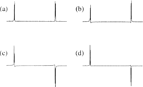
Figure 4: Experimental implementation of an algorithm to determine $f(0)$ on an NMR quantum computer. (a) The result of applying $U_{f_{00}}$; as this propagator is the identity matrix this spectrum can also serve as a reference. The lefthand pair of signals corresponds to the first spin ($I$), while the pair on the right hand side correspond to the second spin ($S$). Note that the signals from both spins (which are in state $|{0}\rangle$, the ground state) are in absorption. (b) The result of applying $U_{f_{01}}$; both sets of signals are still in absorption, as $f(0)=0$ for this function. (c) The result of applying $U_{f_{10}}$; the signals from spin $S$ are now in emission, since $f(0)=1$ for this function. (d) The result of applying $U_{f_{11}}$; the signals from spin $S$ are once again in emission as expected.

The lefthand pair of signals corresponds to the first spin ($I$), while the pair on the right hand side correspond to the second spin ($S$); the (barely visible) splitting in each pair arises from the scalar coupling $J_{IS}$. In this experiment the value of $f(0)$ is determined by setting both spins $I$ and $S$ into state $|{0}\rangle$, performing the calculation, and then measuring the final state of spin $S$; spin $I$ should not be affected, and so should remain in state $|{0}\rangle$. The phase of the reference spectrum (a) was adjusted so that signals from spin $I$ appear in absorption, and the same phase correction was applied to the other three spectra. The state of a spin after a calculation can then be determined by determining whether the corresponding signals in the spectrum are in absorption (state $|{0}\rangle$) or emission (state $|{1}\rangle$). As expected spin $I$ does indeed remain in state $|{0}\rangle$, while the value of $f(0)$ (determined from spin $S$) is $0$ for $U_{f_{00}}$ and $U_{f_{01}}$ but $1$ for $U_{f_{10}}$ and $U_{f_{11}}$.

Clearly our NMR quantum computer is capable of implementing this classical algorithm, as it is simple to determine $f(0)$. The other value, $f(1)$, can be determined in a very similar way (see figure 5).

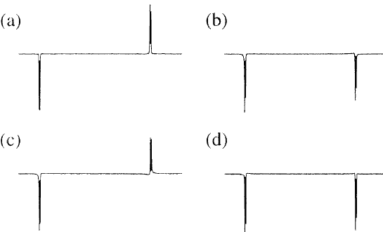
Figure 5: Experimental implementation of an algorithm to determine $f(1)$ on an NMR quantum computer; in this case the algorithm starts with spin $I$ in the excited state, $|{1}\rangle$, and so signals from spin $I$ are in emission. For details of the labelling see figure 4.

In this case spin $I$ remains in state $|{1}\rangle$, while $f(1)$ equals $0$ for $U_{f_{00}}$ and $U_{f_{10}}$ and equals $1$ for $U_{f_{01}}$ and $U_{f_{11}}$. There are, however, several imperfections visible in the results.

First, the signals are not perfectly phased: rather than exhibiting pure absorption or pure emission lineshapes the signals have more complex shapes, including dispersive components. These arise from the difficulty of implementing perfect selective pulses, which effect the desired rotation at one spin while leaving the other spin entirely unaffected. Similarly the selective pulses will not perfectly suppress J-couplings during the excitation, leading to the appearance of antiphase contributions to the lineshape. Any practical selective pulse will be imperfect, and so will result in systematic distortions in the final result. Note that these distortions are most severe in cases (b) and (c), where the propagator is complex, containing a large number of selective pulses. Interestingly the distortions are also more severe for the measurement of $f(0)$ (figure 4) than for $f(1)$ (figure 5); there is no simple explanation for this effect, which is due to the complex interplay of many selective pulses. We are currently seeking ways to minimise these effects.

Secondly, the signal intensities vary in different cases; as before the signal loss is most severe in cases (b) and (c), corresponding to complex propagators. This is in part a consequence of imperfect selective pulses, as discussed above, but may also indicate the effects of spin relaxation, that is decoherence of the states involved in the calculation. Decoherence is a fundamental problem, and may ultimately limit the size of practical quantum computers,[25, 26, 27] although a variety of error correction techniques[28, 29, 30] have been devised to overcome it.

These imperfections are not a major problem in our NMR quantum computer, as it is still easy to determine the state of a spin. However our computer is small, and the programs run on it are short (that is, they contain a small number of logic gates); if more complex programs are to be run on larger computers then these imperfections must be addressed.

The results of implementing the Deutsch quantum algorithm are shown in figure 6.

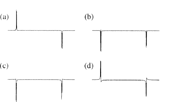
Figure 6: Experimental implementation of a quantum algorithm to determine $f(0)\oplus f(1)$ on an NMR quantum computer. In this case the result can be read out on spin $I$, that is using the signals on the left of the spectrum. For details of the labelling see figure 4. As expected the $I$ spin is inverted when the function is balanced ($f_{01}$ or $f_{10}$), but not when the function is constant ($f_{00}$ or $f_{11}$).

In this case the result ($f(0)\oplus f(1)$) can be read from the final state of spin $I$, while spin $S$ remains in state $|{1}\rangle$. As expected spin $I$ is in state $|{0}\rangle$ for the two constant functions ($f_{00}$ and $f_{11}$), but in state $|{1}\rangle$ for the two balanced functions ($f_{01}$ and $f_{10}$). Once again a number of imperfections are visible, though in this case they appear to be most severe in the case of $U_{f_{11}}$.

VI. SUMMARY

We have demonstrated that the isolated pair of ${}^{1}\rm H$ nuclei in partially deuterated cytosine can be used to implement a two qubit NMR quantum computer. This computer can be used to run both classical algorithms and quantum algorithms, such as that for solving Deutsch’s problem (distinguishing between constant and balanced functions). This is the first successful implementation of a quantum algorithm on any physical system[31].

This result confirms that NMR shows great promise as a technology for the implementation of small quantum computers. Difficulties do exist, largely as a result of the large number of selective pulses involved in the implementation of quantum gates, but we are currently seeking ways to overcome these problems. Even with the current level of errors it should be possible to build a three qubit computer capable of implementing more complex logic gates and algorithms.

References

- 1 R. P. Feynman, Int. J. Theor. Phys. 21, 467 (1982).
- 2 D. Deutsch, Proc. R. Soc. Lond. A 400, 97 (1985).
- 3 S. Lloyd, Science 273, 1073 (1996).
- 4 A. Ekert and R. Jozsa, Rev. Mod. Phys. 68, 733 (1996).
- 5 P. W. Shor, in Proceedings of the 35th Annual Symposium on the Foundations of Computer Science edited by S. Goldwasser (IEEE Computer Society, Los Alamitos, CA, 1994).
- 6 D. Deutsch, in Quantum Concepts in Space and Time edited by R. Penrose and C. J. Isham (Clarendon Press, Oxford, 1986).
- 7 D. Deutsch and R. Jozsa, Proc. R. Soc. Lond. A 439, 553 (1992).
- 8 R. Cleve, A. Ekert, C. Macchiavello, and M. Mosca, Proc. R. Soc. Lond. A 454, 339 (1998).
- 9 J. I. Cirac and P. Zoller, Phys. Rev. Lett. 74, 4091 (1995).
- 10 C. Monroe, D. M. Meekhof, B. E. KIng, W. M. Itano, and D. J. Wineland, Phys. Rev. Lett. 75, 4714 (1995).
- 11 D. G. Cory, A. F. Fahmy, and T. F. Havel, Proc. Natl. Acad. Sci. USA 94, 1634 (1997).
- 12 N. A. Gershenfeld and I. L. Chuang, Science 275, 350 (1997).
- 13 R. R. Ernst, G. Bodenhausen, and A. Wokaun, Principles of Nuclear Magnetic Resonance in One and Two Dimensions (Oxford University Press, Oxford, 1994).
- 14 See, for example, R. Laflamme, E. Knill, W. H. Zurek, P. Catasti, and S. V. S. Mariappan, NMR GHZ, available at the xxx.lanl.gov e-Print archive as quant-ph/9709025.
- 15 R. P. Feynman, Feynman Lectures on Computation edited by A. J. G. Hey and R. W. Allen (Addison-Wesley, Reading, MA, 1996).
- 16 C. H. Bennett, IBM J. Res. Develop. 17, 525 (1973).
- 17 A. Barenco. C. H. Bennett, R. Cleve, D. P. DiVincenzo, N. Margolus, P. Shor, T. Sleator, J. A. Smolin, and H. Weinfurter, Phys. Rev. A 52, 3457 (1995).
- 18 D. Deutsch, Proc. R. Soc. Lond. A 425, 73 (1989).
- 19 O. W. Sørensen, G. W. Eich, M. H. Levitt, G. Bodenhausen, and R. R. Ernst, Prog. NMR Spectrosc. 16, 163 (1983).
- 20 R. Freeman, Spin Choreography (Spektrum, Oxford, 1997).
- 21 R. Freeman, T. A. Frenkiel, and M. H. Levitt, J. Magn. Reson. 44, 409 (1981).
- 22 C. J. Bauer, R. Freeman, T. Frenkiel, J. Keeler, and A. J. Shaka, J. Magn. Reson. 58, 442 (1984).
- 23 H. Geen, X. Wu, P. Xu, J. Friedrich, and R. Freeman, J. Magn. Reson. 81, 646 (1989).
- 24 Ē. Kupc̆e and R. Freeman, J. Magn. Reson. A 105, 234 (1993).
- 25 I. L. Chuang, R. Laflamme, P. W. Shor, and W. H. Zurek, Science 270, 1633 (1995).
- 26 M.B. Plenio and P.L. Knight, Phys. Rev. A 53, 2986 (1996).
- 27 M. B. Plenio and P. L. Knight, Proc. R. Soc. Lond. A 453, 2017 (1997).
- 28 P. W. Shor, Phys. Rev. A 52, R2493 (1995).
- 29 A. Steane, Proc. R. Soc. Lond. A 452, 2551 (1996).
- 30 A. Steane, Phys. Rev. Lett. 78, 2252 (1997).
- 31 Since initial submission of this manuscript there has been considerable progress in this field, including another implementation of an algorithm to solve Deutsch’s problem[32], and two implementations of Grover’s quantum search algorithm[33, 34, 35].
- 32 I. L. Chuang, L. M. K. Vandersypen, X. Zhou, D. W. Leung, and S. Lloyd, Nature, in press.
- 33 I. L. Chuang, N. Gershenfeld, and M. Kubinec, Phys. Rev. Lett., in press.
- 34 J. A. Jones, M. Mosca, and R. H. Hansen, submitted to Nature.
- 35 J. A. Jones, Science, 280, 229 (1998).