Phase space caustics in multi-component systems

Abstract

As examples of quantum-“classical” coupling systems, multi-component systems are studied by semiclassical evaluations of the Feynman kernels in the coherent-state representation. From the observation of the phase space caustics due to the presence of the internal degree of freedom (IDF), two phenomena are explained in terms of the semiclassical theory: (1) The quantum oscillations of the IDF induce quantum interference patterns in the Hushimi representation; (2) Chaotic dynamics destroys the coherence of the quantum oscillations.

Coupling a quantum system with a “classical” system provides not only conceptual problems, e.g. the descriptions of measurement processes only in terms of unitary time evolutions [4], but also practical problems, e.g. interactions between electrons and nuclei in molecules [5, 6, 7]. The difficulty that the classical concept is inapplicable for the “classical subsystem” in the coupled system arises since the quantum and the classical subsystems become entangled [8] due to their interaction. However, it is possible to apply semiclassical methods, which elucidate quantum dynamics in terms of classical dynamics, to quantum-classical coupling systems. It is natural to treat only the classical subsystem with semiclassical methods for quantum-classical coupling systems, though it is formally simple to apply a semiclassical method to the whole system [7].

By applying a semiclassical theory only to the classical subsystem, this letter elucidates the following two phenomena of the quantum-classical coupling systems: The one is the interference phenomena of the classical subsystem due to the coupling to the quantum subsystem; The other is the destruction of the coherent quantum oscillation of the quantum subsystem by the “chaotic” dynamics of the classical subsystem. Note that the notion chaos in quantum dynamics can be introduced only through the semiclassical argument [9].

Throughout this letter, multi-component systems, e.g. electrons with a spin, and molecules that have quantized electrons, are employed as simple quantum-classical coupling systems. A quantum multi-component system consists of an internal and an “external” degrees of freedom (IDF and EDF, respectively): the IDF is a quantum subsystem, i.e. the IDF is conveniently described by matrices that have discrete indices rather than continuous indices; On the other hand, the EDF can be regarded as a “classical” system. Namely, it is natural to employ continuous-valued variables for describing the EDF.

Interference phenomena of a “classical” subsystem due to the coupling with a quantum system

The emergence of the quantum interference phenomena implies the complete breakdown of the classical picture. However, we can understand the interference phenomena with a semiclassical argument. In the following, I will study the interference phenomena produced by a time evolution in the Feynman kernel in the coherent state representation

$$K^{t}(q^{\prime\prime}p^{\prime\prime}\eta^{\prime\prime};q^{\prime}p^{\prime}\eta^{\prime})\equiv\left\langle q^{\prime\prime}p^{\prime\prime},\eta^{\prime\prime}\right|e^{-i\hat{H}t/\hbar}\left|q^{\prime}p^{\prime},\eta^{\prime}\right\rangle,$$ (1)

where $\hat{H}$ is a Hamiltonian, $\left|qp\right\rangle$ is an EDF’s coherent state [10], which is a natural correspondent of a point in the classical phase space, and $\left|\eta\right\rangle$ is an IDF’s state vector. Note that for the interference phenomena in $K^{t}$, or more generally, in the Hushimi representation of state vectors [11], we have an established semiclassical interpretation [12], which will be employed below.

In order to investigate the influence of IDF’s quantum oscillations on the EDF in a purified manner, the two-state linear curve crossing model for an infinitely heavy particle (for short, the heavy particle model) is studied. The IDF of this model is a two-level system, which is described by Pauli matrices. The heavy particle model is described by the Hamiltonian that does not have EDF’s kinetic term

$$\hat{H}\equiv\hat{V}(\hat{q})=-\hbar\hat{\sigma}_{z}F\hat{q}+\hbar\hat{\sigma}_{x}J.$$ (2)

The Hamiltonian is scaled by the Planck constant $\hbar$ in order to retain the independence of IDF’s time scales from $\hbar$. During a time evolution, the position of the EDF is an invariant. On the contrary, the momentum of the EDF is excited: In the absence of $J$, the EDF feel the force $+F$ ($-F$) when the state of the IDF is $\left|\uparrow\right\rangle$ ($\left|\downarrow\right\rangle$). The transition matrix element $J$ induces the quantum oscillation of the IDF between $\left|\uparrow\right\rangle$ and $\left|\downarrow\right\rangle$. Hence we lose the classical picture of the force acting on the EDF.

In order to treat only the EDF semiclassically, an effective action for the EDF is introduced:

$$S^{\rm eff}(q)=-i\hbar\ln Z(q),$$ (3)

where the “influence functional” [13] (cf. Ref. [14]) is defined as

$$Z(q)=\left\langle\eta^{\prime\prime}\right|{e^{-i\hat{V}(q)t/\hbar}}\left|\eta^{\prime}\right\rangle.$$ (4)

By employing $S^{\rm eff}$ as a “classical action”, the Feynman kernel $K^{t}$ is expressed as a coherent-state path integral [15] of the EDF. The semiclassical theory employed here is the stationary phase evaluation of the coherent-state path integral [16]. A stationary phase point is specified by the complex classical trajectory $(\bar{q},\bar{p})$ that obeys the following Hamilton equation (symplectic mapping)

$$\bar{p}^{\prime\prime}=\bar{p}^{\prime}+\partial S^{\rm eff}(\bar{q}^{\prime})/\partial q,\quad\bar{q}^{\prime\prime}=\bar{q}^{\prime},$$ (5)

where single- and double-primed quantities correspond to the initial and the final times, respectively. Furthermore, the “entrance label” $(q^{\prime},p^{\prime})$ and the “exit label” $(q^{\prime\prime},p^{\prime\prime})$ of $K^{t}$ specify the boundary condition of $(\bar{q},\bar{p})$ [16]

$$P^{\prime}=(p^{\prime}-iq^{\prime})/\sqrt{2},\quad Q^{\prime\prime}=(q^{\prime\prime}-ip^{\prime\prime})/\sqrt{2},$$ (6)

where $(Q,P)$ are defined by the linear canonical transformation $P=(\bar{p}-i\bar{q})/\sqrt{2}$ and $Q=(\bar{q}-i\bar{p})/\sqrt{2}$ [17]. A solution of (5) and (6) can be specified by the initial value of $Q^{\prime}$. The corresponding semiclassical amplitude is $E(Q^{\prime})\exp\{iF(Q^{\prime})/\hbar\}$, where $E$ and $F$ are the amplitude and the “action”, respectively. Klauder expected that the semiclassical Feynman kernel $K^{t}_{\rm SC}$ has always only single contribution of the semiclassical amplitude [16]. Actually, in a very short time scale, this is the case. However, Adachi showed that in general $K^{t}_{\rm SC}$ has multiple contributions of the semiclassical amplitudes in order to describe quantum interference phenomena [12].

In Fig. 1, the “exact” evaluation and the semiclassical evaluation of the Hushimi function $|K^{t}|^{2}$ are shown: the semiclassical theory reproduces the exact Hushimi function well. In the following, the semiclassical theory elucidates the structure of the Hushimi function. Since the initial condition of the IDF is $\left|\eta^{\prime}\right\rangle=\left|\uparrow\right\rangle$, the center of the amplitude of the EDF moves upward in the phase space due to the diagonal element $-\hbar Fq$ of Eq. (2). At the same time, there is a zero of the Hushimi function at $(q,p)\sim(0,-0.8)$. Namely, we encounter a quantum interference phenomenon.

In “single” component systems, quantum interference patterns in the Hushimi representation have intimate correspondence with phase space caustics (PSCs) [12], which are the zero points of the Jacobian $\partial Q^{\prime\prime}(Q^{\prime})/\partial Q^{\prime}$. At a PSC, the semiclassical amplitude $E=(\partial Q^{\prime\prime}/\partial Q^{\prime})^{(-1/2)}$ [18] diverges. Furthermore, around the PSC, a pair of semiclassical trajectories that are specified by two values of $Q^{\prime}$ appear for one value of the exit label $(q^{\prime\prime},p^{\prime\prime})$. The contributions of the resultant multiple semiclassical amplitudes to the Feynman kernel are controlled by the Stokes phenomena [19, 12]: In one region of the $Q^{\prime}$-plane, one of the semiclassical amplitudes is “unphysical” so must be excluded. The boundary of the unphysical region in the $Q^{\prime}$-plane is the Stokes lines; In the other region, the two semiclassical amplitudes contribute at once. Accordingly, a destructive interference pattern emerges in the Hushimi function [12]. Similarly as in the case of single component systems, a PSC produced the interference pattern in Fig. 1.

The dynamical origin of PSCs is the “folding” dynamics due to nonlinearity, especially the chaos, for the case of single component systems [12]. For multi-component systems, we encounter a brand-new source of PSCs, the logarithmic divergences of $S^{\rm eff}$ due to the zeros of the influence functional $Z$. Indeed the interference pattern in Fig. 1 (b) is due to such a PSC. The general feature around a zero point of $Z$ is explained by expanding $Z$ around the zero point [20, 21]. A zero of $Z$ produces a pair of PSC. One of the PSC can be safely ignored, since the value of $\Im F$ is too large to contribute to the Feynman kernel. For the other PSC, we must treat the Stokes phenomena. The Stokes lines in the $Q^{\prime}$-plane are shown in Fig. 2. According to the shape of these lines (looks like the upside-down “Venus” mark), I call the PSC that is caused by zeros of $Z$, v-PSC, in order to distinguish the conventional ones, which is called a-PSC, in the following argument.

The coherent quantum oscillation of the IDF produce the zeros of $Z$, as is explained below. With a given complex classical trajectory $\bar{q}$, the IDF is evolved by $\hat{V}(\bar{q})$. Hence, during a time evolution, the value of $Z$ oscillates due to the quantum oscillation of the IDF. In particular, $Z=0$ holds when the state vector of the IDF is orthogonal to $\left|\eta^{\prime\prime}\right\rangle$, which is specified by the exit label of $Z$. With a fixed value of $t$, we also encounter the zeros of $Z$ in varying $\bar{q}$.

The chaotic dynamics of the “classical” subsystem destroys the coherent quantum oscillation of the quantum subsystem

We saw above that the effect of IDF’s quantum oscillation appears as v-PSCs at EDF’s semiclassical dynamics. In turn, I will examine the effect of EDF’s dynamics, especially the chaotic dynamics, on v-PSCs by employing the spin-kicked rotor (the kicked rotor for a spin-$\frac{1}{2}$ particle) [22, 23]. The spin-kicked rotor is composed of a rotor as an EDF and a two-level system as an IDF and is described by the following Hamiltonian:

$$\hat{H}(t)\equiv T(\hat{p})\hat{1}_{\rm I}+\hat{V}(\hat{q})\sum_{n}\delta(t-n),$$ (7)

where $\hat{1}_{\rm I}$ is the identity operator of the IDF, $T(p)\equiv p^{2}/2$ and $\hat{V}(q)\equiv\hat{1}_{\rm I}K\cos q+\hbar\hat{\sigma}_{z}\delta K\cos q+\hbar\hat{\sigma}_{x}J$. This model is an extension of the standard mapping [24] to multi-component systems. Corresponding to the periodically time-dependent Hamiltonian $\hat{H}(t)$, we have a Floquet operator $\hat{U}=\exp[-iT(\hat{p})/\hbar]\exp[-i\hat{V}(\hat{q})/\hbar]$.

In Fig. 3, the time evolutions of the regular ($K=0.4$) and the chaotic ($K=2.4$) cases of quantities concerning to the IDF are shown. At the third step (indicated by arrows in the figures), the quantum oscillation continues in the regular case, but decays in the chaotic case. These different short time behaviors, which will be explained below by the semiclassical theory, determine the long-time behaviors of the system, i.e. the continuation of the coherent oscillation in the regular case (Fig. 3 (a)) and the destruction of the oscillation in the chaotic case (Fig. 3 (b)).

In order to give a semiclassical interpretation of the phenomena mentioned above, the “full” Feynman kernel $\left\langle q^{\prime\prime}p^{\prime\prime},\eta^{\prime\prime}\right|{\hat{U}^{N}}\left|q^{\prime}p^{\prime},\eta^{\prime}\right\rangle$ is studied by “decomposing” it by a sequence of the IDF’s states $\{\eta_{n}\}_{n=1}^{N-1}$

$$K^{N}_{\rm d}(q^{\prime\prime}p^{\prime\prime}\eta^{\prime\prime};\{\eta_{n}\}_{n=1}^{N-1};q^{\prime}p^{\prime}\eta^{\prime})$$ (8)

$$\equiv \left\langle q^{\prime\prime}p^{\prime\prime}\right|(\left\langle\eta_{N}\right|{\hat{U}}\left|\eta_{N-1}\right\rangle\ldots\left\langle\eta_{1}\right|{\hat{U}}\left|\eta_{0}\right\rangle)\left|q^{\prime}p^{\prime}\right\rangle,$$ (9)

where $\eta_{N}=\eta^{\prime\prime}$ and $\eta_{0}=\eta^{\prime}$. The decomposition of the kernel facilitate the semiclassical analysis: For the full kernel, we have to solve the EDF’s equation of motion that is nonlocal in time [6]; On the contrary, for $K^{N}_{\rm d}$, the equation of motion is local in time. In evaluating $K^{N}_{\rm d}$ by a stationary phase method concerning to the EDF, similar to the analysis of the heavy particle model (2), let us introduce an effective potential $V^{\rm eff}_{n}(q)\equiv i\hbar\ln Z_{n}(q)$, where $Z_{n}(q)\equiv\left\langle\eta_{n}\right|{\exp[-i\hat{V}(q)/\hbar]}\left|\eta_{n-1}\right\rangle$. The interaction term of the EDF’s effective action is $S^{\rm eff}_{\rm int}=-\sum_{n=1}^{N}V^{\rm eff}_{n}$. Accordingly, the classical equation of motion for the complex classical trajectory $\{(\bar{q}_{n},\bar{p}_{n})\}_{n}$ is

$$\bar{p}_{n}=\bar{p}_{n-1}-\partial V^{\rm eff}_{n}(\bar{q}_{n-1})/\partial q,\quad\bar{q}_{n}=\bar{q}_{n-1}+\bar{p}_{n}.$$ (10)

At the same time, Klauder’s boundary condition (6) is imposed on the complex classical trajectory.

In the semiclassical study of $K^{N}_{\rm d}$, v-PSCs appear with the similar mechanism mentioned above. Furthermore, we have to discuss the reconstruction of the full kernel from $K^{N}_{\rm d}$. However, concerning to the quantum oscillation of the IDF in the short time scale, the reconstruction of the full kernel plays no particular role, as is confirmed from the numerical observations. Hence, I report only the semiclassical study of $K^{N}_{\rm d}$.

In evaluating $K^{N}_{\rm d}$ semiclassically, a “physical” region $D$ on the $Q^{\prime}$-plane (i.e. iinitial points of the complex trajectory) is introduced [12]:

$$D=\{Q^{\prime}|\Im F(Q^{\prime})\leq(\Im F)_{\rm cutoff}\},$$ (11)

where $F$ is the classical action for $K^{N}_{\rm d}$. If $Q^{\prime}$ is out of the region $D$, the corresponding semiclassical amplitudes are too small to contribute to $K^{N}_{\rm d}$. Hence it is enough to count the contribution only from $D$ for the semiclassical Feynman kernel. For single component systems, a perturbation analysis shows that the chaotic dynamics makes $D$ contract exponentially fast around the classically realizable trajectory, whose stability exponent determines the rate of the contraction [21]. Although the multi-component systems do not have any classically realizable trajectory, the similar contraction of $D$ was observed in the numerical experiment in the chaotic case (Fig. 4 (b)). Furthermore, I observed that the contraction of $D$ have different influences on two kinds of PSCs; On one hand, a-PSCs produced by the chaotic dynamics catch up the contraction of $D$. Accordingly, a-PSCs have significant influence on the Feynman kernel, similarly to the single-component case; On the other hand, v-PSCs fail to catch up $D$ due to the contraction of $D$, though v-PSCs have strong influence in the regular case (Fig. 4 (a)). Due to the contraction of $D$, the unphysical region produced by v-PSCs become smaller. Furthermore, some v-PSCs move into the unphysical region produced by a-PSCs (Fig. 4 (b)). Consequently, contributions of v-PSCs, which implies the coherence of the IDF’s quantum oscillations, to the Feynman kernel is suppressed by the EDF’s chaotic dynamics and thus the IDF’s quantum oscillations, which have strong correspondence to the cause of v-PSCs, becomes incoherent (Fig. 3 (b)).

Discussion

The semiclassical method employed for the analysis of the spin-kicked rotor in the latter part of this paper has only a limited applicability: It is useful only for short time steps of quantum mapping systems and difficult to apply for quantum flow systems. Hence, we have to develop the semiclassical method that really works with the more general quantum-“classical” coupling systems. However, it is plausible that similar mechanisms obtained in this letter generally appear concerning to the interactions between the quantum oscillation of the quantum subsystem and the dynamics of the classical subsystem.

 

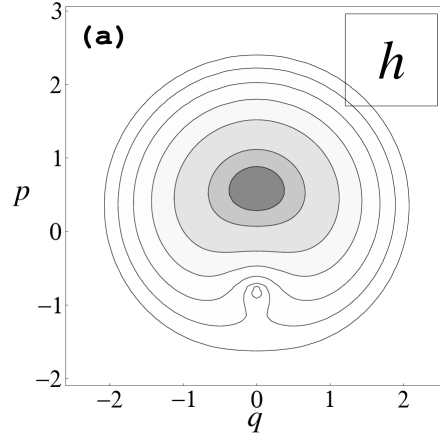
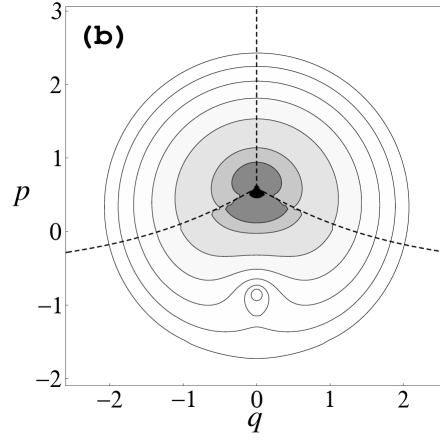
FIG. 1.: Contour plots of a Hushimi function $|K^{t}(qp\uparrow;q^{\prime}p^{\prime}\uparrow)|^{2}$ calculated by (a) the quantum theory and (b) the semiclassical theory. Parameters are $\hbar=h/(2\pi)=0.25$ (indicated by a box in (a)), $F=1.0$, $J=0.75$, $(q^{\prime},p^{\prime})=(0,0)$ and $t=1.5$. At the same time, the Stokes lines are indicated by dashed lines in (b).

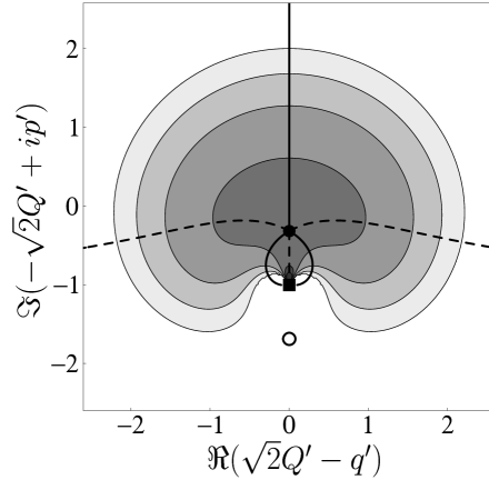
FIG. 2.: Contour plot of $\Im F(Q^{\prime})$, the imaginary part of the action for $K^{t}(q^{\prime\prime}p^{\prime\prime}\uparrow;q^{\prime}p^{\prime}\uparrow)$. The logarithmic divergent point of the effective action is indicated by $\blacksquare$. The corresponding pair of the PSC is indicated by $\bullet$ and $\circ$. As is explained in the main text, it is safe to ignore $\circ$. Accordingly, only for $\bullet$, the Stokes lines (bold), which are part of the pre-image of the Stokes lines in the $Q^{\prime\prime}$-plane, are drawn; Besides, the bold-dashed lines are the rest of the pre-image. The unphysical region is enclosed by the two Stokes lines that connect $\bullet$ and $\blacksquare$. Parameters are the same as in Fig. 1.

 

FIG. 3.: Time evolutions of $s_{z}\equiv\langle\hat{\sigma}_{z}\rangle$, $c\equiv\sqrt{\langle\hat{\sigma}_{x}\rangle^{2}+\langle\hat{\sigma}_{y}\rangle^{2}}$ and $P\equiv\sqrt{\langle\hat{\sigma}_{x}\rangle^{2}+\langle\hat{\sigma}_{y}\rangle^{2}+\langle\hat{\sigma}_{z}\rangle^{2}}$ [23] of (a) the regular case ($K=0.4$) and (b) the chaotic case ($K=2.4$). The initial condition is $\left|q^{\prime}p^{\prime},\uparrow\right\rangle$ with $(q^{\prime},p^{\prime})=(0.0,1.5)$. Parameters are $\hbar=0.25$, $\delta K=1.0$, and $J=0.75$. In the long time evolution, the oscillation of these quantities, especially $c$, are suppressed in the chaotic case (b).

 

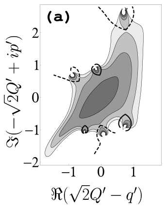
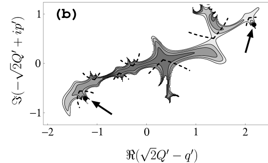
FIG. 4.: Contour plot of $\Im F(Q^{\prime})$ in the domain $D$ (11) ($(\Im F)_{\rm cutoff}=1.151$) of $K^{3}_{\rm d}(q^{\prime\prime}p^{\prime\prime}\uparrow;\{\uparrow,\uparrow\};q^{\prime}p^{\prime}\uparrow)$ for (a) the regular ($K=0.4$) and (b) the chaotic ($K=2.4$) cases. The Stokes lines that start from v-PSCs (solid lines) and a-PSCs (dashed lines) are also shown. Parameters are the same as in Fig. 3. In order to treat the Stokes phenomena, the region that are enclosed by the Stokes lines must be regarded as unphysical (non-contributing) region. Note that in the chaotic case (b), all of v-PSCs (indicated by $\bullet$ and pointed by arrows) in $D$ are in the unphysical region produced by a-PSCs.

- [1] Yukawa research fellow
- [2] E-mail: atanaka@cm.ph.tsukuba.ac.jp
- [3] Present address: Institute of Physics, University of Tsukuba, Tsukuba, Ibaraki 305-0006, Japan
- [4] See, e.g., B. d’Espagnat, Conceptual foundations of quantum mechanics (W. A. Benjamin, Massachusetts, 1976)
- [5] J. C. Tully and R. K. Preston, J. Chem. Phys. 55, 562 (1971); W. H. Miller and T. F. George, J. Chem. Phys. 56, 5637 (1972)
- [6] P. Pechukas, Phys. Rev. 181, 174 (1969); J. Cao, C. Minichino and G. A. Voth, J. Chem. Phys. 103, 1391 (1995)
- [7] G. Stock and M. Thoss, Phys. Rev. Lett. 78, 578 (1997)
- [8] E. Schrödinger, Proc. Camb. Phil. Soc. 31, 555 (1935)
- [9] M. C. Gutzwiller, Chaos in Classical and Quantum Mechanics (Springer-Verlag, New York, 1990)
- [10] J. R. Glauber, Phys. Rev. 131, 2766 (1963)
- [11] K. Hushimi, Proc. Phys. Math. Soc. Jpn. 22, 264 (1940); K. Takahashi and N. Saitô, Phys. Rev. Lett. 55, 645 (1985)
- [12] S. Adachi, Ann. Phys. 195, 45 (1989)
- [13] Since the time evolution under consideration can be regarded as a “unit time” evolution of a quantum mapping system, the Feynman path is a variable rather than a function of time.
- [14] R. P. Feynman and F. L. Vernon, Ann. Phys. 24, 118 (1963)
- [15] I. Daubechies and J. R. Klauder, J. Math. Phys. 26, 2239 (1985)
- [16] J. R. Klauder, in Path Integrals, Proceedings of the NATO Advanced Summer Institute, edited by G. J. Papadopoulos and J. T. Devreese, (Plenum, New York, 1978), p. 5; J. R. Klauder, in Random Media, edited by G. Papanicolauou, (Springer-Verlag, New York 1987), p. 163
- [17] P. Kramer, M. Moshinsky and T. H. Seligman, Group Theory and Its Applications III, 249 (1975)
- [18] A. Rubin and J. R. Klauder, Ann. Phys. 241, 212 (1995)
- [19] G. G. Stokes, Trans. Camb. Phil. Soc. 10, 106 (1864)
- [20] Around the zero of , we can regard as a prefactor of the oscillatory integral (i.e., exclude term from the effective action). However, such treatment prevent our understanding of the stationary points in a uniform manner in the -plane.
- [21] Atushi Tanaka, in preparation
- [22] R. Scharf, J. Phys. A: Math. Gen. 22, 4223 (1989)
- [23] A. Tanaka, J. Phys. A: Math. Gen. 29, 5475 (1996)
- [24] B. V. Chirikov, Phys. Rep. 52, 263 (1979); G. Casati et al., Lecture Notes in Physics 93, 334 (1979)