Quantised motion of an atom in a Gaussian-Laguerre beam

Abstract

We quantise the centre of mass motion of a neutral Cs atom in the presence of a classical Gaussian-Laguerre₁₀ light field in the large detuning limit. This light field possesses orbital angular momentum which is transferred to the atom via spontaneous emissions. We use quantum trajectory and analytic methods to solve the master equation for the 2d centre of mass motion with recoil near the centre of the beam. For appropriate parameters, we observe heating in both the cartesian and polar observables within a few orbits of the atom in the beam. The angular momentum, $\hat{L}$, shows a rapid diffusion which results in $\langle\hat{L}\rangle$ reaching a maximum and then decreasing to zero. We compare this with analytic results obtained for an atom illuminated by a superposition of Gaussian-Laguerre modes which possess no angular momentum, in the limit of no recoil.

03.75.Be

I Introduction

Recently there has been a growing interest, both in theory and experiment, in the interaction between matter and light fields possessing orbital angular momentum [1]. The typical light fields used in these works are the Gaussian-Laguerre modes (G-L). Experimental work has concentrated on two areas; the study of the motion of microscopic particles in Gaussian-Laguerre beams [2], and the use of such beams in atom trapping [3]. The theoretical work so far has solely concentrated on the semi-classical description of the motion of matter in G-L beams [4]. As neutral atom cooling improves, a truly quantum description becomes necessary. Indeed, recent experiments in atomic guiding using evanescent waves within a hollow optical fibre verge on the quantum regime [5]. In this paper we examine the quantised motion of a neutral atom in a Gaussian-Laguerre₁₀ mode, taking into account the spontaneous recoil while in the far detuned limit. We are primarily interested in the quantised transfer of the orbital angular momentum to the centre-of-mass (COM) of the atom and how this appears in the quantal evolution. In the limit where the incident light is far detuned from the atom’s natural frequency, we find that the transfer of angular momentum is imparted through the dissipation suffered by the atom through spontaneous recoil. We derive a master equation for the COM motion in the limit of large detuning for motion near the centre of the beam which includes the momentum kick from spontaneous recoil. We select the beam and atomic parameters which give an atom that can be easily cooled to the lowest COM eigenstate of the G-L beam and which suffers a large amount of spontaneous recoil. This results in a rapid increase of angular momentum over the orbital time of the atom around the center of the beam. The atom, because of the dissipation caused by the spontaneous recoil, also heats up. This is indicated by an increase in the variances of $x$ and $p$.

For the case of a neutral Cesium atom, we solve the master equation using quantum trajectories and numerically compute expectation values and variances for the atom’s orbital angular momentum, cartesian position and momentum. We solve for an atom initially in a minimum uncertainty state (1) at the centre of the beam and, (2) offset from the centre. We find that the variances increase with time as the system heats due to the diffusion caused by the spontaneous recoil. Surprisingly, we also find both in (1) and (2), that the diffusion in the angular momentum $\hat{L}$, is so rapid that $\langle\hat{L}\rangle$ reaches a maximum and then decreases to zero. This is to be contrasted with the semiclassical work [4], which shows a general increase in the atom’s semiclassical angular momentum while in the harmonic regime of the light field potential. We finally compare this system to a similar master equation with no cross terms and no momenta transfer on recoil. This corresponds to an atom coupled to a superposition of G-L₊₁₀ and G-L_-10 modes in the semiclassical limit. Here no angular momentum is transferred but the variances in both $x$ and $y$ remain much smaller than in the case where recoil is included.

II Gaussian-Laguerre Modes and Master Equation

Gaussian Laguerre modes can be produced through cylindrical lens mode converters [7], spiral phase plates [6] and through computer generated holograms [8]. The general form for the electric field for the Gauss-Laguerre_l0 mode is [8]

$$E_{l0}^{+}=E_{0}\left(\frac{r}{w}\right)^{l}e^{-(r/w)^{2}}e^{\pm il\theta}e^{-i\frac{kr^{2}}{2R}}e^{i(kz+\Phi)}$$ (1)

where $w$ is the beam waist, $R$ is the wavefront radius of curvature and $\Phi$ is the Guoy phase shift. For most applications the paraxial approximation is quite good. In this approximation it has been shown [9, 10] that the Guoy phase and Rayleigh curvature are very small for Gaussian-Laguerre modes near the beam waist and we shall ignore them. We thus restrict the atom’s motion to a two dimensional plane transverse to the beam propagation direction, positioned at the beam waist. We shall concentrate on the $l=+1$ mode. Near the centre of the beam the exponential dependence on $r$ is small and we shall also ignore it.

When the system is near resonance the internal electron degrees of freedom are strongly coupled to the external spatial degrees of freedom of the atom. To solve this fully quantum mechanically, for two spatial degrees of freedom, is virtaully impossible. To simplify matters, we work in the far detuned regime. In this regime, the master equation, in the dipole approximation, and adiabatically eliminating the dynamics of the internal excited state (assuming a two-level atom), takes the form [11]

$$\frac{d}{dt}\rho = -\frac{i}{\hbar}\left[\frac{1}{2m}(p_{x}^{2}+p_{y}^{2})+\frac{\hbar|\hat{\Omega}|^{2}}{\Delta|\nu|^{2}},\,\rho\right]$$ (2)

$$+ \frac{\Gamma}{2\Delta^{2}|\nu|^{2}}\left(2{\cal N}\hat{\Omega}\rho\hat{\Omega}^{\dagger}-\left\{\hat{\Omega}^{\dagger}\hat{\Omega},\,\rho\right\}\right)\;\;,$$ (3)

where $\hat{\Omega}$ is the spatially dependent Rabi frequency, $\Delta$ is the detuning, and $|\nu|^{2}=1+\Gamma^{2}/(2\Delta^{2})$. The super operator ${\cal N}$, describes the effect of a spontaneous emission on the atom [12],

$${\cal N}\rho=\int\,d\vec{n}\,\Phi(\vec{n})\,e^{ik\vec{n}\cdot\vec{x}}\rho e^{-ik\vec{n}\cdot\vec{x}}\;\;,$$ (4)

where $\Phi(\vec{n})$ is the dipole emission probability function which is defined to be [13]

$$\Phi(\vec{n})=\frac{3}{8\pi}\left(1-\frac{(\vec{d}\cdot\vec{n})^{2}}{\vec{d}\cdot\vec{d}}\right)\;\;,$$ (5)

for plane-polarised incident light and

$$\Phi(\vec{n})=\frac{3}{16\pi}\left(1+(\vec{z}\cdot\vec{n})^{2}\right)\;\;,$$ (6)

for circularly polarised incident light. Here $\vec{n}$ is the unit vector giving the direction of the spontaneously emitted photon, $\vec{d}$ is the direction of the atomic dipole, and $\vec{z}$ is along the direction of beam propagation.

Before continuing we will discuss the validity of the two assumptions made above. From considerations that will follow, we will choose to work with the $P_{3/2}\rightarrow S_{1/2}$ transition in Cs. Firstly, to consider this to be a two-level atom we must excite the $P_{+3/2}\leftrightarrow S_{+1/2}$ or $P_{-3/2}\leftrightarrow S_{-1/2}$ transitions. This can be done with incident $\sigma_{\pm}$ circularly polarised light. Plane polarised incident light does not result in a closed 2-level atomic system. Thus, we must take (6) as the angular probability distribution for the direction of spontaneous emission of photons.

Secondly, we have chosen to work in the dipole approximation. We now explain why this approximation is still valid even though the COM is quite cold. The electronic transitions occur on much faster timescales than the dynamics of the COM. Thus, although the COM is cooled to where the de-Broglie wavelength of the COM degree of freedom is relatively large, the electronic degrees of freedom with which the atom and light interact are not cooled and can rapidly follow the slow COM motion. Thus the electric dipole approximation holds when the spatial gradients of $|\Omega|^{2}$ are small on the scale of the electronic clouds involved in the transition and not on the scale of the de-Broglie wavelength of the COM. To obtain field gradients large enough to significantly excite higher multipoles one must be working in the extreme non-paraxial regime. The degree to which the Gauss-Laguerre modes are non-paraxial and thus couple to higher multipoles is extremely small. For the physical model discussed in this paper we can estimate the ratio of the azimuthal spin-orbit force to the transverse electric field force to be $F_{s-1}/F_{\phi}\sim 6\times 10^{-6}$, [14]. The omission of higher multipoles is therefore a very good approximation for these modes. One consequence of this approximation is that the exchange of spin angular momentum is conserved separately from the exchange of orbital angular momentum [15], i.e. there is very little spin-orbital coupling. Since $\Phi(\vec{n})$ is insensitive to the sign of the helicity of the incident light and the Clebsch-Gordan coefficients for the transitions in Cs are symmetric under $\sigma\rightarrow-\sigma$ we are forced to conclude that the quantum evolution of the COM is highly insensitive to the helicity of the incident light. This conclusion, although quite reasonable on the atomic scale, seems to be at odds with recent experiments on the “classical” motion of micro-spheres illuminated by circularly polarised Gaussian-Laguerre beams [2, 1]. There are two possible physical mechanisms which could generate the observed rotation in mesoscopic particles. The transfer of spin angular momentum to orbital angular momentum could be mediated through some bifrefringence present in the material, akin to Beth’s original experiment. However, the transfer could also be mediated through non-radiative off-resonant couplings, i.e. absorption. Although the first mechanism might play some small part in the experiments, recent results seem to indicate that absorption is the primary mechanism which couples both the spin and orbital angular momentum of the light, to the orbital angular momentum of the mesoscopic particles [17, 2]. However, in the quantum system studied here, the spin-orbit coupling, as we have argued above, for a single atom interacting with a Gaussian-Laguerre beam should be quite small. An experiment to probe the dependence of the COM motion of ultra-cold atoms on the incident light’s helicity would be quite illuminating.

A Master Equation

We begin by recasting the master equation (3) into a more convenient form. We first set $\hat{\Omega}=(\Omega_{0}/w)\,\tilde{\Omega}$ where $\tilde{\Omega}=\hat{r}\exp\,(i\hat{\theta})=\hat{x}+i\hat{y}$. Next, we obtain the orbital frequency of the atom in the GL₁₀ mode in the harmonic approximation to be

$$\omega_{s}^{2}=\frac{2\hbar\Omega_{0}^{2}}{m\Delta|\nu|^{2}w^{2}}\;\;,$$ (7)

where $m$ is the mass of the atom. We further include the following rescalings to give a master equation with coefficients of order unity in the dimensionless quantities, $\bar{X},\bar{Y},\bar{P}_{\bar{x}}$, and $\bar{P}_{\bar{y}}$,

$$\hat{x}=\alpha_{x}\bar{X}\;\;,\;\; \hat{p}_{x}=\alpha_{p}\bar{P}_{\bar{x}}\;\;,$$ (8)

$$\hat{y}=\alpha_{x}\bar{Y}\;\;,\;\; \hat{p}_{y}=\alpha_{p}\bar{P}_{\bar{y}}\;\;,$$ (9)

$$\alpha_{x}=\frac{1}{\sqrt{\beta}}\sqrt{\frac{\hbar}{m\omega_{s}}\;\;,\;\;} \alpha_{p}=\frac{1}{\sqrt{\beta}}\sqrt{\hbar m\omega_{s}}\;\;,$$ (10)

with $\tau=\omega_{s}t$. This gives $[\bar{X},\bar{P}_{\bar{X}}]=i\beta$, where $\beta$ serves as the rescaled Planck’s constant. Letting $\eta=\Gamma/(4\Delta\beta)$, we finally obtain

$$\frac{d}{d\tau}\rho = -\frac{i}{2\beta}\left[\bar{P}_{\bar{x}}^{2}+\bar{P}_{\bar{y}}^{2}+\bar{X}^{2}+\bar{Y}^{2},\,\rho\right]$$ (11)

$$- \eta\left(2{\cal N}(\bar{X}+i\bar{Y})\rho(\bar{X}-i\bar{Y})-\left\{\bar{X}^{2}+\bar{Y}^{2},\,\rho\right\}\right)\;\;.$$ (12)

For an atom cooled to the recoil limit, $P_{recoil}=\hbar k$ or

$$\bar{P}_{r}=\sqrt{\beta}\sqrt{\frac{\hbar k^{2}}{m\omega_{s}}}\;\;.$$ (13)

If the atom is initially in a pure, minimum uncertainty state, we have

$$\Delta\bar{P}_{r}=\sqrt{\beta}\sqrt{\frac{\hbar k^{2}}{m\omega_{s}}}\;\;,\;\;\Delta\bar{X}_{r}=\frac{\beta}{2\Delta\bar{P}_{r}}\;\;,$$ (14)

while the effect of the exponential in the superoperator ${\cal N}$ is to shift the momentum,

$$e^{-ik\alpha_{x}\bar{X}}\,\bar{P}_{\bar{X}}\,e^{+ik\alpha_{x}\bar{X}}=\bar{P}_{\bar{X}}+\mu\beta\;\;,$$ (15)

where $\mu=k\alpha_{x}$. We note that the master equation (12) is more involved than the majority of master equations previously discussed within the literature. The complications here are twofold. In the Linblad form for the master equation (12), the output channel is not just a momentum jump (as it is in the near-resonance situation) but is a combination of a diffusion in space and momenta. Secondly, we note the presence of cross terms between $\bar{X}$ and $\bar{Y}$ in the dissipation. This cross-coupling frustrates the derivation of any simple equation or set of equations for the time evolution of ensemble averages. Finally, if $\mu\beta$ is much smaller than the momentum variance of the wavepacket $\langle\Delta\bar{P}\rangle$, then the exponential operator in (15) can be expanded to first order in $\bar{X}$. One can then explicitly perform the stochastic average over $d\vec{n}$ to arrive at a Linblad type master equation. This can be converted into a c-number Fokker-Planck equation which (since it is at most quadratic), will give, in the large energy regime, expectation values which agree with the semi-classical theory. However, below we will choose the system parameters such that $\mu\beta$ is large and thus one must solve the full quantum dynamics of (12).

B Quantum Trajectories

The master equation (12) must be solved numerically. We will use the method of Quantum Trajectories [18]. However, we will be able to solve for the non-unitary evolution analytically between jumps. This is possible only in the harmonic approximation for motion near the centre of the beam. To use this technique we rewrite the master equation (12) in the form

$$\frac{d}{d\tau}\rho = -\frac{i}{\beta}\left[H_{0},\rho\right]$$ (16)

$$+ \int\,d^{2}\vec{n}\,\left[2C(\vec{n})\rho C^{\dagger}(\vec{n})-\left\{C^{\dagger}(\vec{n})C(\vec{n}),\rho\right\}\right]\;\;,$$ (17)

where

$$C(\vec{n}) \equiv \sqrt{\eta\Phi(\vec{n})}(\bar{X}+i\bar{Y})\,e^{i\mu(\epsilon_{x}\bar{X}+\epsilon_{y}\bar{Y})}\;\;,$$ (18)

$$2H_{0} \equiv \bar{P}_{\bar{X}}^{2}+\bar{P}_{\bar{Y}}^{2}+\bar{X}^{2}+\bar{Y}^{2}\;\;,$$ (19)

and where $\epsilon_{x,y}$ are the $x$ and $y$ components of the recoil direction vector $\vec{n}$. To apply the method we first choose an initial state $\rho_{0}=\sum_{i}|\Psi_{i}\rangle\langle\Psi_{i}|$. In our case we will set the initial state to be a pure coherent state. From the ensemble $\rho_{0}$ we choose a particular $|\Psi_{i}\rangle$ at random and apply the following procedure. We generate a uniform random variable $\zeta\in[0,1]$, and evolve the pure state $|\Psi_{i}\rangle$ using the non-unitary Hamiltonian $H_{non}$,

$$H_{non}\equiv H_{0}-i\beta\int\,d^{2}\vec{n}\,C^{\dagger}(\vec{n})C(\vec{n})=H_{0}-\delta(\bar{X}^{2}+\bar{Y}^{2})\;\;,$$ (20)

where $\delta=i\beta\eta$. We evolve for a time $\tau_{\zeta}$ such that, $|\langle\Psi(\tau_{\zeta})|\Psi(\tau_{\zeta})\rangle|^{2}=\zeta$. We then apply the “Jump” operator $C(\vec{n})$, to $|\Psi(\tau_{\zeta})\rangle$, $C|\Psi\rangle\rightarrow|\Psi^{\prime}\rangle$, where the vector $\vec{n}$ is generated by two random numbers taken from the distribution $\Phi(\vec{z},\vec{n})$, (6). We then renormalise the state $|\Psi^{\prime}\rangle$ and repeat the procedure beginning with the generation of a new uniform random waiting time, $\zeta$. At set intervals $\tau_{s}$, we store the state. Repeating this whole procedure, starting with randomly sampled $|\Psi_{i}\rangle$ from the ensemble $\rho_{0}$, we generate estimates for the density matrices at the times $\tau_{s}$. From these estimates we can calculate expectations and variances for various observables. In practice, unless the final quantities involve the computation of off-diagonal elements of the $\rho(\tau_{s})$, one only needs to store the incremental values for these quantities and not the complete $\rho(\tau_{s})$ themselves. This produces enormous savings on hard memory usage since the storage size of a single state $|\Psi_{i}\rangle,$ in a truncated Fock state basis of 40, in two dimensions, is approximately 25KB in double precision.

As stated above, in the harmonic approximation, $H_{non}$ is quadratic and the propagator, $U_{non}=\exp\,(iH_{non}\tau)$, can be evaluated analytically in the Fock state basis. This basis is constructed through the operators

$$a_{\bar{X}}^{\dagger}=(\bar{X}-i\bar{P}_{\bar{X}})/\sqrt{2\beta}\;\;,\;\;a_{\bar{Y}}=(\bar{X}+i\bar{P}_{\bar{X}})/\sqrt{2\beta}\;\;,$$ (21)

for the $x$ and similarly for the $y$ direction. From these definitions we can easily see that $[a_{x},a_{x}^{\dagger}]=1$. In terms of these operators the non-unitary Hamiltonian takes the form

$$H_{non} = \beta\left[(1-\delta)(a_{\bar{X}}^{\dagger}a_{\bar{X}}+a_{\bar{Y}}^{\dagger}a_{\bar{Y}})\right.$$ (22)

$$- \left.\frac{\delta}{2}(a_{\bar{X}}^{\dagger 2}+a_{\bar{X}}^{2}+a_{\bar{Y}}^{\dagger 2}+a_{\bar{Y}}^{2})+(1-\delta)\right]\;\;,$$ (23)

Analytically evaluating the propagator $U_{non}(\tau)$ is quite tedious and is left to Appendix 1. Inverting, $|\langle\Psi_{i}|U_{non}^{\dagger}(\tau_{\zeta})U_{non}(\tau_{\zeta})|\Psi_{i}\rangle|^{2}=\zeta$, to obtain $\tau_{\zeta}$ is not possible analytically and was performed numerically using Brent’s algorithm [19].

To compute the effect of the Jump operator $C(\vec{n})$ on the state in the Fock basis is quite involved. A number of schemes have been used previously to increase the efficiency of the quantum trajectory method in the case where the quantum jump is a pure momentum kick [20, 21]. These schemes will not work in this case as the jump operator, (18), is not a pure momentum kick. One could perform this jump sequentially by applying the momentum shift in the $\bar{P}$ basis, fast Fourier transforming (FFT) into the $\bar{X}$ basis, and then applying $\bar{X}^{2}$. Since we are capable of computing the jump analytically we doubt that the FFT method would prove more efficient in this case. In the more realistic (and more complicated) case where we do not make the harmonic approximation, no analytical results seem to be possible and the FFT method would be necessary. The computation of the effect of the Jump operator on the state is given in Appendix 2.

Finally, the generation of the random direction $\vec{n}$, for the recoil of the atom from the distribution (6) is explained in Appendix 3.

C Atomic Parameters

In this section we set out the ingredients necessary for a quantum description of the evolution of the COM. We require an atom which can be easily cooled to significantly populate the lowest vibrational levels of the G-L mode. The dissipation must be large enough to observe decay of the system within the timescale of the orbital period of the atom around the mode. If the dissipation is too weak then the dynamics are washed out and a secular approximation, averaging over a cycle time, would be a good description of the evolution. This condition can be roughly approximated by setting the recoil frequency equal to the orbital frequency of the harmonic well, $\omega_{s}=\hbar k^{2}/2m$.

These two conditions coupled with that of the large detuning are quite difficult to achieve. For most atoms, the “hole” in the beam is very dark and the dissipation coefficient $\eta$, is very small. This makes such a mode quite good for trapping the atom in a region of low dissipation [3]. To achieve high dissipation $\eta$, we must make $\Gamma/\Delta$ as large as possible. To enforce the large detuning limit we must also have $\Delta>\Gamma$, $\Delta>\Omega_{0}$. All of these conditions imply $\Omega_{0}\sim\Gamma\sim\Delta$. For atoms with very low Doppler temperatures (Calcium), these conditions are hard to meet as usually $\Gamma\ll\Omega_{0}$ (for modest beam intensities). Instead we choose to look at Cesium, cooled to recoil. For the Cs atom, with $m=0\cdot$665$\times 10^{-25}$kg, $\lambda=657$nm, $\Gamma/2\pi=5\cdot 3$MHz, with a Gaussian-Laguerre beam of intensity $I=4$W/m², and width $w=2\times 10^{-5}$m, we get a Rabi frequency $\Omega_{0}/2\pi\approx 5$MHz. Choosing $\Delta\sim 3\Gamma$ or $\Delta/2\pi\sim 16\cdot 4$MHz we obtain an orbital frequency of $\omega_{s}/2\pi\sim 774$Hz. The ratio $E_{recoil}/E_{ground}\sim 2\cdot 6$, indicates a high population in the ground vibrational state of the well. Choosing $\beta=0\cdot 25$, we have $\alpha_{x}=0\cdot 6\mu$m, $\alpha_{p}=0\cdot 6\times 10^{-27}$m/s, $\eta=0.0125$ and $\mu=2.310$. For an atom cooled to recoil in a pure minimum uncertainty state (14) we get $\Delta\bar{P}_{r}\sim 0\cdot 58$, and $\Delta\bar{X}_{r}\sim 0\cdot 22$. Since the momentum shift from the bare recoil kick is, $\bar{P}\rightarrow\bar{P}+0\cdot 57$, and is thus on the same scale as the quantum wavepacket we must use the full quantal master equation to describe the evolution. For simplicity, we set the initial wavepacket to be a minimum uncertainty state with equal variances in both $\bar{P}$ and $\bar{X}$ so that $\Delta\bar{X}=0\cdot 35$. In the rescaled time $\tau$ the period is $2\pi/\beta=8\pi\approx 25$.

D Numerical Simulation

We first simulate the dynamics of the atom initially positioned at the centre of the trap. We plot only the mean and variance for the cartesian position, momentum and polar angular momentum of the atom. The angular momentum operator is given in the position representation as $\hat{L}\equiv(\bar{X}\bar{P}_{\bar{Y}}-\bar{P}_{\bar{X}}\bar{Y})$. In the Fock basis this becomes $\hat{L}=i\beta(a_{\bar{X}}a_{\bar{Y}}^{\dagger}-a_{\bar{X}}^{\dagger}a_{\bar{Y}})/2$. The code was run on two Sun Hyper-Sparcs and took approximately 100 CPU hours to produce $\sim$ 300 trajectories. The results of this simulation are shown in Figure 1. From the cylindrical symmetry we should have $\langle\bar{X}\rangle=0$ and $\langle\bar{P}_{\bar{X}}\rangle=0$. This is well approximated in the data as seen in Fig. 1a. In Fig. 1b the variances in both $\bar{X}$ and $\bar{Y}$ increase with time as the dissipation heats the system. We notice a slight tailing off of this heating near $\tau=80$. We cannot be entirely sure that this is not due to truncation effects as the wavepacket spreads out to regions of large laser intensity and undergoes frequent recoil. The plots of $\langle\bar{X}\rangle$ and $\langle\bar{Y}\rangle$ still remain close to zero and one might suspect that this decrease in heating rate may be a real effect. A more surprising result can be seen in Fig. 1c. Here, we see an initial increase in $\langle\hat{L}\rangle$ and $\langle\hat{L}^{2}\rangle$. The variance is at all times larger than the average. The average reaches a maximum and then decreases towards zero as $\tau$ increases beyond $\tau=50$. This is not a truncation error and is due to the very rapid increase in variance after $\tau=50$. The diffusion of $\hat{L}$ becomes so fast that the average quickly drops to zero.

In the second simulation the atom is initially again in a minimum uncertainty state but with an initial position $\bar{X}=1,\;\bar{Y}=0$, and initial momentum $\bar{P}_{\bar{X}}=0,\;\bar{P}_{\bar{Y}}=1$. In the absence of dissipation the atom will rotate in the $\bar{X}-\bar{Y}$ plane about the origin with a period of $\tau_{p}=2\pi/\beta=8\pi\sim 25$. This second simulation took longer to run since there were many more jumps per trajectory ( to $\tau=80$ ) than in the first simulation. The reason for this is that the initial wavepacket is in a region of higher laser intensity and thus undergoes more frequent spontaneous emissions. Computing times grew too lengthy on the Hyper-Sparcs. It became necessary to parallelise the code which was then run on a multiprocessor SGI Power Challenger. The results shown below consist of approximately 300 trajectories and correspond to 50 CPU hours on the Power Challenger. The results of the second simulation are shown in Figure 2. We see essentially the same overall behavior as in the first simulation. Heating is shown by the increase in the variances of $\bar{X}$ and $\bar{Y}$ (Fig. 2b). The variance in $\hat{L}$ again increases faster than the mean and $\langle\hat{L}\rangle$, after gaining a maximum, falls to zero again (Fig. 2c). In Figure 3 we have plotted the $\bar{X}-\bar{Y}$ probability distribution of the estimated $\rho$ at various times in the evolution. To gauge the truncation errors we have plotted in Fig. 4a a histogram of the number of jumps occurring within a given time interval as a function of time. From this and the squarish probability profile in the $\bar{X}-\bar{Y}$ plane we see that truncation effects become significant after $\tau=40$.

In Appendix D we solve the master equation (12), without the exponential recoil kick and coupled cross terms in the dissipation. This corresponds to semi-classical evolution (the momentum shift becoming negligible with respect to the size of the wavepacket) of the atom illuminated by a coherent superposition of G-L₊₁₀ and G-L_-10 modes. We see that in this case $\langle\Delta\bar{X}\rangle$ increases without bound but remains below the values obtained in the numerical simulations. This is to be expected as there is no recoil here. This result gives us a rough analytical check on the numerics of the simulation.

III Conclusion

In this work we have studied the quantum dynamics of the two dimensional spatial COM motion of an ultra-cold Cesium atom cooled to recoil moving near the center of a Gaussian-Laguerre₁₀ light field in the far detuned regime. We found that the transfer of orbital angular momentum from the light field to the atom is mediated by spontaneous emissions. In the appropriate limit we find that the orbital motion of the atom is not very sensitive to the helicity of the illuminating light field. We argue that the helicity dependence seen in mesoscopic experiments may be due to residual birefringence present in the material. For motion near the center of the beam we made an harmonic approximation to the light potential. In this approximation we solved the quantum dynamical master equation using the quantum trajectories method. With the harmonic approximation we were able to solve for the non-unitary and jump evolutions analytically. This significantly increased the computational efficiency of the numerics. Two seperate initial conditions were used. In the semiclassical regime, in the harmonic approximation and with the same initial conditions, the atom gains a net angular momentum. In the quantum regime, for the particular physical parameters chosen, we found that the diffusion of the angular momentum was very high with the result that $\langle\hat{L}\rangle$ reached a maximum at a time $\tau_{c}$, and then decreased to zero. As an analytical check we solved for the quantum evolution of the atom illuminated by a superposition of G-L₊₁₀ and G-L_-10 light in the limit of no recoil. The variances found were smaller than those seen in the fully quantum computation as expected. From similiar studies in other systems one might expect that $\tau_{c}$ will increase with an increase in the initial state energy or a decrease in the dissipation rate. However, to explore the parameter space of this system more fully and include the complete exponential character of the light field potential would require a very significant increase in computational resources. With the inclusion of the exponential in the potential and dissipation terms of the master equation we would expect to see shear in the evolution of the wavepacket. Partial revivals and cat states might be expected as these have been seen in other nonlinear potentials. We note that unless some new analytical techniques are found further investigations into this system will be very computationally expensive.

Finally, experimental probing of $\langle\hat{L}\rangle$, for ultra-cold atoms in the center of a Gaussian-Laguerre trap could be attempted using the azimuthal Doppler shift provided by the rotation of the atoms about the axis of the beam [25]. One might double the shift by retro-reflecting the laser probe beam back through the rotating atomic cloud while maintaining the reflected beam’s impact parameter to the axis to be the same as the incident beam’s impact parameter. In order to achieve a good Doppler signal it may be necessary to work in a regime where the orbital frequency of the atomic cloud near the center of the G-L mode is higher than that used in this work.

Acknolwedgements

We thank S. Dyrting, G. Milburn, H. Wiseman, J. Steinbach and D. Segal for helpful comments on this work. This work was made possible through a Human Capital and Mobility Fellowship from the European Union.

A Matrix elements for $U_{non}$

In this appendix we calculate the matrix elements of the non-unitary propagator $U_{non}$ in the number state basis. Although the following calculations are somewhat involved the resulting analytic expression proved more efficient than a direct numerical integration of the equations. We begin with the general Fock state basis matrix element

$$\langle m_{x},m_{y}|e^{-iH_{non}\tau/\beta}|n_{x},n_{y}\rangle=$$ (A1)

$$e^{-i\tau(1-\delta)}\langle m_{x}|\exp\left\{-i\tau\left[(1-\delta)a_{x}^{\dagger}a_{x}-\frac{\delta}{2}(a_{x}^{\dagger 2}+a_{x}^{2})\right]\right\}|n_{x}\rangle$$ (A2)

$$\times\langle m_{y}|\exp\left\{-i\tau\left[(1-\delta)a_{y}^{\dagger}a_{y}-\frac{\delta}{2}(a_{y}^{\dagger 2}+a_{y}^{2})\right]\right\}|n_{y}\rangle$$ (A3)

where $\delta=i\beta\eta$.

To evaluate this we use Baker-Campbell-Hausdorff (BCH) disentangling. The particular methods is due to Wilkox [22]. For simplicity we take first the $x$ matrix elements and drop the $x$ subscript. We then write $U_{non}=\exp\,({\cal H})$ where ${\cal H}\equiv xK_{0}+y(K_{+}+K_{-})$, and where $K_{0},K_{\pm}$ are the generators of the Lie group SU(1,1) which satisfy

$$K_{0}\equiv\frac{1}{2}(a^{\dagger}a+1/2)\;\;,\;\;K_{+}\equiv\frac{1}{2}a^{\dagger 2}\;\;,\;\;K_{-}\equiv\frac{1}{2}a^{2}\;\;,$$ (A4)

$$[K_{+},K_{-}]=-K_{0}\;\;,\;[K_{0},K_{\pm}]=\mp 2K_{0}\;\;,$$ (A5)

$$x=-2i\tau(1-\delta)\;\;,\;y=+i\tau\delta\;\;.$$ (A6)

To evaluate the matrix element between number states we must first re-write $U_{non}$ in normal order. To do this we use the parameter differential methods of Wilkox [22]. Set ${\cal U}(\epsilon)=\exp\,({\cal H}\epsilon)$, this gives

$$\frac{d{\cal U}}{d\epsilon}={\cal HU}\;\;,$$ (A7)

and put ${\cal H}=a_{+}K_{+}+a_{0}K_{0}+a_{-}K_{-}$, ($x=a_{0}$ and $y=a_{-}=a_{+}$). Adopting the ansatz

$${\cal U}\equiv e^{g_{+}(\epsilon)K_{+}}\,e^{g_{0}(\epsilon)K_{0}}\,e^{g_{-}(\epsilon)K_{-}}\;\;,$$ (A8)

we perform the differentiation on the left hand side of (A7) and use BCH disentangling to obtain ordinary differential equations relating the $g_{i}(\epsilon)$ to the $a_{i}$. The solution of these ODEs for $\epsilon=1$ and initial $g_{i}(\epsilon=0)$ gives the required normal ordering.

Differentiating ${\cal U}(\epsilon)$ gives

$$\frac{d{\cal U}}{d\epsilon}={\cal HU}$$ (A9)

$$=\left(\dot{g}_{+}K_{+}+\dot{g}_{0}\,e^{g_{+}{\rm ad}K_{+}}K_{0}+\dot{g}_{-}\,e^{g_{+}{\rm ad}K_{+}}\,e^{g_{0}{\rm ad}K_{0}}K_{-}\right){\cal U}$$ (A10)

$$=\left[a_{+}K_{+}+a_{-}K_{-}+a_{0}K_{0}\right]{\cal U}$$ (A11)

We now use the commutation properties of SU(1,1) and the BCH formula

$$e^{\xi A}\,B\,e^{-\xi A}=B+\xi[A,B] + \frac{\xi^{2}}{2!}[A,[A,B]]$$ (A12)

$$+ \frac{\xi^{3}}{3!}[A,[A,[A,B]]]+\cdots$$ (A13)

($A$ and $B$ are operators while $\xi$ is a scalar) to construct the adjoint action table (Table A1)

Using this information we can evaluate the adjoint actions in equation (A11) giving

$$\left\{K_{+}\left(\dot{g}_{+}-2g_{+}\dot{g}_{0}+e^{-2g_{0}}g_{+}^{2}\dot{g}_{-}\right)+K_{0}\left(\dot{g}_{0}-g_{+}e^{-2g_{0}}\dot{g}_{-}\right)\right.$$ (A14)

$$+ \left.K_{-}\left(e^{-2g_{0}}\dot{g}_{-}\right)\right\}$$ (A15)

$$= a_{+}K_{+}+a_{-}K_{-}+a_{0}K_{0}\;\;.$$ (A16)

Equating the coefficients of $K_{\pm}\;,\;\;K_{0}$, and re-arranging gives

$$\dot{g}_{-} = a_{-}e^{2g_{0}}\;\;,$$ (A17)

$$\dot{g}_{0} = a_{0}+g_{+}a_{-}\;\;,$$ (A18)

$$\dot{g}_{+} = g_{+}(g_{+}a_{-}+2a_{0})+a_{+}\;\;.$$ (A19)

Solving these with the initial condition $g_{i}(\epsilon=0)=0$ and setting $\epsilon=1$ in the final result we get

$$g_{+}=\frac{a_{+}\tan\gamma}{\gamma-a_{0}\tan\gamma}\;\;,\;\;g_{-}=\frac{a_{-}\tan\gamma}{\gamma-a_{0}\tan\gamma}\;\;,$$ (A20)

$$g_{0}=-\ln\left[\cos\gamma-\frac{a_{0}}{\gamma}\sin\gamma\right]\;\;,$$ (A21)

where $\gamma^{2}=a_{+}a_{-}-a_{0}^{2}=(4+3\delta^{2}-8\delta)\tau^{2}$. To obtain the matrix element of the normally ordered operator, (ie. $\langle m|{\cal U}|n\rangle\rangle$) we can proceed in a number of ways, however the most straightforward is to insert resolutions of unity in the coherent state representation,

$$\langle m|{\cal U}|n\rangle=\int\frac{d^{2}\alpha}{\pi}\int\frac{d^{2}\beta}{\pi}\,\langle m|\alpha\rangle\langle\alpha|{\cal U}|\beta\rangle\langle\beta|n\rangle\;\;.$$ (A22)

From (A8) we get

$$\langle m|{\cal U}|n\rangle = \langle\alpha|e^{g_{+}K_{+}}\,e^{g_{0}K_{0}}\,e^{g_{-}K_{-}}\,|\beta\rangle\;\;$$ (A23)

$$= \exp\left\{\frac{1}{4}g_{0}+\frac{1}{2}g_{+}\alpha^{*2}+\frac{1}{2}g_{-}\beta^{2}+e^{g_{0}/2}\alpha^{*}\beta\right.$$ (A25)

$$\;\;\;\qquad\left.-\frac{1}{2}(|\alpha|^{2}+|\beta|^{2})\right\}$$

$$\equiv {\cal{\bf D}}\;\;,$$ (A26)

where we have used $\exp\,(g_{0}a^{\dagger}a/2)=\sum_{0}^{\infty}\,(\exp\,(g_{0}/2)-1)^{l}a^{\dagger l}a^{l}l!^{-1}$. The normally ordered element can now be expressed as

$$\langle m|{\cal U}|n\rangle = \frac{1}{\pi^{2}}\int\frac{d^{2}\alpha d^{2}\beta}{\sqrt{n!m!}}\,\alpha^{n}\beta^{*m}\,{\cal{\bf D}}$$ (A27)

$$\equiv \left.\frac{d^{n}}{d\gamma_{1}^{n}}\frac{d^{m}}{d\gamma_{2}^{m}}\,{\bf\Pi}\right|_{\gamma_{1}=0,\,\gamma_{2}=0}\;\;,$$ (A28)

where

  

$${\bf\Pi} = \frac{1}{\pi^{2}}\int\frac{d^{2}\alpha d^{2}\beta}{\sqrt{n!m!}}\exp\left\{-\frac{1}{2}(|\alpha|^{2}+|\beta|^{2})+e^{g_{0}/2}\alpha^{*}\beta\right.$$ (A30)

$$\;\;\;\;\;\;\qquad\left.+\frac{1}{2}g_{+}\alpha^{*2}+\frac{1}{2}g_{-}\beta^{2}+\gamma_{1}\alpha+\gamma_{2}\beta^{*}+\frac{1}{4}g_{0}\right\}$$

$$= \frac{1}{\sqrt{n!m!}}\exp\,\left(\frac{\gamma_{2}^{2}}{2}g_{-}+\frac{\gamma_{1}^{2}}{2}g_{+}+\gamma_{1}\gamma_{2}\,e^{g_{0}/2}\right)\,e^{g_{0}/4}\;\;.$$ (A31)

To perform the differentiations in (A28) we make use of the identities

$$H_{n}{x}=(-1)^{n}e^{x^{2}}\frac{d^{n}}{dx^{n}}\,e^{-x^{2}}\;\;,\;\;n!e^{-x}x^{\alpha}L_{n}^{\alpha}(x)=\frac{d^{n}}{dx^{n}}\,(e^{-x}x^{n+\alpha})\;\;,$$ (A32)

where $H_{n},\;L_{n}^{\alpha}$ are the Hermite and associated Laguerre polynomials. Writing $\Pi=\exp(g_{0}/4)\exp(ax^{2}+by^{2}+cxy)/\sqrt{n!m!}$ where $a=g_{+}/2\;,b=g_{-}/2$ and $c=\exp\,(g_{0}/2)$ one can, after expanding products, differentiating and setting $\gamma_{1}=\gamma_{2}=0$, obtain

$$\langle m|{\cal U}|n\rangle =$$ (38)

$$\frac{e^{g_{0}/4}}{\sqrt{n!m!}}\sum_{j=-min(0,\Delta)}^{[n/2]}\,e^{-i\pi(j+k)}a^{j}b^{k}c^{n-2j}(m-2k)!H_{2j}(0)H_{2k}(0)\left(\begin{array}[]{c}n\\ 2j\end{array}\right)\left(\begin{array}[]{c}m\\ 2k\end{array}\right)\;\;,$$

where $k=j-\Delta$, $\Delta=(n-m)/2$, and $[n/2]$ represents the integer part of $n/2$. To construct the matrix elements for the combined $x-y$ system we have $|\Psi\rangle=\sum\,A(n_{x},n_{y})|n_{x},n_{y}\rangle$. Under the non-unitary evolution this becomes $U_{non}(\tau)|\Psi\rangle=|\Psi^{\prime}\rangle=\sum\,B(m_{x},m_{y})|m_{x},m_{y}\rangle$ where

$$B(m_{x},m_{y}) = \langle m_{x},m_{y}|U_{non}(\tau)|\sum_{n_{x},n_{y}}\,A(n_{x},n_{y})|n_{x},n_{y}\rangle\;\;,$$ (39)

$$= \sum_{n_{x},n_{y}}\,A(n_{x},n_{y})\langle m_{x}|{\cal U}(\tau)|n_{x}\rangle\langle m_{y}|{\cal U}(\tau)|n_{y}\rangle\;\;.$$ (40)

Denoting the matrix element of ${\cal U}$ by ${\cal U}_{ab}$, we have the simple relation $B_{m_{x},m_{y}}=({\cal U}\cdot A\cdot{\cal U}^{{\rm T}})_{m_{x},m_{y}}$. This completes the analytic description of the non-unitary propagator. We note that the main numerical overhead occurs in the computation of the sum in (38) for a given value of $\tau$. Lookup tables for the factorial and Hermite functions were used to increase efficiency.

II Matrix elements for the Jump operation

In this appendix we calculate the matrix elements for the Jump operation. To jump we essentially apply the operator

$$\hat{C}=(\hat{x}+i\hat{y})e^{i\mu(\epsilon_{x}\hat{x}+\epsilon_{y}\hat{y})}\;\;,$$ (1)

to the state $|\Psi\rangle$ where $\epsilon_{x,y}$ are the direction cosines for the recoil kick and $\mu$ is related to the momentum transferred. We are thus reduced to finding the matrix element

$$\langle m_{x},m_{y}|\,(\hat{x}+i\hat{y})e^{i\mu(\epsilon_{x}\hat{x}+\epsilon_{y}\hat{y})}\,|n_{x},n_{y}\rangle\;\;.$$ (2)

We begin by evaluating $\langle m|\exp(ib\hat{x})|n\rangle$ and then differentiating with respect to $b$. From section (II) we have $\bar{x}=\sqrt{\beta/2}(a^{\dagger}+a)$ and putting $\kappa=b\sqrt{\beta/2}$ and using the definition of $|n\rangle$ with BCH disentangling we obtain

$$\langle m|e^{ib\bar{x}}|n\rangle=\frac{1}{\sqrt{n!m!}}\langle 0|a^{m}e^{i\kappa a^{\dagger}}e^{i\kappa a}a^{\dagger n}|0\rangle e^{-\kappa^{2}/2}\;\;.$$ (3)

We can pull the annihilation operators to the right using

$$a^{m}e^{i\kappa a^{\dagger}}=e^{i\kappa a^{\dagger}}e^{-i\kappa a^{\dagger}}\,a^{m}e^{i\kappa a^{\dagger}}=e^{i\kappa a^{\dagger}}(a+i\kappa)^{m}\;\;.$$ (4)

Similarly, $\exp(i\kappa a)a^{\dagger n}=(a^{\dagger}+i\kappa)^{n}\exp(i\kappa a)$. We thus must evaluate

$$\langle m|e^{ib\bar{x}}|n\rangle=\frac{e^{-\kappa^{2}/2}}{\sqrt{n!m!}}\langle 0|e^{i\kappa a^{\dagger}}(a+i\kappa)^{m}(a^{\dagger}+i\kappa)^{n}e^{i\kappa a}|0\rangle\;\;.$$ (5)

Binomially expanding the terms in (5) we finally obtain

$$\langle m|e^{ib\bar{x}}|n\rangle = \sqrt{\frac{n_{>}!}{n_{<}!}}e^{-\kappa^{2}/2}\sum_{j=0}^{n_{<}}\,\left(\begin{array}[]{c}n_{<}\\ j\end{array}\right)\frac{(i\kappa)^{n_{>}+n_{<}-2j}}{(n_{>}-j)!}\;\;,$$ (8)

$$= \sqrt{\frac{n_{>}!}{n_{<}!}}e^{-\kappa^{2}/2}\frac{(i\kappa)^{n+m}}{n_{>}!}{\bf F}([-n_{>},-n_{<}],0,-\frac{1}{\kappa^{2}})\;\;,$$ (9)

$$\equiv {\cal G}(m,n,b)\;\;,$$ (10)

where $n_{>}={\rm max}(n,m)$,$n_{<}={\rm min}(n,m)$ and ${\cal F}$ is the generalised hypergeometric function [23]. Now to obtain the matrix element $\langle m|e^{ib\bar{x}}|n\rangle$ we differentiate with respect to $\kappa$ to get

$$\langle m|e^{ib\bar{x}}|n\rangle = -i\sqrt{\frac{\beta}{2}}\frac{d}{d\kappa}\langle m|e^{i\kappa(a+a^{\dagger})}|n\rangle$$ (11)

$$= -i\sqrt{\frac{\beta}{2}}\sqrt{\frac{n_{>}!}{n_{<}!}}\frac{e^{-\kappa^{2}/2}(i\kappa)^{n+m}}{\kappa^{3}n_{>}!}\left\{-\kappa^{4}{\bf F}([-n_{>},-n_{<}],0,-\frac{1}{\kappa^{2}})\right.$$ (12)

$$+ \left.\kappa^{1}(n+m){\bf F}([-n_{>},-n_{<}],0,-\frac{1}{\kappa^{2}})+2n_{>}n_{<}{\bf F}([-n_{>}+1,-n_{<}+1],0,-\frac{1}{\kappa^{2}})\right\}\;\;,$$ (13)

$$\equiv {\cal F}(m,n,b)\;\;.$$ (14)

The complete two dimensional matrix element may now be expressed as

$$\langle m_{x},m_{y}| (\bar{x}+i\bar{y}) e^{i\mu(\epsilon_{x}\bar{x}+\epsilon_{y}\bar{y})}|n_{x},n_{y}\rangle$$ (15)

$$= {\cal F}(m_{x},n_{x},\mu\epsilon_{x}){\cal G}(m_{y},n_{y},\mu\epsilon_{y})+i{\cal G}(m_{x},n_{x},\mu\epsilon_{x}){\cal F}(m_{y},n_{y},\mu\epsilon_{y})$$ (16)

$$\equiv {\cal T}(m_{x},m_{y};n_{x},n_{y})\;\;.$$ (17)

Denoting the pre-jump state by $|\Psi\rangle=\sum\,A(n_{x},n_{y})|n_{x},n_{y}\rangle$, then $|\langle\Psi|\Psi\rangle|^{2}<1$ after then jump. Letting the state after the jump be $|\Psi\rangle_{J}=\hat{C}|\Psi\rangle=\sum\,B(m_{x},m_{y})|m_{x},m_{y}\rangle$ then the coefficients $B(m_{x},m_{y})$ are given by

$$B(m_{x},m_{y})=\sum_{n_{x},n_{y}}\,A(n_{x},n_{y}){\cal T}(m_{x},m_{y};n_{x},n_{y})\;\;.$$ (18)

The main numerical overhead occurs in the calculation of ${\cal G}$ and ${\cal F}$. Since the jump directions are chosen randomly, the values for these functions must be computed each time. However, lookup tables for the generalised hypergeometric function are used and only two evaluations of ${\bf F}$ are needed for each jump computation. After a jump the state is renormalised.

  

III Generation of Random Emission Vectors

To generate the random direction vectors, $\vec{n}(\phi,\theta)$, sampled from the probability distribution (6) we first note that the probability is independent of the angle $\phi$. Thus we choose $\phi$ to be a uniform random variable $\phi\in[0,2\pi]$. To generate the $\theta$, a random variable sampled from the probability distribution $1+\cos^{2}\theta$, we use the method of cumulative inversion. We set the cumulative probability in $\theta$ equal to a uniform random variable and invert to obtain $\theta$,

$$\epsilon=\int_{0}^{\pi}\,\sin\theta\,d\theta\,\frac{3}{16\pi}(1+\cos^{2}\theta)\;\;,$$ (1)

gives

$$\theta=\cos^{-1}\left(u^{1/3}-u^{-1/3}\right)\;\;,$$ (2)

where $u=2-4\epsilon+\sqrt{5-16\epsilon+16\epsilon^{2}}$.

IV Caldeira-Leggett Model

The dynamics of an atom moving in the semiclassical regime ($\mu=0$), near the beam axis for a beam in a superposition of the G-L₊₁₀ and G-L_-10 is that of the Caldeira-Leggett model [24]. This mode does not possess any orbital angular momentum and thus there are no cross terms in the dissipation in the quantum master equation. The equation separates into $x$ and $y$ components. In the position representation the $x$-component equation is

$$i\beta\frac{d}{d\tau}\rho=\left[-\frac{\beta^{2}}{2}\left(\partial_{\bar{x}}^{2}-\partial_{\bar{x}^{\prime}}^{2}\right)+\frac{1}{2}(\bar{x}^{2}-\bar{x}^{\prime 2})-i\bar{\eta}\beta(\bar{x}-\bar{x}^{\prime 2})\right]\rho\;\;.$$ (1)

In [24], the master equation, in the limits

$$\gamma\rightarrow 0\;\;,\;\;T\rightarrow\infty\;\;,\;\;k_{B}\gamma T\rightarrow\eta\;\;,$$ (2)

is

$$i\frac{d}{dt}\rho=\left[-\frac{1}{2}\left(\partial_{x}^{2}-\partial_{x^{\prime}}^{2}\right)+\frac{\omega_{R}^{2}}{2}(x^{2}-x^{\prime 2})-i\eta(x-x^{\prime})^{2}\right]\rho\;\;.$$ (3)

To convert between these two equations we set $\tau=\beta t$, $\bar{x}=\beta x$ and $\eta=\bar{\eta}\beta^{3}$. This gives $\omega_{R}^{2}=\beta^{2}$ and variance, $\langle\bar{x}^{2}\rangle=\beta^{2}\langle x^{2}\rangle$. In the limit (2), the coefficients (in [24], equations 4.41, 4.42, 4.43) become

$$A = \frac{\eta}{2\omega_{R}\sin^{2}\nu}\left[\nu-\sin 2\nu\right]\;\;,$$ (4)

$$B = \frac{\eta}{\omega_{R}\sin^{2}\nu}\left[\sin\nu-\nu\cos\nu\right]\;\;,$$ (5)

$$C = \frac{\eta}{2\omega_{R}\sin^{2}\nu}\left[\nu-\frac{1}{2}\sin 2\nu\right]\;\;,$$ (6)

where $\tilde{K}=\hat{K}=\frac{\omega_{R}}{2\cot\nu}$, $L=N=\frac{\omega_{R}}{2\sin\nu}$ and where $\nu=\omega_{R}t$. We begin with the density matrix (6.14) in [24] we can use their solution for the evolved $\rho(t)$ in (6.15),

$$\rho(t)=\tilde{N}^{2}\exp\,\left(-{\cal A}\zeta_{1}^{2}-{\cal B}X_{1}^{2}+i\zeta_{1}X_{1}{\cal C}\right)\;\;,$$ (7)

where $X_{1}=X+X^{\prime}$, $\zeta_{1}=X-X^{\prime}$ , are the sum and relative coordinates for the evolved density matrix. Now with the initial condition $\langle P\rangle=0$ , we have $\langle x^{2}\rangle=\frac{1}{8{\cal B}}$ for any $t$. So we just proceed to carefully evaluate the coefficient ${\cal B}$. Beginning with an initial state in the barred variables

$$\rho_{A}=\frac{1}{\sqrt{2}\pi\sigma^{2}}\,e^{-\frac{(X_{0}^{2}+\zeta_{0}^{2})}{8\sigma^{2}}}\;\;,$$ (8)

where $X_{0}=X+X^{\prime}$ and $\zeta_{0}=X-X^{\prime}$, the coordinates for the initial state. Transforming to the barred variables we have $\bar{\sigma}=\sigma\beta$. Collecting all of the above we get

$$\langle\bar{x}^{2}\rangle = \langle x^{2}\rangle\beta^{2}$$ (9)

$$= \frac{\beta^{2}}{8{\cal B}}$$ (10)

$$= \bar{\sigma}^{2}\cos^{2}\nu+\bar{\eta}\beta^{2}[\nu-\frac{1}{2}\sin 2\nu]+\frac{\beta^{2}}{4\bar{\sigma}^{2}}\sin^{2}\nu\;\;,$$ (11)

where $\nu=\omega_{R}t=\beta t=\tau$. Plotting this in Figure 6 for the initial conditions $\bar{\eta}=0.0125$, $\beta=.25$ and $\bar{\sigma}=0.35$ we see that the variance generally increases with time $\tau$. It remains smaller than the variance calculated numerically for the G-L₁₀ mode with recoil.

TABLE I.: Table of adjoint action of SU(1,1): $e^{x\Gamma_{g}}\,\Gamma_{k}\,e^{-z\Gamma_{j}}$

$\Gamma_{j}\backslash\Gamma_{k}$	$K_{0}$	$K_{+}$	$K_{-}$
$K_{0}$	$K_{0}$	$e^{2x}K_{+}$	$e^{-2x}K_{-}$
$K_{+}$	$K_{0}-2xK_{+}$	$K_{+}$	$K_{-}-xK_{0}+x^{2}K_{+}$
$K_{-}$	$K_{0}+2xK_{-}$	$K_{+}+xK_{0}+x^{2}K_{-}$	$K_{-}$

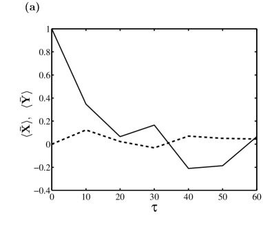
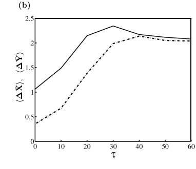
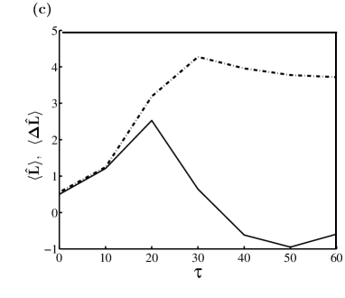
FIG. 2.: Plots of (a) $\langle\bar{X}\rangle$, $\langle\bar{Y}\rangle$, (b) $\langle\Delta\bar{X}\rangle$, $\langle\Delta\bar{Y}\rangle$, ($\bar{X}$ solid, $\bar{Y}$ dashed), and (c) $\langle\hat{L}\rangle$, $\langle\Delta\hat{L}\rangle$, (solid, dashed), for Simulation 2 where the initial state is a minimum uncertainty state offset from the origin.

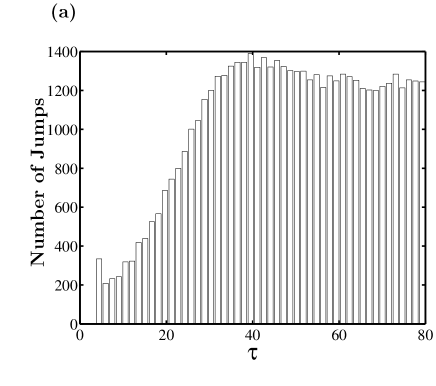
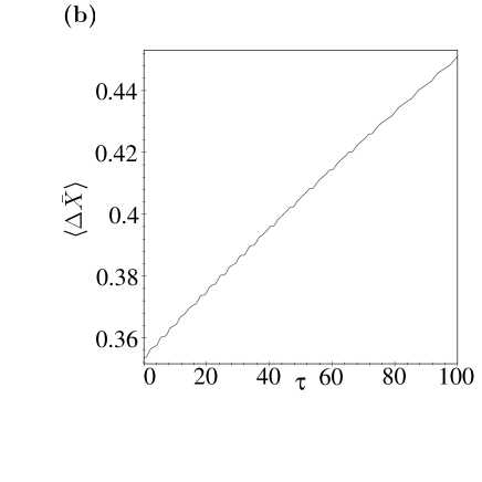
FIG. 4.: Plot (a) is the histogram of jump frequencies for Simulation 2, i.e. numer of jumps which occurred between time $\tau$ and $\tau+5$, while (b) plots $\langle\Delta\bar{X}(\tau)\rangle$ as an analytic comparison to Simulation 1. Here we have neglected the cross terms and recoil momentum kick in the master equation. This is solved analytically. See Appendix D for details.

REFERENCES

• [1] N. B. Simpson, L. Allen and M. J. Padgett, J. Mod. Opt. 43, 2485 (1996); V. E. Lembessis, L. Allen and M. Babiker,β€œOrbital angular momentum effects on atoms: A density-matrix theory”, in Coherence and Quantum Optics, eds. Eberly, Mandel and Wolf, (Plenum, NY 1996).
• [2] H. He, M. E. J. Friese, N. R. Heckenberg and H. Rubinsztein-Dunlop, Phys. Rev. Lett. 75, 826 (1995); M. E. J. Friese, J. Engler, H. Rubinsztein-Dunlop and N. Heckenberg, Phys. Rev. A 54, 1593 (1996).
• [3] M. Schiffer, G. Wokurka, M. Rauner, S. Kuppens, T. Slawinski, M. Zinner, K. Sengstock, W. Ertmer, β€œHolographically designed light-fields as elements for Atom Optics”, in IQEC ’96 Technical Digest, Sydney, Australia, (Optical Soc. America, ISBN 1-55752-459-9, 1996).
• [4] M. Babiker, V. E. Lembessis, W. K. Lai,L. Allen, Opt. Commun. 123, 523 (1996).
• [5] H. Ito, T. Nakata, K. Sakaki, W. Jhe and M. Ohtsu, β€œExperiments on atom guidence with evansecent waves”, in IQEC ’96 Technical Digest, Sydney, Australia, (Optical Soc. America, ISBN 1-55752-459-9, 1996).
• [6] G. A. Turnbull, D. A. Robertson, G. M. Smith, L. Allen and M. J. Padgett, Opt. Commun. 127, 183 (1996).
• [7] C. Tamm and C. O. Weiss, J. Opt. Soc. Am. B7, 1034 (1990); M. W. Beijersbergen, L. Allen, H. E. L. O. van der Veen and J. P. Woerdman, Opt. Commun. 96, 123 (1993).
• [8] N. R. Heckenberg, R. McDuff, C. P. Smith and A. G. White, Optics Lett. 17, 221 (1992); N. R. Heckenberg, R. McDuff, C. P. Smith, H. Rubinsztein-Dunlop and M. J. Wegener, Opt. and Quant. Elec. 24, S951 (1992).
• [9] S. J. van Enk and G. Nienhuis, Opt. Commun. 94, 147 (1992).
• [10] W. L. Power, L. Allen, M. Babiker and V. E. Lembessis, Phys. Rev. A 52, 479 (1995).
• [11] S. Dyrting, Phys. Rev. A 53, 2522 (1996).
• [12] A. P. Kazentsev, G. I. Surdutovich and V. P. Yakovlev, Mechanical Action of Light on Atoms, (World Scientific, Singapore, 1990).
• [13] A. P. Kazantsev, V. S. Smirnov, A. M. Tumaikin and I. A. Yagofarov, Opt. Spectrosc. 58, 303 (1985).
• [14] L. Allen, V. E. Lembessis and M. Babiker, Phys. Rev. A 53, R2937 (1996).
• [15] S. J. van Enk and G. Nienuis, J. Mod. Opts. 41, 963 (1994).
• [16] R. A. Beth, Phys. Rev. 50, 115 (1936).
• [17] N. B. Simpson, K. Dholakia, L. Allen, and M. J. Padgett, Opt. Lett. 22, 52, (1997).
• [18] J. Dalibard, Y. Castin and K. MΓΈlmer, Phys. Rev. Lett. 68, 580 (1992).
• [19] W.Β H. Press, B.Β P. Flannery, S.Β A. Teukolsky and W.Β T. Vetterling, Numerical Recipes, (Cambridge University Press , Cambridge, 1990).
• [20] M. Holland, S. Marksteiner, P. Marte and P. Zoller, Phys. Rev. Lett. 76, 3683 (1996).
• [21] M. Wilkens, E. Schumacher and P. Meystre, Opt. Commun. 86, 34 (1991).
• [22] R. M. Wilkox, J. Math. Phys. 8, 962 (1967).
• [23] I. S. Gradshteyn and I. M. Ryzkih, Tables of Integrals, Series, and Products, (Academic Press, London, 1980), section 9.100.
• [24] H. F. Dowker and J. J. Halliwell, Phys. Rev. A 46, 1580 (1992).
• [25] L. Allen, M. Babiker and W. Power, Opt. Commun. 112, 141 (1994).