The Quantum jump approach to dissipative dynamics in quantum optics
Abstract
Dissipation, the irreversible loss of energy and coherence, from a microsystem, is the result of coupling to a much larger macrosystem (or reservoir) which is so large that one has no chance of keeping track of all of its degrees of freedom. The microsystem evolution is then described by tracing over the reservoir states, resulting in an irreversible decay as excitation leaks out of the initially excited microsystems into the outer reservoir environment. Earlier treatments of this dissipation described an ensemble of microsystems using density matrices, either in Schrödinger picture with Master equations, or in Heisenberg picture with Langevin equations. The development of experimental techniques to study single quantum systems (for example single trapped ions, or cavity radiation field modes) has stimulated the construction of theoretical methods to describe individual realizations conditioned on a particular observation record of the decay channel, in the environment. These methods, variously described as Quantum Jump, Monte Carlo Wavefunction and Quantum Trajectory methods are the subject of this review article. We discuss their derivation, apply them to a number of current problems in quantum optics and relate them to ensemble descriptions.
Contents
toc
I Introduction
Quantum mechanics is usually introduced as a theory for ensembles, but the invention of ion traps , for example, offers the possibility to observe and manipulate single particles, where observability of quantum jumps, which are not be seen directly in the ensemble, lead to conceptual problems of how to describe single realizations of these systems. Usually Bloch equations or Einstein rate equations are used to describe the time evolution of ensembles of atoms or ions driven by light. New approaches via conditional time evolution, given say when no photon has been emitted, have been developed to describe single experimental realizations of quantum systems. This leads to a description of the system via wave functions instead of density matrices. This conditional ”quantum trajectory” approach is still an ensemble description, but for a sub ensemble where we know when photons have been emitted.
The jumps that occur in this description can be considered as due to the increase of our knowledge about the system which is represented by the wave-function (or the density operator) describing the system. In the formalism to be presented one usually imagines that gedanken measurements are performed in a rapid succession , for example, on the emitted radiation field. These will either have the result that a photon has been found in the environment or that no photon has been found. A sudden change in our information about the radiation field (for example through the detection of a photon emitted by the system into the environment) leads to a sudden change of the wave-function of the system. However, not only the detection of a photon leads to an increase of information but also the failure to detect a photon (i.e. a null result). New insights have been obtained into atomic dynamics and into dissipative processes, and new powerful theoretical approaches developed. Apart from the new insights into physics these methods also allow the simulation of complicated problems, e.g., in laser cooling that were completely intractable using the master equation approach. In general it can be applied to all master equations that are of Lindblad form, which is in fact the most general form of a master equation.
This article reviews the various quantum jump approaches developed over the past few years. We focus on the theoretical description of basic dynamics and on simple instructive examples rather than the application to various numerical simulation methods.
Some of the topics covered here can also be found in earlier summaries [Cook4, Erber2, Molmer3] and more recent summer school lectures [Knight1, Molmer2, Zoller2].
II Intermittent Fluorescence
Quantum mechanics is a statistical theory which makes
probabilistic predictions of the behaviour of ensembles (an
ideally infinite number of identically prepared quantum systems)
using density operators.
This description was completely sufficient for the first
60 years of the existence of quantum mechanics because it was
generally regarded as completely impossible to observe and
manipulate single quantum systems. For example, Schrödinger,
in 1952 wrote [Schroedinger1].
… we never experiment with just one electron or atom or
(small) molecule. In thought-experiments we sometimes assume
that we do; this invariably entails ridiculous consequences.
{…} In the first place it is fair to state that we are
not experimenting with single particles, any more than we can
raise Ichthyosauria in the zoo.
This (rather extreme) opinion was challenged by a remarkable idea
of Dehmelt which he first made public in 1975 [Dehmelt1, Dehmelt2].
He considered the problem of high precision spectroscopy, where
one wants to measure the transition frequency of an optical
transition as accurately as possible, e.g., by observing the
resonance fluorescence from that transition as part (say) of an
optical frequency standard.
However, the accuracy of such a measurement is fundamentally
limited by the spectral width of the observed transition. The
spectral width is due to spontaneous emission from the upper
level of the transition which leads to a finite lifetime
of the upper level. Basic Fourier considerations then
imply a spectral width of the scattered photons of the order
of . To obtain a precise value of the transition
frequency, it would therefore be advantageous to excite a metastable
transition which scatters only a few photons within the measurement
time. On the other hand one then has the problem of detecting these few
photons and this turns out to be practically impossible by
direct observation. So obviously one has arrived at a major dilemma here.
Dehmelt’s proposal however suggests a solution to these problems,
provided one would be able to observe and manipulate single
ions or atoms which became possible with the invention of single ion
traps [Paul1, Paul2] (for a review see [Horvath1]. We illustrate
Dehmelts idea in its original simplified rate equation picture. It
runs as follows.
Instead of observing the photons emitted on the metastable
two-level system directly, he proposed to use an optical double
resonance scheme as depicted in Fig. 1. One laser drives
the metastable transition
while a second strong laser saturates the strong
; the lifetime of the upper level is for
example while that of level is of the order of .
If the initial state of the system is the
lower state then the strong laser will start to excite the
system to the rapidly decaying level , which will then lead to the
emission of a photon after a time which is usually very short
(of the order of the lifetime of level ). This emission restores
the system back to the lower level ; the strong laser can
start to excite the system again to level which will emit a photon
on the strong transition again. This procedure repeats until at
some random time the laser on the weak transition manages to
excite the system into its metastable state where it remains
shelved for
a long time, until it jumps back to the ground state either by
spontaneous emission or by stimulated emission due to the laser
on the -transition. During the time the
electron rests in the metastable state , no photons will be
scattered on the strong transition and only when the electron
jumps back to state 0 can the fluorescence on the strong transition
start again. Therefore from the switching on and off of the
resonance fluorescence on the strong transition (which is
easily observable) we can infer the extremely rare transitions
on the transition. Therefore we have a
method to monitor rare quantum jumps (transitions) on the
metastable transition by observation of the
fluorescence from the strong transition.
A typical experimental fluorescence signal is depicted in
Fig. 2 [Thompson] where the
fluorescence intensity is plotted.
However, this scheme only works if we observe a single quantum system,
because if we observe a large number of systems simultaneously
the random nature of the transitions between levels and
implies that some systems will be able to scatter photons on the strong
transition while others are not because they are in their
metastable state at that moment. From a large collection of ions
observed simultaneously one would then obtain
a more or less constant intensity of photons emitted on the strong
transition. The calculation of this mean intensity is a straightforward
task using standard Bloch equations. The
calculation of single system properties such as the
distribution of the lengths of the periods of strong fluorescence,
required some effort which eventually led to the development
of the quantum jump approach. Apart from the interesting theoretical
implications for the study of individual quantum systems, Dehmelt’s
proposal obviously has important practical applications. An often
cited example is the realization of a new time standard using a
single atom in a trap. The key idea here is to use either the instantaneous
intensity or the photon statistics of the emitted radiation on the
strong transition (the statistics of the bright- and dark periods)
to stabilise the frequency of the laser on the weak transition.
This is possible because the photon statistics of the strong
radiation depends on the detuning of the laser on the weak
transition [Kim1, Kim2, Kim3, Ligare1, Wilser1]. Therefore a change in the
statistics of bright and dark periods indicates that the frequency
of the weak laser has shifted and has to be adjusted. However, for
continuously
radiating lasers this frequency shift will also depend on the intensity
of the laser on the strong transition. Therefore in practise
pulsed schemes are preferable for frequency standards
[Arecchi1, Bergquist2]
Due to the inability of experimentalists to store, manipulate and
observe single
quantum systems (ions) at the time of Dehmelt’s proposal, both the
practical as well as the theoretical implications of his proposal
were not immediately investigated. It was about ten years later
that this situation changed. At that time Cook and Kimble published
a paper [Cook2] in which they made the first attempt to
analyse the situation described above theoretically. Their
advance was stimulated by the fact that by that time it had
become possible to actually store single ions in an ion
trap (Paul trap) [Paul1, Neuhauser2, Paul2].
In their simplified rate equation approach Cook and Kimble started with the rate equations for an incoherently driven three level system as shown in Fig. 1 and assumed that the strong transition is driven to saturation. They consequently simplify their rate equations introducing the probabilities of being in the metastable state and of being in the strongly fluorescing transition. This simplification now allows the description of the resonance fluorescence to be reduced to that of a two state random telegraph process. Either the atomic population is in the levels and and therefore the ion is strongly radiating (on), or the population rests in the metastable level and no fluorescence is observed (off). They then proceed to calculate the distributions for the lengths of bright and dark periods and find that their distribution is Poissonian. Their analysis that we have outlined very briefly here is of course very much simplified in many respects. The most important point is certainly the fact that Cook and Kimble assume incoherent driving and therefore adopt a rate equation model. In a real experiment coherent radiation from lasers is used. The complications arising in coherent excitation finally led to the development of the quantum jump approach. Despite of these problems the analysis of Cook and Kimble showed the possibility of direct observation of quantum jumps in the fluorescence of single ions, a prediction that was confirmed shortly afterwards in a number of experiments [Bergquist1, Nagourney1, Nagourney3, Sauter1, Sauter2, Dehmelt3] and triggered off a large number of more detailed investigations starting with early works by Javanainen in [Javanainen1, Javanainen2, Javanainen3]. The following effort of a great number of physicists eventually culminated in the development of the quantum jump approach. Before we present this subsequent development in greater detail we would like to study in slightly more detail how the dynamics of the system determines the statistics of bright and dark periods. Again assume a three-level system as shown in Fig. 1. Provided the and Rabi frequencies are small compared with the decay rates, one finds for the population in the strongly-fluorescing level 1 as a function of time something like the behaviour shown in Fig. 3 (we derive this in detail in a later section.). We choose for this figure the values for the Einstein-coefficients of levels and reflecting the metastability of level 2. For times short compared with the metastable lifetime then of course the atomic dynamics can hardly be aware of level 2 and evolves as a 0 – 1 two-level system with the ”steady state ” population of the upper level. After a time the metastable state has an effect and the (ensemble-averaged) population in level 1 reduces to the appropriate three-level equilibrium values. The “hump” shown in Fig. 3 is actually a signature of the telegraphic fluorescence discussed above. To show this, consider a few sequences of bright and dark periods in the telegraph signal as shown in Fig. 4. The total rate of emission is proportional to the rate in a bright period times the fraction of the evolution made up of bright periods. This gives
| (1) |
but this has to be equal to the true average,
| (2) |
so that
| (3) |
and the ratio of the period of bright to dark intervals is governed, as we claimed, by the “hump”
So far, we have concentrated on situations where the Rabi frequencies are small (or for incoherent excitation). What happens for coherent resonant excitation with larger Rabi frequencies? The answer to this question is nothing [Knight3]: there are essentially no quantum jumps, at least at any significant level for coherently-driven resonantly excited three-level systems! But this is because of the idea of resonance is tricky: the strong Rabi frequency on the transition dresses the atom and the AC-Stark effect splits [Autler1, Knight2] the transition, forcing the system substantially out of resonance. If this is recognised and the probe laser driving the transition is detuned from the bare resonance until it matches the dressed atom resonance, then the jumps and telegraphic fluorescence return. We investigate this phenomenon more closely in Section V. As far as we know, the dependence of the telegraph fluorescence on detuning for coherently excited transitions has yet to be confirmed experimentally.
Let us return to the idea of a null measurement. We imagine that we observe the fluorescence from a driven three-level ion over a time scale which is long compared with the strongly fluorescing state lifetime but very short compared with the shelf state lifetime so that Pegg and Knight [Pegg3, Pegg3b] have shown that the average period of brightness and darkness in the telegraphic fluorescence can be obtained very straightforwardly from considerations of null detection. During such an interval the population in the shelf state, hardly has time to evolve, but population can be rapidly cycled from the ground state to the strongly-fluorescing state and back. Detection of a photon at the beginning of a interval implies a survival in the 0 – 1 sector for the whole interval and a bright period, whereas a null detection is sufficient for us to be confident that the atom is shelved for the whole interval and a dark period ensues.
If we take our origin of time to be after an interval in which we see a photon, then We can introduce the “life expectancy” as the time the atom spends in the 0 – 1 sector continuously. If the atom is still in this sector at a time (known from an observation of another fluorescence photon just prior to ), then the life expectancy will be also be So we can partition the outcomes into the case where at it has survived in the 0 – 1 sector with probability and the case where the ion did not survive the whole interval continuously in the 0 – 1 sector [Pegg3, Pegg3b]
| (4) |
where is a fraction Then for small
| (5) |
and if is small so we may neglect the possibility of a return from state back in to the 0 – 1 sector, so that
| (6) |
This is finite, so we know that the fluorescence will terminate. To obtain a value for we merely need to know the evolution equation (not its solution) for the population in state this would be the Bloch equation for coherent excitation, or the Einstein rate equation for incoherent excitation.
The calculation of the mean period of darkness proceeds along similar lines: if no photons are detected in an interval just before we find
| (7) |
The analysis presented here obviously also applies for the density operator equations in exactly the same form and we obtain
| (8) | |||||
| (9) |
Here the dot means the average gradient of the versus curve over a range of order . Because is much smaller than the characteristic change of it is very close to the normal derivative at all points.
It is straightforward to use this idea of ”collapse by non-detection” to estimate the characteristic time needed to be sure that a quantum jump has occurred [Pegg3b]. There are times as many short dark periods between photon emissions as there are prolonged dark periods of average length , where ( for strong transition saturation) is the average length of the short period. Thus the probability that an emission will be followed by a long dark period is approximately for , and the probability that it will be followed by a short dark period is close to unity.
Immediately following a photon emission, a dark period of length at least (with ) can exist for two complementary reasons: (a) the atom goes to state and therefore does not decay for a time of the order of , or (b) the atom is still in the plane but has not yet emitted a photon. The probability of (a) occurring is and the probability of (b) is approximately . Clearly for it is much more likely that any observed dark period of length is due to (b), but this becomes rapidly less likely as increases. The point where the observation of the dark period is just as likely to involve (a) as (b) is found by equating the two expressions to give
| (10) |
It follows that the sampling period must be greater than given by Eq. (10) this value in order for the observation of darkness during to imply (a) with reasonable certainty.
Further, because we know that immediately following the emission the atom is in , so the probability of being in is zero, and because Eq. (10) gives the order of the time of darkness required for the probability of being in to grow to about , Eq.(10) gives the characteristic time for the wave-function collapse by non-detection. This characteristic time can be associated with the time necessary for us to be certain that a quantum jump from to has occurred. For completely coherent excitation Eq. (10) reduces to an expression similar to that for the ”shelving time” found in [Porrati1] and in [Zoller1]. Note that while the collapse by non-detection of the system into the metastable state requires a finite time the collapse of the wave function due to the detection of a photon has to be viewed as practically instantaneous. When we detect a photon our knowledge of the system changes suddenly and this sudden change of knowledge is reflected by the sudden change of the system state which, after all, represents our knowledge of the system.
III Ensembles and shelving
Before we develop detailed theoretical models to describe individual quantum trajectories (i.e. state evolution conditioned on a particular sequence of observed events), it is useful to examine how the entire ensemble evolves. This is in line with the historical development as initially it was tried to find quantum jump characteristics in the ensemble behaviour of the system.We do this in detail for the particular three–level V–configuration (shown in Fig. 1) appropriate for Dehmelt’s quantum jump phenomena. For simplicity, we examine the case of incoherent excitation. Studies for coherent excitation using Bloch equations can be found , for example, in [Kim3, Kimble1, Ligare1, Nienhuis1, Schenzle2]. The Einstein rate equations for the V–system are [Pegg2]
| (11) | |||||
| (12) | |||||
| (13) |
where are the Einstein A- and B-coefficients for the relevant spontaneous and induced transitions, the applied radiation field energy density at the relevant transition frequency, and is the relative population in state ( for this closed system). In shelving, we assume that both and are much larger than and , and furthermore that . The steady–state solutions of these rate equations are straightforward to obtain, and we find
| (14) | |||
| (15) |
Now if the allowed transition is saturated
| (16) |
and
| (17) |
Now we see that a small transition rate to the shelf state has a major effect on the dynamics. Note that if the induced rates are much larger than the spontaneous rates, the steady state populations are the populations are evenly distributed of course amongst the constituent states of the transition.
However, the dynamics reveals a different story to that suggested by the steady state populations. Again, if the allowed transition is saturated, then the time–dependent solutions of the excited state rate equations tell us that for we have
| (18) |
and
| (19) |
Note that the these expressions are good only for strong driving of the transition. This especially means that for short times is of the order of which results in Eq. (19). Then for a very long–lived shelf state , we see that for saturated transitions ()
| (20) |
and
| (21) |
These innocuous–looking expressions contain a lot of physics. We remember that state is the strongly fluorescing state. On a time–scale which is short compared with , we see that the populations attain a quasi–steady state appropriate to the two-level () dynamics
| (22) |
This can of course be confirmed in an experiment [Finn1, Finn2]. For truly long times the third, shelving, state makes its effect and
| (23) |
as we saw qualitatively in Fig. 3. As we saw earlier in the discussion of Eq. (3), the change from two–level to three–level dynamics already gives us a signature of quantum jumps and telegraphic fluorescence provided we are wise enough to recognise the signs. Figure 3 illustrates the change from two to three–level dynamics.
The steady–state populations are sufficient to describe the average level of the fluorescent intensity. But how do quantum jumps and shelving show up in the intensity correlations? For example, let us examine the second order correlation function
| (24) |
where the colons describe normal ordering [Loudon1]. This correlation function is straightforward to compute from the Einstein rate equations using the quantum regression theorem [Lax1] which relates one-time to two–time correlations given the dynamics is Markovian. Here of course there are two intensities, that of the and of the fluorescence, so we can correlate the two light fields: ”1” with ”1”, or ”1” with ”2” and so on, where ”1” and ”2” represent the fluorescence on the and the transitions respectively. So let us concentrate on evaluating , which represents the joint probability of detecting a fluorescent photon () on the transition at time and some other photon (not necessarily the next photon) from transition at time . it is straightforward to show [Pegg2] that
| (25) | |||||
| (26) |
and
| (27) |
Using and that the transitions are saturated, then these correlation functions simplify to give
| (28) |
so that as expected, the correlation functions obey the same evolutions as the populations. It is worth noting that for short times we expect to see anti-bunching [Loudon1] from this three–level fluorescence, and this has been observed experimentally from trapped ions [Itano0, Schubert1].
In the mid 1980’s when studies of quantum jump dynamics of laser–driven three–level atoms began in earnest, a great deal of effort was expended in determining the relationship between joint probabilities of detection of a photon at time and the next or any photon a time later. This was addressed in detail by Cohen-Tannoudji and Dalibard [Cohen-Tannoudji1, Reynaud1], by Schenzle and Brewer [Schenzle1, Schenzle2] and others [Cook1, Lenstra1]. One attractive approach, advocated by Cohen-Tannoudji and Dalibard, uses a dressed manifold and from this evaluates the delay function describing the distribution of delay times before the next emission occurs. In Fig. 5 that laser excitation couples together these atom+field states, but fluorescence does not: spontaneous emission is an irreversible loss out of this manifold to states with reduced photon number in the excitation modes, but with photons created in initially un-occupied free-space modes.
We expand our atom+field state vector into the basis states with fixed number of fluorescence photons in the radiation field as shown in Fig. 5 as
| (29) |
and solve for the probability amplitudes . The probability of remaining without further emission in the -excitation atom+field manifold up to time is
| (30) |
The negative differential of this survival probability describes the delay function [Cohen-Tannoudji1]
| (31) |
so that the probability of there being an interval between one photon being emitted (detected) and the next is
| (32) |
To evaluate this interval distribution function it is sufficient to calculate the atom+field dressed state amplitudes. This demonstrates the utility of this approach: there is no need to solve the potentially complicated Bloch equations for the driven three–level atom, although of course this can be done [Schenzle2]. Kim and coworkers [Kim1, Kim2], Grochmalicki and Lewenstein (1989a), Wilser (1991) and later others have used the delay function to describe the shelving in the V system. The conditional probability of an atom emitting any photon between time and after emitting a photon at time is . The photon emitted at time can be the first to be emitted after that at or the next after any one at time (), so that
| (33) |
where is the interval distribution. If this is expressed in terms of its Laplace transform , then
| (34) |
The function is the normalized correlation function for a photon detection at followed by the detection of any photon (not necessarily the next) at time . It follows that
| (35) |
or equivalently in Laplace space
| (36) |
so that
| (37) |
For the case of incoherent, rate-equation excitation of a three–level V–system atom, it is straightforward to calculate the atom+field survival probability, differentiate this to generate the delay function and from Eq. (37) deduce . If this is done, precisely the same form is obtained as that from the quantum regression theorem. The merit of this approach is easier to appreciate for the case of coherent excitation, where the regression theorem requires the solution of the three–level Bloch equations and the solution of 8th order polynomial characteristic equations, compared with the need to solve three coupled equations, using the delay function route. In Section V we further illustrate the connection between the ”next” photon probability density and the ”any’ photon rate in Eqs. (215)-(226).
Rather than examine the correlation functions, it may be useful to examine other properties of the photon statistics, and in particular the variance in the photon numbers in the detected fluorescence [Kim1, Kim2, Kim3, Jayarao1]. For a Poissonian field, , but for a sub-Poissonian field , and for a super-Poissonian field, . To characterise the deviation from pure Poissonian fluctuations, Mandel [Mandel1] defined the parameter
| (38) |
which can be written in terms of the mean intensity and the second order correlation function as
| (39) |
If this is used to describe the fluorescence from a three–level atom involving shelving [Kim1, Kim2, Kim3] then as for saturated transitions
| (40) |
where are the mean times of bright and dark periods in the telegraphic fluorescence signal from the three-level atom shown in Fig. 1. If a dark period does not occur, whereas the larger becomes the larger the Mandel parameter becomes, reflecting the large fluctuations implicit in jumps from dark to bright periods. These macroscopic fluctuations are manifested in the photon counting distributions studied in detail by Schenzle and Brewer [Schenzle2] using Bloch equations. They showed that the count distribution of photons detected from the strongly allowed transition were Poissonian except for an excess of zero counts. In an interval of order of the lifetime of the shelving state one either counts a large number of photons (a bright period) or one counts nothing (a dark period). The probability of counting photons in time is Poissonian except again for an excess of zeros [Schenzle2] and is evaluated from the Mandel counting formula (or its quantum equivalent derived in [Kelley1])
| (41) |
except for . Here is the decay rate of the strongly-fluorescing state and is the detector efficiency. So in an interval where is the lifetime of the shelving state, we count either for typical transitions or we find . Note we essentially do not see as , as shown in Fig. 6. Schenzle and Brewer [Schenzle2] interpret these macroscopic intensity fluctuations in terms of quantum jumps. Imagine the fluorescent intensity to be jumping from dark (off) states to bright (on) states with probability distribution
| (42) |
then we find for the probability of counting photons in a time
| (43) |
where is the counting efficiency. The zero count is for saturated transitions. The behaviour of Eq. (43) is schematically shown in Fig. 6 where we see the excess probability for no counts (dark period) together with a high probability for a large number of jumps (bright period).
In the past two sections we have discussed the initial attempts towards a theoretical description of single ion resonance fluorescence. However, these attempts did not yet yield a satisfying approach to the problem as the single system properties described, e.g., by the delay function, were deduced from equations of motion describing the whole ensemble. In the next section we will now explain and summarize a number of approaches all giving the quantum jump approach that allows the most natural description of many properties of resonance fluorescence and time evolution of single quantum systems.
IV Discussion of different derivations of the quantum jump approach
A Quantum jumps
Prior to the development of quantum jump methods, all investigations
of the photon statistics started out from the ensemble description
via optical Bloch equations, or rate equations as presented above,
which were used to calculate nonexclusive ’probability densities’
for the emission of one or several photons at time in
the time interval . It is important to note that
only the probability of emission of any
photon was asked for. Therefore many more photons might have been
emitted in between the times . An example for
such a function which we discussed in section III is the intensity
correlation function
which gives the normalized rate at which one can expect to detect photons
(any photon rather than the next) at time when one has been
found at .
Efforts were made to use nonexclusive ”probability densities”
to deduce the
photon statistics of the single three-level ion and the aim was
to show that a single ion exhibits bright and dark periods in
its resonance fluorescence on the strong transition
[Pegg3, Schenzle2]. This approach is, however, not very satisfying
as it requires the solution of the full master equation and the inversion
of a Laplace transformation. Furthermore this approach is very indirect as
we first calculate the ensemble properties and then try to derive the
single particle properties. It would be much more elegant
to have a method which enables us to calculate the photon statistics
of the single ion directly. This was discussed widely at a workshop
at NORDITA in Copenhagen in December 1985, following a paper at that
meeting by Javanainen [Javanainen3]. This intention was finally
realized with the development of the quantum jump approach. Its development
essentially started when Cohen-Tannoudji and Dalibard (1986)
and much at the same time Zoller, Marte and Walls (1987) derived
the exclusive probability that,
after an emission at time , no other photon has been emitted
in the time interval [Cohen-Tannoudji1] or the
exclusive n-photon probability density
that in n photons are emitted exactly at the times
[Zoller1] without going back to the master equation
of the full ensemble. Both quantities are intimately related,
as the
probability density for the emission of the first photon
after a time is given by
| (44) |
and because it turns out that the exclusive n-photon probability density essentially factorizes into next photon probability densities
| (45) |
This factorization property was initially assumed and then justified by physical arguments by Cohen-Tannoudji and Dalibard in [Cohen-Tannoudji1] while in [Zoller1] first the exclusive n-photon probability was calculated and subsequently its decomposition into next photon probabilities was derived. Before we discuss the approaches of Cohen-Tannoudji and Dalibard [Cohen-Tannoudji1] and Zoller, Marte and Walls [Zoller1] we point out that although the exclusive (next photon at time ) and nonexclusive distributions (a photon at time ) are very different, they are related by a simple integral equation [Kim1]. We have, as discussed in Eq. (33) in Section III
| (46) |
which becomes especially simple as we saw when one considers the Laplace
transform of that equation as we have a convolution on the
right hand side of Eq. (46). This relationship enables us in
principle to obtain the exclusive probability density
from the nonexclusive quantity . In practice however this
is exceedingly difficult to do as one has to know all the
eigenvalues of the corresponding Bloch equations. Therefore a
direct approach is needed.
The idea put forward in [Zoller1] was to calculate not the
complete density operator irrespective of the number of
photons that have been emitted but to discriminate between
density operators corresponding to different numbers of emitted
photons in the quantized radiation field. The quantity of interest
is therefore
| (47) |
where is the density operator of atom and quantized radiation field, the partial trace over the modes of the quantized radiation field and the projection operator onto the state of the quantized radiation field that contains photons. This projector is given by
| (48) |
This method to calculate the density operator for a given number of photons in the quantized radiation field was first used by Mollow (1975) to investigate the resonance fluorescence spectrum of two-level systems. However, as at that time the investigation of single ions was completely beyond then-current experimental possibilities, so that he did not draw further conclusions from his approach concerning single quantum systems. This was only triggered later by the experimental realization of single ions in ion traps.
In the following we discuss the approach of Zoller et al (1987) for a three-level system in V configuration (see Fig. 1) case rather than as in the original paper for the two-level case. Following [Mollow1, Blatt1] one obtains for Eq. (47) the equations of motion
| (49) |
and
| (50) |
where the effective Hamilton operator is given by
| (51) |
with the detunings and, the laser frequency, the Rabi frequency and the Einstein coefficient on the transition. It is now important to note that the effective Hamilton operator is a non-Hermitean operator. The real part of is negative which implies that the trace of the density operator decreases in time. This is not surprising because describes the conditional time evolution under the assumption that no photon has been emitted into the quantized radiation field. The probability that an excited atom has not emitted a photon decreases in time and therefore the trace of describing this probability should decrease in time. This decrease is necessary for the trace of the density operator disregarding the number of emitted photons,
| (52) |
to be preserved under the time evolution. The equations of motion Eqs. (49) and (50) have the solution
| (53) |
where
| (54) |
and
| (55) |
with
| (56) |
From this result it is now possible to deduce the probability that exactly photons have been emitted in the time interval . The probability that no photon has been found should then be given by
| (57) |
and
| (58) |
is the probability that exactly photons have been emitted. Zoller, Marte and Walls then realized that the structure of these expressions coincides with that derived from an abstract theory of continuous measurement constructed by Srinivas and Davies [Davies1, Davies2, Davies3, Davies4, Srinivas1, Srinivas2]. This theory supports the interpretation of
| (59) |
as the probability density that exactly photons have been emitted at times and no photons in between. From the general theory of measurement, they interpreted the quantity
| (60) |
as the probability density that after an emission of a photon at time the next photon will be emitted at . It should be stressed that although in [Zoller1] the super–operator is identified with the time evolution of the ensemble irrespective of how many photons have been emitted in for the following it should always be chosen to be the time evolution if a given number of emissions have taken place at the times . Assuming this (as is also implicitly done later in [Zoller1]) one obtains for the probability density that photons are emitted exactly at times
| (61) | |||||
| (62) | |||||
| (63) |
Here we have factorized into products of
. In principle these functions can depend on the atomic
state at time (after the emission). However, in most cases
this state will be the ground state of the system and will be the same after
each emission.
Having found that the knowledge of is sufficient
( can be obtained via Eq. (44)), Zoller et al then continue
to discuss the photon statistics of the three-level V system. The results
found in [Zoller1] may also be used to implement
a simulation approach for the time evolution of a single three-level
system [Dalibard1, Dum1, Hegerfeldt1]. However, the application of the
quantum jump approach in numerical simulations will be discussed later in
this section.
The approach of Zoller, Marte and Walls already reveals many features
of the quantum jump approach. However there is a slight complication
in their approach as they rely on the abstract theory of
continuous measurement of Srinivas and Davies to give interpretations
to their expressions Eqs. (59)-(60). The reason that
they need the support of the theory of Srinivas and Davies is that they
never talk about the way the photons are measured.
In fact only the emission of photons is mentioned and not the detection
of photons. From a quantum mechanical point of view,
however, one has to be very careful, as the emission of
a photon is not well defined. It is the detection of a photon
in the radiation field which is a real event. Of course the treatment
in [Zoller1] already
implies some properties of the measurement process, e.g., they implicitly
assume time resolved photon counting. However, no explicit treatment
of such measurements was given in [Zoller1]. This problem was then
addressed in greater detail by several authors and in the following
we discuss these ideas.
The first approach to include the result of quantum mechanical measurements into their calculation explicitly was given by Porrati and Putterman (1989). They [Porrati1] as well as others [Pegg3] noticed that the failure to detect a photon in a measurement leads to a state reduction, as information is gained through that null measurement. Essentially we can be increasingly confident that the ion is in a non radiating state (examples of this will be shown in Section V). Porrati and Putterman assume that at some large time a measurement on the whole quantized radiation field is performed. Assuming the result of this measurement is the detection of no photons, they calculate all Heisenberg operators at that time projected onto the null-photon subspace of the complete Hilbert space, i.e., operators of the form
| (64) |
Although not mentioned explicitly in [Porrati1, Porrati2], the calculation of this operator turns out to be closely related to the projector formalism [Agarwal1, Haake1, Nakajima1, Zwanzig1], a connection that was elaborated on by Reibold [Reibold1]. Although their approach can in principle lead to the quantum jump method, there are some conceptual problems in the actual execution of the use of the null-measurements idea. The main problem is that Porrati and Putterman only talk about a single measurement at a large time performed on the complete quantized radiation field. This does not seem to be a very realistic model of measurements performed by a broadband counter, which informs us immediately whether he has detected a photon or not. Also the calculation of the state after the detection of a photon was not elaborated on in [Porrati1, Porrati2], where it was merely stated that the system is reset back to its ground state on photodetection which is of course a physically correct picture. These conceptual concerns to this approach were later addressed in the work of Hegerfeldt and Wilser [Hegerfeldt1, Wilser1], of Carmichael [Carmichael2] and of Dalibard, Castin and Mølmer[Dalibard1, Molmer1, Molmer2] and in the following we give a more detailed account of their approach.
We will follow closely the presentation given by the Hegerfeldt group [Hegerfeldt1, Wilser1] as it directly leads to the delay function that was also found in earlier papers [Cohen-Tannoudji1, Zoller1]. The physical ideas, however, are very similar to those presented elsewhere [Dalibard1, Molmer1, Molmer2]. We treat the same three level system as in the discussion of Zoller et al (1987).
In Hegerfeldt and Wilser (1991) and Wilser (1991) (as well as in [Dalibard1, Molmer1, Molmer2]), the following simple model of how the photons are detected was proposed. It was assumed that the radiating ion is surrounded by a –photodetector that detects photons irrespectively of their frequency and that the efficiency of the detector is unity. Efficiencies less than unity may be treated in a mathematically slightly different way using the same physical ideas [Plenio1, Hegerfeldt8] and leads to a natural connection between the next photon probability density and the any photon rate (intensity correlation function) [Plenio1, Kim1]. We will return to this point later. As truly continuous measurements in quantum mechanics are not possible without freezing the time evolution of the system through the Zeno effect [Mahler1, Misra1, Reibold2], it was instead assumed that measurements are performed in rapid succession where the time difference between successive measurements should be much larger than the correlation time of the quantized radiation field. This means that
| (65) |
If successive measurements are more frequent than we enter the regime of the quantum Zeno effect and we significantly inhibit the possibility of spontaneous emissions [Reibold2]. On the other hand should be much smaller than all time constants of the atomic time evolution to ensure that one finds the photons one by one and because we want determine the time evolution using perturbation theory. Therefore
| (66) |
For optical transitions it is easy to satisfy both inequalities Eqs. (65) and (66) simultaneously.
Now the density operator at time under the condition that no photons have been detected in all measurements which took place at time has to be calculated. Although the result of each measurement was negative, in the sense that no photon was found, this still has an impact on the wavefunction of the system, as it represents an increase of knowledge about the system [Dicke1, Porrati1, Pegg3]. Using the projection operator onto the vacuum state of the quantized radiation field and the time evolution operator of system and radiation field in a suitable interaction picture, we find
| (67) |
as, after each measurement which has failed to detect a photon, we have to project the quantized radiation field onto the vacuum state according to the von Neumann-Lüders postulate [Lueders1, Neumann1]. As obeys Eqs. (65) and (66), it is possible to calculate the time evolution operator in second order perturbation theory to obtain
| (68) |
with the effective Hamilton operator Eq. (51). In the quantum jump method presented in [Dalibard1, Molmer1, Molmer2] the Weisskopf-Wigner approach [Weisskopf1] was used to find a formula equivalent to Eq. (68). Inserting into Eq. (67) and going over from a coarse grained time scale to a continuous time, we obtain for the atomic part of the wavefunction (the radiation field is in its vacuum state) where no photons have been detected in all measurements in the interval
| (69) |
One should note that the effective time evolution does not preserve the norm of the state and that it maps pure states onto pure states. In fact the square of the norm of Eq. (69) is just the delay function
| (70) |
and coincides with given in Eq. (57). The delay function will become important in applications of the method in simulations [Dalibard1, Dum1]. It should be noted here in passing that if we consider the normalized version of the time evolution Eq. (69) for a two-level system, then one finds that it is identical to the time evolution according to the neoclassical radiation theory of Jaynes [Bouwmeester1]. The reason for this is claimed by Bouwmeester et al to rest on the fact that contains all contributions from virtual photons (i.e. all radiation reaction terms) but does not include the real photons as their detection leads to state reduction according to the projection postulate. However, neoclassical theory predicts quantum beats from a three-level system in configuration while it is easily seen that an analysis of the problem using the quantum jump approach does not predict quantum beats; a result in accordance with experiment Milonni (1976) and references therein.
Eventually the photo detector will find a photon and the state after this detection can be determined by the projection postulate. We write the state after the detection of a photon as a density operator, as the state after the emission can be a mixture (e.g. as in the three-level configuration [Javanainen4, Hegerfeldt3, Hegerfeldt6, Hegerfeldt9]) although in the case of the three-level V system it is not:
| (71) |
At this point the additional assumption is made that the photo detector absorbs the photon (which it does in reality) and that the state after the detection is simply obtained by removing the photons from the radiation field. This can be done by tracing over the quantized radiation field and multiplying with
| (72) | |||||
| (73) |
It should be noted that the assumption that the state after the
detection of a photon in the counter is given by Eq. (73)
is not included in the
projection postulate but enters as a physically justified
additional assumption. However using slightly different
mathematical methods it is possible to show that the procedure
Eq. (73) is not really necessary. Ideal quantum mechanical
measurements where the photon is not absorbed lead to the same
results [Plenio1, Hegerfeldt8]. This is a consequence of the intuitively
obvious fact that in free space photons emitted by the system will
never return to it and is implicit in the treatment of
Zoller et al (1987).
A different approach towards the quantum jump method was presented earlier
by Carmichael and coworkers [Carmichael1, Carmichael2].
They derive the quantum jump method from a discussion
of photoelectron counting distributions that are found in
experiments. A quantum mechanical theory for photoelectron
counting distributions was developed in 1964 by Kelley and Kleiner
[Kelley1] who derived the quantum mechanical expressions
for nonexclusive multicoincidence rates. For the probability to
have photoelectron counts in the time interval , they
find
| (74) |
where is the product of detector efficiency and a factor to convert field intensity into photon flux. The notation means that all operators have to be normally ordered and time ordered in such a way that times decrease from the centre towards the left and right. Expanding Eq. (74) one can write as a complicated series of integrals over the nonexclusive multicoincidence rates
| (75) |
which gives the rate for the joint detection of photons at times . It is a nonexclusive rate as there may be more detections in between the times . That these possible events are included in Eq. (75) is obvious, as the Heisenberg operators are calculated with respect to the total Hamiltonian of the system which describes a time evolution in which arbitrarily many photons may be created. The analysis of the photon statistics by means of the coincidence rate Eq. (75) has long been the standard way of investigation. It was, however, realized that this is not the only possibility, and for certain problems it is not even the most natural way. In fact Eq. (74) , for example, can be expressed very easily by the exclusive probability density to find photon counts at exactly the times and at no other time in . One finds for this the expression
| (76) |
Carmichael and coworkers [Carmichael1, Carmichael2] then undertook the step to express the exclusive probability density in terms of the intensity operators. They find
| (77) |
where
| (78) |
This can be checked by inserting Eqs. (77) and (78) into Eq. (76) and showing that the result coincides with Eq. (74) [Saleh1, Stratonovitch1]. The aim now is to rewrite Eq. (77) in terms of (super)-operators that only act in the atomic space, as these are much easier to handle than the Heisenberg-operators . It turns out that the resulting equations are quite simple. To this end it is important to note that the electric field operator in the Heisenberg picture can be decomposed into a free-field part and a source field part
| (79) |
In the Markov approximation the free field commutes with all electric field operators at earlier times Cohen-Tannoudji, J. Dupont-Roc, and G. Grynberg (1992) and when acting onto the vacuum state it vanishes. It is therefore possible to replace the intensity operators for by in Eq. (77). All other intensity operators remain unchanged. Carrying out the time ordering in Eq. (77) explicitly and after tedious calculations (for details we refer the reader to [Carmichael1, Carmichael2]) one obtains for an overall counter efficiency
| (80) |
where is the superoperator given by
| (81) |
where is obtained from for perfect efficiency
by substituting
. is the reset operator
giving the state after a photon has been detected. Assuming unit
efficiency () of the detection process we recover
Eq. (51).
So far we have discussed a number of approaches to the quantum
jump description of dissipation. These approaches can be formulated
somewhat
differently in the language of quantum stochastic differential
equations [Gardiner4]. This formulation is certainly rather
formal at first glance, but it has the advantage that certain
operations where one uses the Markov approximation become simpler.
On the other hand one has to use the somewhat unintuitive
Ito formalism [Gardiner4, Gardiner1] and a more physically oriented
derivation would sometimes be helpful for the interpretation
of the occurring equations.
To illustrate the idea of this formalism we consider a laser-driven
two-level atom in a quantized radiation field which is in the vacuum
state. We follow the description in Sondermann (1995b).
The Hamilton operator in a suitable interaction picture is given by
| (82) | |||||
| (83) |
where is an operator annihilating an electron in level and creating an electron in level and where
| (84) |
is the interaction energy between the electric-field operator in the Schrödinger picture (or more precisely in the chosen interaction picture) and the atomic dipole moment of the transition. The time discretized Schrödinger equation then reads
| (85) | |||||
| (86) |
where
| (87) |
We assume in the following that , which is crucial for us to be able to perform the Markov approximation. The idea is now to perform the Markovian limit directly in the Schrödinger equation instead of performing this limit on the results. This is the step where we have to introduce the notion of quantum stochastic differential equations, as in performing this limit we cannot subsequently interpret the resultant Schrödinger equation as an ordinary differential equation anymore [Gardiner4, Gardiner1]. Under the Markov assumption we have
| (88) |
which in the limit results in
| (89) |
We also need to know that if we assume that the initial state of the quantized radiation field is the vacuum, then
| (90) |
where this equation is defined in the mean-square topology sense, i.e., in brief one applies both sides on an initial vector and takes the absolute square of the result afterwards [Gardiner4, Gardiner1]. Taking the limit in Eq. (87) we have assumed the ordinary rules of calculus, and therefore generated a stochastic differential equation in the sense of Stratonovitch
| (91) |
As a Stratonovitch equation is not easy to integrate, we would like to transform it to an Ito-form using the rules Eqs. (88)-(90) [Gardiner4, Gardiner1]. We then find
| (92) |
where the arises from a
contribution. As the commute with
all earlier upon which depends, it can
be commuted to the right until it operates on the initial state
and therefore the vacuum. Therefore the contribution of the
vanishes and only the contribution survives.
What we are in fact interested in here is the rederivation of the
quantum jump approach. Therefore we are interested in the time
evolution when no photon is present in the field, i.e., we are interested
in the state vector
| (93) |
where is the projector onto the vacuum state of the quantized radiation field. We find
| (94) | |||||
| (95) |
The now vanishes because acting on a vacuum state to its left it gives zero contribution. The norm of the conditional state vector is just the probability to find no photon until if there was no photon at . This is just the reduced time evolution found in the previously discussed derivations other approaches, too. The probability density for an emission at time t is just the rate of decrease of the norm of the emission free time evolution, i.e.,
| (96) | |||||
| (97) | |||||
| (98) |
Therefore using this formulation we have recovered the quantum jump approach; we observe that this formalism, although not delivering new insights into physics different from those from previous derivations of the quantum jump approach, is very elegant from a formal point of view. To understand the formalism a little better, we now show how one may obtain Eq. (95) without referring to the formalism of stochastic differential equations [Zoller2]. We consider a finite time step for the state vector using the Hamilton operator Eq. (83) and first order perturbation theory. We obtain
| (99) | |||||
| (100) | |||||
| (101) |
where in the last line we have used the well known expression for the Heisenberg operator of the electric field operator which can be written as the free field contribution and a source term (the dipole of the atom radiates the outgoing field) [Loudon1]. Note that is now a Heisenberg operator. Eliminating in the last row of Eq. (101), as it operates on the initial vacuum state, we obtain
| (102) |
Now we may easily perform the limit to obtain the same result as in Eq. (95), however, without the explicit use of the quantum stochastic differential calculus.
B Quantum state diffusion and other approaches to single system dynamics
So far we have discussed the quantum jump approach for the description of single radiating quantum systems. The main ingredient in the derivation was the assumption of time resolved photon counting measurements on the quantized radiation field. The resulting time evolution could be divided into a coherent time evolution governed by a non Hermitean Hamilton operator which is interrupted by instantaneous jumps caused by the detection of a photon and the consequent gain in knowledge about the system. One could ask whether this description is unique, that is, it represents the only possibility. From the emphasis we put on the importance of the measurement process in the derivation of the quantum jump approach one can already guess that other measurement prescriptions will yield different kind of quantum trajectories. In the following we will discuss an important example, quantum state diffusion, [Gisin3] of a different kind of quantum trajectories which in fact can be derived from a very important measurement method in Quantum Optics, namely, the balanced heterodyne detection. Before we show the connection of quantum state diffusion to balanced heterodyne detection let us point out that quantum state diffusion was originally derived independently from a measurement context. Steps in this direction were made when several authors became interested in alternative versions of quantum mechanics [Pearle1, Ghirardi1, Ghirardi2, Diosi1, Diosi3] and the investigation of the wavefunction function collapse, i.e., the projection postulate [Gisin1, Gisin2]. In these investigations stochastic differential equations for the time evolution of the state vector of the system were studied. Again there is a multitude of possible equations; however, Gisin and Percival (1992a) provided a natural symmetry condition under which it is possible to derive a unique diffusion equation which is referred to as the quantum state diffusion model (QSD). Given a Bloch equation in Linblad form [Lindblad1]
| (103) |
with the system Hamiltonian , and the Lindblad operators , the quantum state diffusion equation for the state vector is
| (105) | |||||
The represent independent complex normalized Wiener processes whose averages, denoted by M(…), satisfy
| (106) | |||||
| (107) | |||||
| (108) |
Equation (105) has to be interpreted as an Ito stochastic differential equation, see , for example, [Stratonovitch1, Gardiner4]. It is easy to check that averaging Eq. (105) over the stochastic Wiener process yields the density operator equation Eq. (103) and that therefore (in the mean) normalization is preserved. For numerical studies often a somewhat simpler equation is used that does not preserve normalization even under the mean. This is given by
| (109) |
It should be noted that Eq. (108) is a nonlinear equation as it also depends on the expectation values of the Lindblad operators . This makes the analytical treatment of this equation very difficult and there are only a few cases for which an analytical solution is known [Gisin1, Gisin2, Salama1, Wiseman3, Carmichael4]. However it was found by Goetsch, Graham and Haake [Goetsch1, Goetsch2, Goetsch3] that it is possible to find linear stochastic differential equations which also reproduce the ensemble average. Stochastic differential equations for the wavefunction have also been derived by Barchielli [Barchielli1, Barchielli2, Barchielli3] (see also [Zoller2] for good summary of these approaches) from a more abstract mathematical point of view. The approach of Barchielli also gives a common mathematical basis for both diffusion and jump processes.
However, we do not intend to elaborate further on the mathematical side of the theory. Instead we would like to show that it is possible to derive QSD from the quantum jump approach in a certain limiting case, i.e., the case of infinitely many jumps where each jump has an infinitesimal impact on the wavefunction. In fact it turns out that QSD can be related to an explicit and well known physical measurement process in quantum optics, namely, the method of balanced heterodyne detection, see , for example, [Castin92, Wiseman1, Wiseman2, Wiseman4, Carmichael2, Molmer2, Knight1]. In the following we would like to show this explicitly for the specific example of a decaying cavity and we follow a similar path to that used in the approach of Garraway and Knight [Castin92, Garraway3, Knight1]. To be specific we will illustrate the method for the case of balanced heterodyne detection of the output of an undriven optical cavity. We have in mind the situation given in Fig. 7.
The left hand cavity A (with mode operators ) is the source a weak output field (mode operators ) which we want to analyze, while the lower cavity (mode operators ) is assumed to be in a coherent state with a very large amplitude for all times so that the radiated field (with mode operators ) of that cavity is very large. The Hamilton operator describing this situation is
| (111) | |||||
where the and are the coupling constants between the cavity and the outside world and and the frequencies of the cavity A and the local oscillator cavity respectively. The action of the beamsplitter is to mix the two incoming modes. Assuming a 50% beamsplitter we find for the new mode operators [Loudon2]
| (112) | |||||
| (113) |
Now going over to an interaction picture with respect to
| (114) |
and subsequently changing the basis via a displacement operator such that the initial state of the local oscillator is the vacuum [Mollow1, Pegg4] we obtain using
| (116) | |||||
Now applying the methods that we used to derive the quantum jump approach, we easily obtain the two jump operators
| (117) | |||||
| (118) |
where and are the decay rates of the cavity and the local oscillator. Within a short time interval , i.e., such that , we will count on average
| (119) |
counts in mode and
| (120) |
counts in mode where
| (121) |
These are average values around which the actual number of counts in the two counters fluctuates. We can approximate this number of counts by the stochastic process
| (122) |
such that . For the powers of the jump operators we find
| (123) | |||||
| (124) |
As we normalize after each emission the prefactors are not really important and we can divide the jump operators by these. One should note that the phase of these prefactors is fixed due to the fact that in the limit of infinite the jump operators have to become the unit operator. Therefore there is no freedom in the choice of the sign of the prefactors. It is now easy to derive the effective Hamilton operator for which we find
| (125) |
Using this together with Eq. (124) we obtain
| (126) |
Adding together the two Wiener noises , taking the limits and and defining
| (127) |
we obtain after dropping a counter-rotating term of the form
| (128) |
This is the unnormalized diffusion equation given , for example, by Gisin and Percival [Gisin3]. One should note that if we had considered homodyne detection, i.e., the case , then we would have found a different diffusion equation, as there would not have been a counter-rotating term which we could have dropped. Therefore an additional term in Eq. (128) would appear [Carmichael2, Molmer2].
To yield the normalized equations for QSD as they are given by Gisin and Percival (1992a) we have to normalize the wavefunction and we have to include a stochastic phase factor into the wavefunction [Garraway3] , i.e., we look for a diffusion equation for
| (129) |
The reason we have to include this seemingly unmotivated phase factor is that in the derivation of the QSD equation in [Gisin3], a term is added to the diffusion equation to give it the simplest possible form. This term in fact gives rise to a random phase change. To yield QSD we choose as
| (130) |
This choice has the effect of removing that would appear in the diffusion equation of the normalized wavefunction without the additional phase factor. Using Eq. (130) in Eq. (128) and assuming we finally obtain
| (132) | |||||
We have therefore shown that the quantum state diffusion equation Eq. (132) (or Eq. (105) ) can be regarded as a limiting case of the quantum jump approach. In Section V we will illustrate the transition from the quantum jump behaviour to the quantum state diffusion behaviour which takes place when we increase the amplitude of the local oscillator [Granzow96]. It should be noted that it is also possible to obtain a jump–like behaviour from quantum state diffusion equations. However, this procedure is much less satisfying than the above derivation of quantum state diffusion from quantum jumps. The reason is that one has to modify the quantum state diffusion equation by adding an additional operator, the localisation operator. The amplitude with which this localisation operator appears in the equations is arbitrary and has to be adjusted according to the experimental situation [Gisin9]. This is not particularly satisfying at least in cases in which we deal with single ion resonance fluorescence. Here the quantum jump approach appears to be much more natural. In fact it can be shown that one can not associate the jumps occurring in the quantum state diffusion picture with photon emissions as such an interpretation can lead to more than one emission from an undriven two-level system [Granzow96]. Taking these considerations into account one could be tempted to say that the quantum jump approach is more fundamental then quantum state diffusion. However, both approaches have the same justification as they were both derived from a particular measurement situation. Depending on the experimental situation and the measurement scheme employed we have to choose either the quantum jump approach or the quantum state diffusion model to obtain the correct description of the experimental situation. Quantum state diffusion was, as mentioned before, not originally introduced to describe a specific experimental situation. It was rather seen as an attempt to formulate alternative versions of quantum mechanics and there are attempts to derive diffusion equations from fundamental ideas such as , for example, decoherence induced by gravitational fluctuations [Percival2, Percival3, Percival4]. Although the quantum state diffusion model can not be regarded as the proper description of quantum jumps in single photon counting experiments but rather as the description of heterodyne detection it is nevertheless useful in the investigation of single system behaviour. Interesting phenomena such as localisation in phase and position space [Gisin6, Gisin7, Herkommer96, Percival1] are found. These can be used to improve the performance of simulation procedures using a ”moving basis” approach [Schack0, Schack1] where only time dependent subset of all basis states is used in the simulation. A similar method is also possible for a variant of the quantum jump approach [Holland2].
So far, we have discussed the evolution of open systems, that is of microsystems in contact with Markovian reservoirs such as the bath of vacuum field modes responsible for spontaneous emission. The quantum jump concept within an open system context has to do with the gain in information about the microsystem which is accessible from the record available in the dissipative environment. Such jump processes do not require an extension or modification of conventional quantum mechanics, and we refer to these as “extrinsic” jumps. A very different jump mechanism has been studied by a number of authors [Diosi3, Ghirardi1, Ghirardi2, Percival2, Percival3]. In these approaches the Schrödinger equation is modified in such a way that quantum coherences are automatically destroyed in a closed system by an intrinsic stochastic jump mechanism. This should be distinguished from the extrinsic mechanisms we are concerned with in the bulk of this review.
To see how an intrinsic jump mechanism works, we need a concrete realisation which we can apply to a specific time evolution. Milburn has proposed just such a realisation [Milburn3], in which standard quantum mechanics is modified in a simple way to generate intrinsic decoherence. He assumes that on sufficiently short time steps, the system does not evolve continuously under normal unitary evolution, but rather in a stochastic sequence of identical unitary transformations. This assumption leads to a modification of the Schrödinger equation which contains a term responsible for the decay of quantum coherence in the energy eigenstate basis, without the intervention of a reservoir and therefore without the usual energy dissipation associated with normal decay [Moya-Cessa1]. The decay is entirely of phase-dependence only, akin to the dephasing decay of coherences produced by impact-theory collisions or by fluctuations in the phase of a laser in laser spectroscopy, but here of intrinsic origin.
It is interesting to apply Milburn’s model of intrinsic decoherence to a problem of dynamical evolution: that is, the interaction of two subsystems and the coherences which establish themselves as a consequence of their interaction. In [Moya-Cessa1] the interaction between a single two-level atom and a quantized cavity mode was considered and shown how the intrinsic decoherence affects the long–time coherence characteristics of the entangled atom–field system. In particular it could be shown how the revivals (a signature of long–time coherence) are removed by this intrinsic decoherence. The quantum jump approach as we have discussed it so far only treats systems (atoms) interacting with a Markovian bath (the quantized multimode radiation field). However, one might be interested to apply the quantum jump approach to non Markovian interactions. Examples are electrons interacting with phonons or, in quantum optics, an atom in a cavity interacting with a mode which loses photons to the outside world [Garraway4]. The second example already suggests a possible way one could model such systems. Here the atom sees a cavity mode with finite width, i.e., a spectral function which is not flat but a Lorentzian (Piraux et al, 1990 and references therein. However, one does not need to solve a non Markovian master equation, as the width of the mode is produced by its coupling to the outside world. Taking this coupling explicitly into account, by describing a coupled atom-cavity field mode with a dissipative field coupling to the environment, one again obtains a Markovian master equation. This is also the recipe for the treatment of an interaction with a bath with a general spectral function [Imamoglu2]. One has to decompose into a sum (or integral) of Lorentzians with positive weights. Each Lorentzian can then be modelled by a mode interacting with both the system and a Markovian reservoir. This method is practical only if the number of additional modes that one has to take into account is not too large. One should also note that in this case the meaning of a jump in the simulation can become obscure, as the excitation of the system is transferred to the Markovian bath in two steps via the additional mode [Garraway4]. However, if one is only interested in a simulation method to obtain the master equation for non Markovian interactions this is not important.
We have discussed a number of derivations of the quantum jump approach so far. A different approach towards the description of single system dynamics has been proposed in [Teich1, Teich2]. In their method the dynamics described by the master equation is split into two distinct parts. One part changes smoothly the instantaneous basis of the density operator (coherent evolution) while the other part causes jumps between the basis states according to a rate equation. The instantaneous basis can be viewed as a generalisation of the dressed state basis. For a stationary state the basis states are fixed so that only jump processes occur. However, the approach is analytically quite complicated for nonstationary processes and in addition there are interpretational problems [Wiseman1].
At this point we would like to explain briefly a recently proven connection [Brun1, Yu1] between the quantum jump approach and a totally different concept, the Decoherent Histories formulation of quantum mechanics. A similar connection, although mathematically more involved, between the quantum state diffusion model and the Decoherent Histories approach has also been established [Diosi5]. The Decoherent Histories formulation of quantum mechanics was introduced by Griffiths, Omnès, and Gell-Mann and Hartle [Griffiths1, Omnes1, Omnes2, Omnes3, Gell-Mann1, Gell-Mann2]. In this formalism, one describes a quantum system in terms of an exhaustive set of possible histories, which must obey a decoherence criterion which prevents them from interfering, so that these histories may be assigned classical probabilities.
In ordinary nonrelativistic quantum mechanics, a set of histories for a system can be specified by choosing a sequence of times and a complete set of projections at each time , which represent different exclusive possibilities, i.e., they obey
| (133) | |||||
| (134) |
Note that the projection operators are Heisenberg operators; one could represent them in the Schrödinger picture by
| (135) |
The Schrödinger picture projection operators are assumed to be operators in the system space.
A particular history is given by choosing one at each point in time, specified by the sequence of indices , denoted for short. The decoherence functional on a pair of histories and is then given by
| (136) |
where is the initial density matrix of the system. The decoherence criterion is now given by this decoherence functional . Two histories and are said to decohere if they satisfy the relationship
| (137) |
where is the probability of history . A set of histories is said to be exhaustive and decoherent if all pairs of histories satisfy the criterion Eq. (137) and the probabilities of all the histories sum to .
To establish a connection between quantum jumps and Decoherent Histories the idea is to use a system that interacts with the outside world in one direction. An example of such a system is a cavity. The counter outside the cavity is now modelled by a two level system that is strongly coupled to a bath so that both its coherence as well as its excitation is damped much faster than all time constants of the evolution of the system. One then defines the two projection operators
| (138) |
These projections model the presence or absence of photons outside the system. It would be more general to consider more than one mode of the radiation field and the the proof can be generalised to that case. We now space these projections a short time apart, and each history is composed of projections representing a total time . A single history is a string , where represents whether or not a photon has been emitted at time . Using this, it is possible to write the decoherence functional as
| (139) |
where is the superoperator describing the time evolution according to the Bloch equations for the system (cavity) coupled to the two-level system. It is now possible to show that the decoherence functional in fact obeys Eq. (137) to a very good approximation. It should be noted that the construction of the decoherent histories using the two operators in Eq. (138) closely resembles the derivation of the quantum jump approach as given by Hegerfeldt and Wilser (1991) and Wilser (1991).
The crucial point in the quantum jump approach is the fact that we assume that we perform time resolved measurements on the photons that are emitted by the atom. These photons may be mixed with a local oscillator in a heterodyne detection as we did for the derivation of QSD but even there we assume time resolved measurements. A nice feature of the quantum jump approach has been that it allows us to describe the radiating system by a wavefunction instead of a density matrix. However, one may ask the question whether this is the only possible way to reach a wavefunction description of radiating systems. In fact it turns out that in some sense there is a complementary way to the quantum jump approach that also yields a wavefunction description. This method was proposed in [Holland1] and uses frequency resolved measurements instead of time resolved measurements. It turns out that again it is possible to decompose the density operator into pure states [Mollow1] which, however, are now characterized by the number of photons that have been detected and for which the frequency instead of their precise emission time is known.
C Simulation of single trajectories
After we have introduced and discussed different derivations of the quantum jump approach we will now briefly explain how the quantum jump approach is used to simulate single quantum systems. We will describe the simulation approach for a decaying undriven cavity. The generalization to an arbitrary system should then be obvious. Carmichael (1993a) has given a precise relationship between the conditioned density operator contingent on a precise sequence of detection events (a “record”) and the ensemble averaged density operator. He shows , for example, that if the zero temperature boson damping master equation is written in Liouvillian form
| (140) |
and we split the Liouvillian action as a sum of two terms, an anticommutator and a “sandwich” term,
| (141) | |||||
| (142) |
then we may identify the “sandwich” term as a jump operator. Equation (140) can be integrated formally as
| (143) | |||||
| (145) | |||||
where the quantity in curly brackets in Eq. (145) is labelled by Carmichael and is the conditioned density operator describing a specific “trajectory” or detection sequence. We can write in terms of the conditioned pure state projectors
| (146) |
The component propagates for a time without a decay being recorded: for the conditioned state
| (147) |
where the non-Hermitian effective Hamiltonian
| (148) |
derives from the anticommutator in Eq. (142). Once a decay is registered, the gain in information is responsible for the jump
| (149) |
The procedure adopted in quantum jump simulations can then be summarised as follows [Dalibard1, Dum1]:
-
1.
Determine the current probability of an emission:
(150) -
2.
Obtain a random number between zero and one, compare with and decide on emission as follows:
-
3.
Emit if so that the system jumps to the renormalised form:
(151) -
4.
Or no emission if so the system evolves under the influence of the non-Hermitian form
(152) -
5.
Repeat to obtain an individual trajectory, or history.
-
6.
Average observables over many such trajectories.
To reassure ourselves that this is all true, we note the history splits into two alternatives in a time
| (153) |
Then in terms of the density matrix, the evolution for a step becomes a sum of the two possible outcomes,
| (155) | |||||
| (157) | |||||
| (159) | |||||
so that
| (160) |
as in the original master equation Eq. (140). We have now seen how the quantum jump approach can be used to simulate a master equation. In Section V we will see some examples of such simulations and also of single realizations of quantum trajectories. After this simple approach to simulating the master equation we now give a brief exposition of the idea of higher order unravellings of the master-equation [Steinbach1]. To see the motivation we have to realize that the quantum jump approach is based on the simulation of the conditioned evolution of either a density operator or a state vector. However, at one point it is not a rigorous implementation of the trajectory concept. Because this method discretises time into small steps a quantum jump in the simulation takes a finite time whereas in a simulation of quantum trajectories the information gained from detection should instantaneously be used in conditioning the quantum state of the system. This pinpoints the subtle difference between conditioned trajectories and the slightly simpler idea of evaluating the probability of decay quanta at discrete timesteps. The simplest way to remedy the fact that conditioning takes time in the simulation is to add evolution with the effective Hamiltonian to the projection step that has to be performed when a photon is detected. Having said this, the question arises at what point during the time interval we need to condition the quantum state according to the result of the detection process. First, it is worth noting that wherever we decide to do this, it would not change the accuracy of integrating the master equation in first order. Second, we may try to increase the accuracy by choosing a specific point in the interval Let us integrate the master equation to second order in
| (161) |
Here is the Liouville operator describing the evolution of the complete master equation. The terms that result from evaluating the right hand side of this equation can be cast into the following form (for details see [Steinbach1]). By we denote the reset operator that has to be applied after the detection of a photon.
| (162) |
Here denotes evolution under the influence of the effective Hamiltonian
| (163) |
which we call the “no-jump” evolution. The four terms on the right hand side of Eq. (162) represent four specific conditioned evolutions or mini-trajectories that the system might follow. An expansion into mini-trajectories is important because only then can the density matrix evolution Eq. (162) be simulated with pure states. The first mini-trajectory in Eq. (162) represents evolution without any jump, the second and the third represent a jump followed by evolution without jumps and vice versa respectively and the fourth includes two successive jumps followed by no-jump evolution.
We see that it is not sufficient to specify one point in the interval at which to condition the density operator due to the quantum jump. We have to consider two points, at the beginning and at the end of and also the possibility of two immediately successive quantum jumps in order to increase the accuracy in by one order.
One can pursue this idea to obtain results which are accurate up to fourth order (in ). The master equation has to be integrated along the lines of a fourth-order Runge-Kutta method for ordinary differential equations. The result in fourth order then contains thirteen mini-trajectories (including the no-jump evolution) as follows
| (164) |
The subscripts on the non-Hermitian evolution indicate the fraction of the time interval for which each particular evolves the density operator, e.g., The way in which Eqs. (162) and (164) are turned into a Monte-Carlo simulation is clear: each mini-trajectory defines the conditioned evolution of the system and is assigned a specific probability with which it occurs, analogous to the jump and no-jump probabilities in the standard method. Just as in the standard procedure, a random number uniformly distributed between and is drawn to choose at random which of the mini-trajectories will govern the system evolution in the next timestep The no-jump evolution is tested first as this, for small is the most likely mini-trajectory. We note that the probability for evolution without detection remains unchanged as compared with the standard method and because the no-jump evolution is most likely the diversity of the mini-trajectories hardly influences the necessary computing time. However, if the no-jump mini-trajectory is not selected then one of the alternative trajectories in Eq. (164) must be chosen. For example, if the normalized state of the system at time is then the state of the system after evolution corresponding to the fourth mini-trajectory in Eq. (164) is,
| (165) |
which includes a renormalization factor The state is evolved with the effective Hamiltonian over two thirds of the timestep using a fourth-order Runge-Kutta integration step [Molmer1]. After projection with the Lindblad operator the evolution is continued with the non-Hermitian Hamiltonian for the remaining third of the timestep Only then is the resulting state vector renormalized. The probability for this mini-trajectory to occur is given by the product of the factor and the renormalization
To illustrate the improvement the method of higher order unravellings presents [Steinbach1] one can simulate a laser driven two-level system using the ordinary first-order (fourth order integration of the effective time evolution operator) and compare the result to the same simulation using the method of higher order unravellings. In Fig. 9 the simulation results of the inversion of the two-level system are plotted after runs and for a Rabi frequency equal to the Einstein coefficient of the transition, zero detuning and a time step . We clearly see that the first-order quantum jump approach (dashed line) deviates from the exact result (solid line) while the dotted line obtained from a fourth-order unravelling is much closer to the exact result.
D A quantum system driven by another quantum system
The next problem we want to investigate is that of a quantum system driven by the radiation emitted from another quantum system [Gardiner2, Carmichael3]. In the following we closely follow [Carmichael3]. One could try to solve the problem by determining the dynamics of the driving system first and from that the statistics of the emitted light. However, in general an infinite number of correlation functions is required to characterise the state of the light emitted from . In semiclassical theory one could instead simulate the properties of the light by implementing a suitable stochastic process, unfortunately this is not possible in the quantum case. Therefore it is better not to divide the problem into two but to determine the dynamics of the composite system . To obtain the broken time symmetry one uses an interaction between A and B that is mediated by a reservoir R and one assumes the Born-Markoff approximation. A simplified version of the problem is illustrated in Fig. 8 where it is assumed that only one mode of each cavity needs to be assumed. The cavities have three perfectly reflecting mirrors and one with transmission coefficient . The Hamiltonians and describe the free cavity modes and any interactions that take place inside the cavities. is the free Hamiltonian of a travelling wave reservoir R which couples the cavities in one direction only. The fields and that couple to the cavities are written in photon flux units. The complete Hamiltonian for is
| (166) |
with
| (167) | |||||
| (168) |
where and are the cavity linewidths, and and are annihilation operators for the cavity modes. describes two systems interacting with the same reservoir. It should be noted that and couple to that reservoir at different positions in space. Usually spatially separated reservoir fields are treated as independent an assumption that cannot be valid for the geometry shown in Fig. 8 where the output from cavity appears a time later at the input of cavity . The spatial separation of the two cavities can in fact be eliminated using the Born-Markoff approximation in the Heisenberg picture to relate and . One obtains
| (169) |
where
| (170) |
If is the density operator of system we may define the retarded density operator of the system as
| (171) |
and easily shows that satisfies the Liouville equation with the Hamiltonian
| (172) |
where
| (173) | |||||
| (174) |
Now and couple to the reservoir at the same spatial location and in addition they also couple directly with coupling constant . Now one can easily derive the master equation for the density operator of and obtains
| (175) |
with
| (176) |
Having found the master equation one can easily find the conditional time evolution that then allows to unravel the dynamics of the composite system . The time evolution of the conditional wave function between photodetections is governed by the Hamilton operator
| (177) |
After a photodetection we have to reset the system using the operator , i.e., . Now we are in a position to simulate individual trajectories of two coupled quantum systems. For applications of the theory , for example, to an atom driven by squeezed light or by antibunched light emitted from another atom see [Carmichael3, Gardiner2, Kochan1, Gardiner3]. An early example of an investigation of atoms driven by antibunched light was discussed by Knight and Pegg (1982).
E Spectral information and correlation functions
Until now we have discussed the quantum jump approach only in connection with quantities of the system or its resonance fluorescence that require a temporal resolution; no frequency information has been obtained as only broadband photon counting has been assumed. However, it would be nice to be able to use the quantum jump approach also for spectral properties of the resonance fluorescence of the system. Of special interest are , for example, the power spectrum of resonance fluorescence or the absorption spectrum of a weak probe laser. It turns out, that it is in fact possible to use the quantum jump approach [Gardiner1, Dum2, Molmer1, Mu1, Plenio1, Plenio2, Hegerfeldt8] and also quantum state diffusion [Gisin8, Sondermann1, Brun2, Schack1], to calculate those spectra. There are several different ways to derive quantum jump equations that enable us to calculate spectral information and in the following we will discuss three of them.
One possible approach can be made via the method of quantum stochastic differential equations (QSDE) [Gardiner1, Dum2]. We already outlined the spirit of their approach in Eqs. (83) - (102). Following essentially Gardiner et al (1992) but using the notation used in Eqs. (83) - (102) one defines an output mode operator
| (178) |
and then the spectrum in the Schrödinger picture as
| (179) |
where we defined
| (180) |
We can now introduce the auxiliary wave function
| (181) |
For these two wavefunctions one then obtains a Stratonovitch stochastic differential equation which can then be transformed into the Ito form. One then obtains
| (182) |
The spectrum is now by averaging
| (183) |
over many realization. Note that Eq. (182) for is just the conditional time evolution when no photons have been emitted. This equation is used to determine the jump times. The equation for has a free evolution similar to except for an additional rotation with frequency . In addition it is driven by . This driving can be interpreted as a process where a photon is emitted into the modes described by and where therefore the atom is deexcited. The approach given here can be used to simulate spectra in a number of situations [Dum1, Marte1, Marte2]. This approach is in fact similar in spirit to the approach of Schack et al (1996) who also assume the interaction of the system with one mode of the quantized radiation field. Schack et al then derive the quantum state diffusion equations that allow the calculation of the spectrum. It should be noted that using Eq. (182) and then following our derivation of quantum state diffusion from quantum jumps would have led to the same result.
A slightly different approach to the problem more in the spirit of the derivation of the quantum jump approach of [Hegerfeldt1, Wilser1] was undertaken in [Plenio1, Hegerfeldt8]. Their starting point is the photon number operator and they define the spectrum via the number of photons that have been emitted into certain narrow frequency intervals [Agarwal1] or to be more precise, the number of photons in a certain mode of the quantized radiation field (an approach using the electric field operator following similar lines is also possible and is essentially equivalent to the approach of [Gardiner1]). To remain close to a physical picture, they envisaged an experimental situation as depicted in Fig. 10. A part of the quantized radiation field (in a solid angle ) is observed by a broadband counter while in the rest of the space (solid angle ) a spectrometer (for example a Fabry-Perot) is situated.
The broadband counter performs time resolved observations on the quantized radiation field. It is again assumed that the time resolved measurements can be modelled by a sequence of gedanken measurements that are performed in rapid succession as in the derivation of the quantum jump approach [Hegerfeldt1, Wilser1]. At a large time , we then perform a spectrally resolved measurement of those photons that have entered the spectrometer. In that way one has measured a spectrum with a spectral resolution , which is conditioned on the particular detection sequence one has found in the broadband counter. The derivation of the relevant set of differential equations to calculate the spectrum follows similar ideas as they were developed in the work of Hegerfeldt and Wilser (1991) and Wilser (1991). The aim is to calculate differential equations for the conditional photon number in the mode which is given by
| (184) |
where , and we assume that is a vector pointing into the solid angle of the spectrometer. The conditional spectrum of resonance fluorescence is now obtained by summing over all vectors in . For the calculation of Eq. (52) we need the state where photons were detected at times only. With the projection operator onto the vacuum state for all modes with and with the abbreviation
| (185) |
where are the times of those measurements where no photon was found, we find, for ,
| (186) |
where is the state right after the detection of a photon in ; it is recursively given by
| (188) | |||||
Here denotes the partial trace over all modes
with a vector that points into the solid angle .
As in the usual quantum jump approach, at this point the assumption
enters that the photons detected in the broadband detector are
absorbed during the measurement as in a real counter. One can show,
however, that this assumption is not necessary for obtaining the
equations of motion used in this section [Plenio1]. In fact
one can just as well assume ideal quantum mechanical measurements
instead and obtain the same results [Plenio1]. This is of
course a manifestation of the intuitive physical idea that
photons emitted by the atom will not be reabsorbed as long as there
are no reflecting mirrors close to the atom. Mathematically it is
essentially a consequence of the Markov approximation which is
in the approach of Gardiner et al (1992) incorporated elegantly in the
formalism.
The general
principle is to find first the Heisenberg-Langevin equations
for operators of the form
| (190) |
where is the interaction picture time evolution operator. With the abbreviation
| (191) |
where and are defined similar to Eq. (79) without , we then find for Eq. (56)
| (192) |
Having found the Heisenberg-Langevin equations the next step is
to show that the occurring Langevin noise operators give a
negligible contribution. Having shown this one arrives at a set
of differential equations. As long as the solid angle covered by
the broadband counter is not equal to these equation
still describe mixtures as the photons emitted into the
spectrometer are not observed in a time resolved way. For the
explicit form of the equations of motion see [Plenio1, Hegerfeldt8].
Going over to the limit of a broadband counter
yields equations that maps pure states into pure states and which
are actually the same as those derived by Gardiner et al [Gardiner1].
The main ingredients in this derivation are the fact that the
initial state of the quantized radiation field is the vacuum
state and the Markov approximation.
Using this approach it is straightforward to derive the quantum
jump approach for the calculation of the absorption spectrum of
a weak probe beam by an atom. The idea is to assume that the
probe beam consists of a mode which is in a coherent state.
| (193) |
where
| (194) |
One then performs a unitary transformation that maps
this coherent state onto the vacuum state. This leads to
additional oscillating fields in the Hamilton operator and to an
initial state in the probe mode which is now the vacuum. Therefore the
approach
outlined above may be used again. Without further complicated
calculations one obtains the spectrum as the change in the photon
number in the probe mode. It is possible to show that this
definition of the absorption spectrum reduces to the stationary
absorption spectrum for sufficiently long times [Plenio1, Plenio2].
The approaches exhibited so far enable us to simulate spectral
information (e.g. the spectrum of resonance fluorescence). They were
derived for both a definition of the spectrum via the electric field operator
[Gardiner1] and via the photon number operator [Plenio1, Hegerfeldt8].
The physically motivated derivation of the formalism by Hegerfeldt and
Plenio [Hegerfeldt7, Plenio1] with a finite size spectrometer yields as a
byproduct equations of motion for a system that is observed by a counter that
does not cover the whole solid angle and/or has below unit efficiency.
These equations of motion will later be used to illustrate the connection
between
the next photon and the any photon probability and to show that an inefficient
photon counter will not measure the next photon probability but the any photon
probability which is proportional to the intensity correlation function
.
The approaches discussed so far gave equations that enabled
us to calculate the spectrum of resonance fluorescence directly
from the norm of a component of a propagated
’wave’function. However, there is a third way to obtain the spectrum of
resonance fluorescence which is via the simulation of the correlation function
(where is the Heisenberg operator corresponding
to )
and subsequent Fourier transformation of the
simulation results. Indeed this is the way in which
Dalibard, Castin and Mølmer [Molmer1, Molmer2] and others
[Garraway5, Mu1] employed the quantum jump approach to obtain simulations
of the spectrum of resonance fluorescence. The simulation procedure for a
correlation function of the form
runs as follows. First one evolves using
the MCWF approach a wave function towards .
Then one forms the auxiliary wave-functions
| (195) | |||||
| (196) |
where the are normalization constants. Now one has to evolve each of these four wave functions according to the MCWF procedure and then to form
| (197) | |||||
| (198) |
from which on obtains
| (199) |
It can be shown that this procedure produces the correct ensemble averages [Dalibard1]. A subsequent Fourier transform of the simulation results yields a spectrum. This procedure has been used , for example, [Garraway5] to simulate the spectrum of a three level system in a V configuration. However care has to be taken in this procedure because if one only performs a single Fourier transform to obtain the stationary spectrum
| (200) |
one inevitably runs into difficulties as one can only simulate finite times. Then, however, the Fourier transformation yields spurious negativities in in the power spectrum which are due to finite time effects. This problem can be circumvented by using a finite time double integral of the correlation function as required in the definition of the time dependent spectrum.
| (201) |
This quantity has the advantage that it is manifestly positive for each realization as it is of the form . However this considerably slows down the simulation procedure because the integral transform is now much more complicated.
A different point of criticism should be mentioned concerning the interpretation of a single run of this simulation procedure. While the derivation of the simulation procedure by Hegerfeldt and Plenio [Hegerfeldt8] clearly shows that a physical interpretation of a single run in the schemes derived in Hegerfeldt and Plenio (1996), Plenio (1994) and Gardiner et al (1992) is possible, although this is not obviously the case for the simulation procedure of Mølmer et al (1993) . A problem lies in the fact that four different wave functions have to be propagated in the procedure, each of which might follow different jump sequences. Furthermore even if only one jump sequence is followed, it is not clear what the interpretation of the correlation function is. This may be illustrated by the following example. We now would like to simulate a trivial correlation function of the form . We would expect that in each realization the simulation procedure would give the same result as for the single time expectation value . This, however, is not the case as is easily seen in the following example. We assume a spontaneously decaying TLS and the initial state
| (202) |
The emission–free time evolution is given by
| (203) |
where
| (204) |
If we assume that no jump at all occurs until we obtain according to the procedure of Mølmer et al (1993) the single run result for the correlation function to be
| (205) |
while for the expectation value of the operator at time is given by we obtain
| (206) |
These two expressions obviously differ. Therefore we can conclude that the simulation procedure of Mølmer et al (1993) yields the correct ensemble results; however if we are interested in questions concerning single runs or spectra conditioned on a given jump statistics care has to be taken and it is safer to resort to the approaches in [Gardiner1, Dum2] and Hegerfeldt and Plenio [Hegerfeldt8, Plenio1]. Applications to conditioned spectra will be given later in Section V.
Here we have only described in detail quantum jump approaches to calculate spectral information. Of course one can also obtain a quantum state diffusion simulation of spectral information. One can derive the equations either by starting out from the quantum jump equations given above and then follow our derivation of the quantum state diffusion equations as a result of heterodyne detection. Otherwise one can deduce the equations by assuming that the system couples to an additional output mode (i.e. similar to [Gardiner1] but here literally one mode of the quantized radiation field is chosen) and then writes down the master equation for that enlarged system. From that one can then easily obtain quantum state diffusion equations [Brun2]. However, if one tries to apply the equations to the calculation of time correlation functions of the form one again encounters interpretational problems similar to those explained for the approach of Mølmer described above. It should be noted that the approach to calculate time correlation functions given by Gisin (1993) does not lead to as usually defined in quantum optics but to a different correlation quantity which is difficult to interpret [Sondermann1].
V Applications of the quantum jump approach
A Photon statistics
In the previous sections we have introduced and discussed the quantum jump approach illuminating many different approaches to it. After these sometimes formal considerations we would like to give a number of examples to give a better understanding of the formalism and its physical implications. The examples will be drawn mainly from two physical situations; single trapped ions driven by lasers and electromagnetic fields in cavities, i.e., cavity QED.
We start by illustrating the difference between single realizations and ensemble averages by investigating a laser driven two–level system (TLS) damped by a zero temperature quantized radiation field. The master equation is then given by
| (207) |
with
| (208) |
where equals the Einstein coefficient of the observed TLS, the Rabi frequency and the detuning of the laser.
Assuming standard broadband photodetection, the quantum jump approach gives for the conditional time evolution between detections
| (209) |
with
| (210) |
and for the normalized state after the detection of a photon
| (211) |
The probability for not having a jump in the time interval if the initial state is the ground state, is given by
| (212) | |||||
| (213) |
with
| (214) |
Using the parameters and the upper state population of the ensemble evolves as shown in Fig. 11 where the initial state is the ground state. The population rises from zero, undergoing some Rabi oscillations and then tends towards a steady state. So much to the ensemble average. Now let us look at individual realizations of the time evolution using the same parameters and initial conditions. The result for one possible realization is shown in Fig. 12. The picture is strikingly different from Fig. 11 in that the time evolution is not smooth but exhibits jumps and it does not tend towards a steady state. We rather observe that initially the system starts to perform a Rabi oscillation. As the population in the upper level grows in time so does the probability for an emission of a photon. This oscillation is then terminated by the emission of a photon which brings the atom back to its ground state. Then the whole process starts again. Figs. 11 and 12 show little similarity; however, averaging over many individual realizations shown in Fig. 12 lead to a closer and closer approximation of the ensemble average. To illustrate this we have plotted the ensemble result together with the average over and individual realizations in Fig. 13. It is found that the root mean square deviation of the simulated average from the exact ensemble result are of the order of . We have examined the photon statistics of a two level system by detecting all the photons emitted by the atom with high time resolution as we assumed that the counter has unit efficiency and covers the whole solid angle. Assuming this, one would be able to measure the next photon probability density . However, in a real experiment the counter efficiency is much less than unity due to imperfect quantum efficiency and because only a finite solid angle is covered by the counter. Therefore the question is which function we actually measure when we perform a real experiment in which we determine the detection time of the ’next’ photon in our imperfect counter.
To answer this question we would like to employ the quantum jump approach assuming a perfect photon counter which, however, does not cover all space. If it covers a solid angle then this is equivalent to a counter of efficiency . The equation of motions for this setup up have been derived in section IV in connection with the simulation of spectral information (see Eqs. (184)-(192)). The efficiency of the detection process is the fraction of the emitted photons that are actually detected. We obtain the conditional equation of motion for the density operator under the assumption that no photon has been detected in the counter,
| (215) |
is given by Eq. (210) and one should note that now the conditional time evolution does not map pure states onto pure states. This is of course due to the incomplete information gained from the imperfect counter. Therefore we have to average over all possible events that the counter could not detect and this leads to a mixture. One observes two familiar limits: for zero counter efficiency we recover the ordinary optical Bloch equations, whereas for unit efficiency we find the effective time evolution inferred from the assumption that no photon has been found in the whole solid angle given a perfect counter.
Having found Eq. (215) we can now calculate the probability that the detector finds no photon in the time interval
| (216) |
which reduces to Eqs. (57) or Eq. (70) in the limit . The next count rate is then the negative time derivative of Eq. (216)
| (217) |
where is obtained by solving Eq. (215). Instead of solving this equation analytically we plot the solution for several different counter efficiencies . We assume and . In Fig. 14 we plot the next detection probability for counter efficiency and where the latter value of is computed from Mandels antibunching experiments [Kimble0, Dagenais1]. We observe that for decreasing counter efficiency the function Eq. (217) approximates the ”any photon” probability of the whole ensemble, which becomes more and more closely proportional to the intensity correlation function . So far we have we have shown how to calculate the next detection rate for different counter efficiencies from the quantum jump approach. We have plotted the results numerically. However it is also possible to derive an analytical expression in a somewhat different way. This was done in Kim et al (1987) and was in fact one earlier approach to the problem. As described earlier one can utilise the fact that there is a very simple relation between the ”any photon” rate of the complete ensemble and the next detection rate for a counter with efficiency . This relation can be found using
| (218) |
and
| (219) | |||||
| (220) |
where is calculated from Eq. (215). Inserting this and taking the Laplace transform this yields
| (221) |
The intensity correlation function is related to the any photon rate for an imperfect counting process by
| (222) |
Therefore we obtain
| (223) |
where is the Laplace transform of the intensity correlation function .
One should note that the intensity correlation function does not depend on the efficiency as it is normalized with respect to the stationary detection rate. From expression Eq. (223) one observes that, up to a normalization factor, the next photon probability tends towards the intensity correlation function. Inserting the well known expressions for the stationary state of the TLS and the intensity correlation function for zero detuning
| (224) |
and
| (225) |
into Eq. (223) we obtain
| (226) |
This Laplace transform can be inverted easily. Plotting this function exactly reproduces Fig. 14 if one normalises the maximum of to unity.
B Intermittent fluorescence
After this discussion of the photon statistics of the resonance fluorescence of a two-level system we now proceed to illustrate the formalism for a more complex system, namely, a three-level system in V-configuration as shown in Fig. 1. We assume that the transition is strongly allowed while the transition is metastable. In a typical experiment one would have a lifetime of the order of seconds for the metastable level , while the unstable level has a lifetime of several nanoseconds. The system is irradiated by two lasers, one on each transition. The Rabi frequency of the laser driving the transition is assumed to be much larger than the Rabi frequency on the transition. If one observes the intensity of resonance fluorescence on the strong transition under these conditions one typically obtains a result as shown in Fig. 2 or in a more schematical representation in Fig. 4. Long periods of brightness with many photon counts (bright periods) are interrupted by prolonged periods with no photo–detections (dark periods). As we discussed previously a simplified treatment of this situation using rate equations was given by Cook and Kimble [Cook2, Kimble1]. However, as the described situation involves lasers, a more detailed treatment is required as coherences can play a crucial role in the time evolution of the system. Such treatments were initially undertaken using Bloch equations but this is not the most natural description of the problem. Such a natural description of the problem was provided by the quantum jump approach. In the following we will use the quantum jump approach to calculate the photon statistics of the V-system and we will use it to gain interesting and sometimes surprising insights into the single system dynamics. It will turn out that the rate equation treatment of Cook and Kimble, while giving a qualitative picture, is insufficient to explain many interesting properties of the system. A similar analysis can be carried out for other systems such as a configuration [Agarwal3, Hegerfeldt6, Plenio1], and in a system where both upper levels couple strongly to the ground level but are close together [Hegerfeldt2, Hegerfeldt4, Hegerfeldt5, Koehler1].
In the following analysis we will always assume that both bright and dark periods are much longer than the lifetime of the unstable level . This condition is necessary from a physical point of view as otherwise one would not be able to distinguish between a dark period and the time interval between two successive emissions in a bright period. Also a bright period consisting of approximately one photon has little meaning. With the detuning and Rabi frequencies of the lasers on the transition we obtain the condition [Hegerfeldt7]
| (227) |
where equals the Einstein coefficient of level . This condition assumes that the Einstein coefficient of level is negligible. Again this can be cast into an analytical form. We require [Hegerfeldt7]
| (228) |
which expresses the fact that spontaneous emissions from level are much less frequent than stimulated transitions. This also implies that there are sufficiently many long dark periods.
To be able to calculate the mean lengths of bright and dark periods we need to define precisely what we mean by bright and dark periods. To distinguish between bright and dark periods we introduce a time . If our perfect photo detector fails to detect a photon in a time interval where it has found a photon at time we speak of a dark period of length . If, however, in a time interval the time between successive photon detections is always less than we have a bright period of length . Using these definitions and the next photon probability density we obtain for the mean length of a dark period
| (229) |
while the mean length of a bright period is
| (230) |
These expressions appear to be quite complicated but they can be simplified when we use the assumption that bright and dark periods are long compared to the lifetime of level . In that case it is obvious that the time evolution of the system has two widely different time scales, one determining the emission rate during bright periods, the other giving the rate at which dark periods occur. This is reflected in the fact that the probability to find no photon in the interval has a slowly decaying tail as we can observe from Fig. 15 where we plot for the parameters , and . If we chose such that it is much larger than the mean time between photon detections in a bright period while still being much shorter than the mean length of a dark period we can reliably distinguish between bright and dark periods. The choice of implies that
| (231) |
where is the smallest eigenvalue of the effective Hamiltonian of the system
| (232) |
Simplifying Eqs. (229) – (230) we then obtain
| (233) |
and
| (234) |
where is the mean time between successive photo–detections in a bright period
| (235) |
The mean time interval between successive emission in a bright period can be found from Eq. (235) or more easily from
| (236) |
where is the population of the upper level of a TLS driven by a laser of Rabi frequency and . Now it is quite easy to obtain analytical expressions for and . We find
| (237) | |||||
| (238) |
We see that under the conditions Eqs. (227-228) both bright and dark periods are much longer than the lifetime of the unstable transition.
Investigating the average rate at which we observe quantum jumps, i.e., the onset of dark periods, we see that it depends on the detuning of the laser on the transition. If we assume that the strong laser () is resonant () we observe that the ratio becomes minimal when and maximal for the Autler–Townes or Stark split detunings .
| (239) |
This dependence on the detuning reflects the fact that due to the strong driving of the transition the lower level exhibits Autler-Townes splitting. The two effective levels are shifted by with respect to the original level . To obtain long dark periods one needs to bring the weak laser on the transition into resonance with one of the dressed states of the transition. The resulting frequency dependence is shown in Fig. 16. Before we proceed with the investigation of the single system behaviour, we show again, now quantitatively, that the existence of bright and dark periods in the resonance fluorescence has a visible effect on the ensemble quantities, too. To see this, we plot the intensity correlation function in Fig. 17. We observe that there is a slowly decaying contribution for times quite similar to the behaviour of the next photon probability density shown in Fig. 15. One can show that in this regime we can approximate by
| (240) |
where and are given by Eqs. (237)-(238). Therefore from the measurement of the -function we can infer the existence of long bright and dark periods and one can determine their mean lengths. The fact that this information is hidden in the intensity correlation function is not surprising as it is proportional to the a photon rate which is related to the next photon rate via
| (241) |
Later we will also show that the existence of bright and dark periods also leaves its fingerprints in the spectrum of resonance fluorescence as well as in the absorption spectrum.
After this analytical discussion of the photon statistics of the V-system we will now investigate how the system time evolution for a single realization will typically look like. For the parameters and we have plotted both the time evolution of the population of the unstable level and population of the metastable level . In Fig. 18 one observes that in some regions a rapid change of accompanied by many detections takes place. However, there are also regions where no photon is found and most population is found in level while there is still a remnant in level . One should note that, as seen in Fig. 19 the population in level grows continuously and does not jump from level into level as one might expect from a rate equation picture. Nevertheless there is a jump, but not at the beginning of the dark period, but at its end [Wilser1, Garraway4] as we can see in Fig. 20 where we have magnified the time evolution of in a dark period. The jump occurs after a long time and marks the end of the dark period as after the jump the population is in the ground state which is strongly coupled to state . It should be noted that in the simulation shown in Figs. 18-20 the decay rate of the metastable level was assumed to be which implies that the dark period always ends with an emission from level . The continuous change of population towards the metastable state in a dark period nicely clarifies the importance of the failure to detect photons (null measurements) for the time evolution of the wavefunction. The failure to detect a photon provides us information about the system state which is described by the wave function. In this case the no-detection event tells us that we are more likely to find the system in the metastable state. Accordingly the wavefunction quickly (within several lifetimes of the unstable level) tends towards the metastable state if we have not found a photon for this time. The evolution is continuous as we assume (in the limit of the Markov approximation) continuous measurements of the radiation field. Therefore the failure to detect a photon in an infinitesimal time interval leads to an infinitesimal change proportional to . On the contrary the detection of a photon leads to a discontinuous change of the wave function because one quantum of energy has leaked out of the system into the environment. Therefore the system has to change discontinuously and jumps back into its ground state. Again this change of the wavefunction is due to our increased knowledge about the system.
C From quantum jumps to quantum state diffusion
So far we have only illustrated the quantum jump approach to the photon statistics of a single ion. In Section IV we have seen that other pictures are possible, namely, the quantum state diffusion picture. Instead of presenting a large number of examples for the quantum state diffusion model we rather want to illustrate how the transition from the quantum jump picture to the quantum state diffusion picture takes place. In Section IV we have seen how to derive the quantum state diffusion equations from a quantum jump description of a balanced heterodyne detection experiment. In this derivation we had to assume the limit in which the photon number in the local oscillator tends to infinity. In the following we will illustrate this limit by choosing a number of finite values for the photon number of the local oscillator. To keep the following short analysis as simple as possible we in fact do not consider the case of balanced heterodyne detection but of homodyne detection [Vogel1]. Instead of a cavity we will investigate the time evolution of a laser driven two-level system with upper level and lower level . We follow the presentation give in [Granzow96]. For the simulations we need to know two quantities. The Lindblad operator for the homodyne detection scheme is given by
| (242) |
where is the field amplitude of the local oscillator. As the Lindblad operator is changed and depends on so does the effective Hamilton operator between photon detections. We have
| (243) |
where equals the Einstein coefficient of the upper level , is the Rabi frequency on the transition and the detuning. The probability for a jump in the time interval is given by
| (244) |
These expressions can be derived analogously to the procedure that we applied in the description of the balanced heterodyne detection. In Fig. 21 we have plotted single realizations of a two-level system with Rabi frequency and local oscillators amplitudes a) , b) , c) and d) . One clearly observes that with increasing the number of jumps increase while their amplitudes decrease. For we already see a behaviour very close to that one would obtain in the limiting case .
D A decaying cavity
So far we have illustrated the quantum jump approach in the context of single ion resonance fluorescence. Now we would like to discuss a different kind of problem, namely, cavity QED [Haroche1]. That means we are interested in the field states inside a cavity as well as the time evolution of an atom interacting with such a cavity [Grochmalicki2, Imamoglu1]. Again these problems can be formulated in the framework of the quantum jump theory because both the losses of the cavity to the outside world as well as spontaneous emission of an atom give rise to a master equation of Lindblad form which can be simulated using wavefunctions. A derivation of the simulation equations is possible using the physical picture of photon counters surrounding the system. For example, a broad band photon counter outside the cavity will detect photon losses of the cavity. As an initial example to illustrate the physical insight that we gain from the quantum jump approach, we would like to investigate the time evolution of a field state in a lossy cavity. As an initial state we chose the state
| (245) |
In an appropriate interaction picture, the time evolution under the condition that no photon has been found by the photon counter outside the cavity is given by the effective Hamiltonian
| (246) |
while the normalized state after the detection of a photon is given by
| (247) |
In Fig. 22 the mean photon number for a single realisation is shown. Initially no jump takes place and the effect of this failure to detect a photon outside the cavity is that the mean photon number inside the cavity decreases; it becomes more and more unlikely to find a photon inside the cavity because if there was a photon in the cavity then it would leave the cavity, leading to a photon count. However, in the simulation shown in Fig. 22 we finally observe a photon outside the cavity and at that moment we know that there have been photons in the cavity. Calculating the state after the detection, given that we started with the superposition Eq. (245) we find that the post–detection state is a Fock state containing photons. This implies that the mean photon number after the photon detection is actually higher than before the detection. After this first detection, the cavity continues to decay and now each detection of a photon outside the cavity decreases the mean number of photons inside the cavity, while now the number of photons remains invariant under the conditional time evolution from the relevant Fock states.
In the previous example we saw that the exponential decay of the field mode in the ensemble average is the result of the superposition of many single realizations in which the cavity excitation changes discontinuously at random times. Coherence between component parts of a superposition state changes in amplitude and is eventually destroyed. However, this is not the only way in which coherence between superposition states is destroyed. In the following example we show that the decay of coherence of a Schrödinger cat of the form
| (248) |
is due to a randomisation of the relative phase between the two coherent states while the modulus of the relative phase remains invariant under the no–jump evolution [Garraway2]. In each individual realization the cat state remains a cat state. Although the amplitude of the two coherent states decays the relative phase between the two coherent states just changes its sign. In fact if the state before the detection is given by Eq. (248) then after the detection of a photon we have the state
| (249) | |||||
| (250) |
The conditional time evolution when no photon has been found is given by
| (251) |
so that the amplitudes of the coherent states decay exponentially while their relative phase remains unaffected. Averaging over many realizations, however, leads to a decaying relative phase as random phases tend to cancel out. It is interesting to note that the rate of decay for the relative phase of the Schrödinger cat is given by while the amplitude decay rate is given by . Therefore in the ensemble average the cat decoheres before the amplitudes of its constituents are significantly affected [Garraway3].
Another example that shows that the loss of coherence can be due to phase shifts at random times is the phenomenon of revivals in the Jaynes-Cummings model (Shore and Knight (1993) and references therein). In this phenomenon a two-level atom is initially in its excited state while the cavity field is in a coherent state with amplitude ,
| (252) |
This initial product state becomes entangled (Ekert and Knight (1995) and references therein) and the average excitation of the atom rapidly tends towards . The reason for this is the fact that the frequency of Rabi oscillations depends on the number of photons in the field mode [Narozhny1]. The different Rabi frequencies quickly decohere so that one observes an average excitation of of the atom. However, as the frequencies are discrete they partially rephase after a longer time and the excitation of the atom rises again. This revival is shown , for example, in Fig. 23. Revivals of this kind have been observed experimentally by [Meekhof1, Brune1] and of the micromaser kind by Rempe et al (1987). If the cavity is damped, however, these revivals are much weaker and will vanish for strong damping as shown in Fig. 24 where we have chosen the same parameters as in Fig. 23 but with an additional cavity damping constant of , where is the atom–field coupling constant. We assumed that the atom does not decay spontaneously. No substantial revivals can be observed [Barnett1]. What will we see for an individual realization? If we assume that the atom does not decay spontaneously we obtain the effective Hamiltonian
| (253) |
that generates the conditional time evolution of the atom cavity system if no photons are detected outside the cavity. generates the free evolution of an undamped atom cavity field system while the second term on the right hand side describes the damping of the cavity at a rate . The state after the detection of a cavity photon which is
| (254) |
A single realization for the parameters of Fig. 24 is shown as in Fig. 25. Now the revivals persist, however, each jump that occurs at a random time introduces a phase shift. An average taken over many individual realizations then leads to a quick decay of the coherence and revivals are not observed any more. A similar analysis can be performed for a lossless cavity with an atom that may spontaneously decay [Burt1].
In these examples we only considered undriven atoms in a cavity. Driven two-state systems inside a cavity can of course also be investigated using the quantum jump approach [Alsing91, Tian1] but we do not discuss this in detail here.
E Other applications of the quantum jump approach
So far we have illustrated the quantum jump approach for a number of examples in single ion physics and cavity QED. The quantum jump approach can and has been applied to a large number of problems which we cannot discuss in detail here. Amongst these examples are the discussion of correlations between quantum jumps in two stored ions. Such correlations were observed in an experiment [Sauter3] in which the intermittent fluorescence of two ions in an ion trap were investigated and correlations were found between the quantum jumps in the two ions exceeding those expected from independent jumps. However, Itano et al (1988) could not confirm these correlations in their experiment [Itano0]. Theoretical investigations [Agarwal2, Hendriks1, Lawande2, Lawande4, Lewenstein1, Lewenstein2] predicted that correlations should be small if the ions are separated by many optical wavelengths. If the ions are closer than an optical wavelength together, correlations might be observable. For such small separations even two two-level ions could exhibit quantum jumps [Yamada1, Kim4, Lawande5].
Another example of the application of the Quantum jump approach is the investigation of the Quantum Zeno effect [Misra1]. The Quantum Zeno effect was measured in an experiment by Itano et al (1990) which was originally proposed by Cook (1988). The experiment used a two-level system. The ground state population was measured via coupling the lower level strongly to a rapidly decaying third level. Observation of resonance fluorescence then indicates that the system was in its ground state. This experiment was investigated theoretically independently by Power and Knight [Power1, Power2, Power3], by Beige and Hegerfeldt [Beige1, Beige2] and by Mahler and coworkers [Mahler1] using the quantum jump approach and, e.g., by Frerichs and Schenzle (1991) using Bloch equations. The investigations using the quantum jump approach helped to understand the experiment from the single particle point of view and will be important in the analysis of future Quantum Zeno experiments [Plenio3] using single ions instead of around in the experiment by Itano et al (1990).
Cohen-Tannoudji and coworkers have applied the quantum jump approach to the problem of lasing without inversion [Cohen-Tannoudji4, Cohen-Tannoudji5, Cohen-Tannoudji3] to understand the processes involved from the point of view of single systems.
Apart from these more analytical applications of the quantum jump approach also its numerical usefulness has been demonstrated , for example, in numerical simulations of laser cooling experiments in two or three dimensions (see, for example, [Castin1, Marte1, Marte2]). It is the fact that the quantum jump approach allows the description of the system using a wave function instead of the density operator that made these investigations possible. Both the gain in computational speed and the saving in memory space is considerable as in a quantum jump simulation only differential equations have to be propagated instead of in the density operator simulation.
The quantum state diffusion model, apart from its importance in fundamental issues such as the measurement process or intrinsic decoherence, is now widely used to investigate the transition between classical and quantum behaviour and in the field of quantum chaos (see, for example, [Rigo96, Spiller1, Brun3]). As we have already mentioned in Section IV the quantum state diffusion model also exhibits interesting localisation properties in both position and phase space [Gisin6, Gisin7, Herkommer96, Percival1] which can be used to implement very fast simulation algorithms [Schack0, Schack1]. Similar localisation properties exist also for variants of the quantum jump approach [Holland2].
A more exotic application of the quantum jump approach, or more precisely of the experiments in which quantum jumps were observed, is the fact that these experiments can provide a ”perfect” random number generator. This is because these experiments allow the observation of single quantum jumps which occur at absolutely random times due to the fundamental indeterminacy of quantum mechanics [Erber1, Erber2]. Whether this idea is useful is, however, doubtful although in principle there could be applications, e.g., in cryptography.
F The spectrum of resonance fluorescence and single system dynamics
So far our examples of the quantum jump approach were limited to the investigation of the photon statistics of the radiation emitted by a system and of the internal dynamics of a system conditioned on the measurement record observing the radiation emitted by the system. As a further application of the quantum jump approach we would now like to consider the spectrum of resonance fluorescence of a three-level atom in the V-configuration as shown in Fig. 1. This system, whose photon statistics we already discussed in the context of bright and dark periods exhibits interesting features in the spectrum of resonance fluorescence on the strong transition. In the following we will discuss briefly the ensemble behaviour of the spectrum and then show how we can understand this behaviour from the point of view of the single system dynamics. We will closely follow the analysis in Hegerfeldt and Plenio (1995b) and Plenio (1994,1996). We consider the system shown in Fig. 1 and assume that the Rabi frequencies of the lasers and the decay constants of the two upper levels satisfy the following conditions.
-
The Rabi frequency of laser driving the transition is weak, that is
(255) which simplifies for to
(256) -
Spontaneous emission on the transition should be negligible, that is
(257)
These conditions have the following interpretation. If Eq. (255) is satisfied the V system exhibits long bright and dark periods as discussed in Eqs. (227) -(238). If Eq. (257) is satisfied stimulated transitions from level to level are much more frequent than spontaneous emissions on the same transition. Under the assumption of Eqs. (255)-(257) the spectrum of resonance fluorescence takes on the following approximate analytical form
| (258) | |||||
| (259) |
with
| (260) | |||||
| (261) | |||||
| (262) | |||||
| (263) | |||||
| (264) |
and
| (265) | |||||
| (266) | |||||
| (267) |
The contributions Eqs. (265) and (266) just represent the well known Mollow triplet and the Rayleigh peak [Mollow1, Mollow2, Mollow3, Mollow4, Mollow5]. These contributions are expected and are well–understood. The third contribution however, a narrow Lorentzian, is a new feature in the spectrum of resonance fluorescence. In Figs. 26 and 27 we see the spectra for the cases of strong driving of the transition and for a medium strong laser on the same transition. One clearly observes the narrow peak , which should not be confused with the Rayleigh peak, in both spectra. In the following we will focus our attention to this new feature and use it as an example for the application of the quantum jump approach for spectral information and to illustrate how ensemble properties can be understood better from a single system point of view. One might, for example, be interested in the following question. What happens if we observe the spectrum of resonance fluorescence in a bright period exclusively? Experimentally this may be measured by triggering the spectrometer with the broadband counter. The spectrometer will be opened if we detect photons in the broadband counter at a sufficiently high rate and it will be closed when we fail to find photons for a certain time . Using this time constant we have a means either to observe the spectrum in a bright period () or with no restriction on the emission times (), i.e., the ensemble spectrum. Changing we can continuously switch between the two regimes. The spectrum of resonance fluorescence can be simulated using the quantum jump approach [Hegerfeldt8]. In Fig. 28 the effect of the change in is clearly visible. For small the amplitude of the narrow central peak becomes small. However only the central part of the spectrum is strongly affected while the wings of the spectrum are more or less independent of . This is an example of conditional fluorescence spectra and it shows that spectra can be dependent on the conditions imposed on the photon statistics. Here we have shown the effect for the spectrum of resonance fluorescence but similar results may be obtained by investigating the absorption spectrum of a weak probe beam on the strongly driven transition [Plenio2]. Again a narrow peak is observed which vanishes if we try to measure the same feature in a bright period of the system. After we have investigated the spectrum of resonance fluorescence of the V system and some of its properties, especially the occurrence of the narrow peak, it is now instructive to see how we can understand this feature from the photon statistics of the single atomic system. The photon statistics are provided by the quantum jump approach. Explicit results have been given in this section in Eqs. (227) -(238).
Now that we know that the V configuration exhibit light and dark periods for those parameters for which the narrow peak in the spectrum appears we proceed with a somewhat simplified model of resonance fluorescence of the V-system. We assume that the lengths of light and dark periods obey exactly Poissonian distributions, e.g., the probability density that a light period has the length is
| (268) |
and for a dark period to have a length of is
| (269) |
These probability densities have been derived from a rate equation model of the time evolution by Cook and Kimble [Cook2]. Additionally we assume that in a bright period the system behaves exactly like a two-level system made up of the two levels and . This assumption has to be checked and turns out to be good in the case of the spectrum of resonance fluorescence treated here. However, it is not always correct as a careful analysis of the absorption spectrum on the strong transition proves and deviations from this idealised assumption may lead to significant contributions in the absorption spectrum [Plenio2].
It is well known [Loudon1] that the stationary spectrum of resonance fluorescence of such a two-level system is given by
| (270) |
where and denote the negative and positive frequency part of the electric field operator and is chosen in such a way that with
| (271) |
one obtains
| (272) |
For the nonnormalized resonance fluorescence spectrum of the two-level system one then obtains
| (273) |
where the constants and are given in Eqs. (260)-(262). As the light emitted by the atom switches on and off due to the light and dark periods we assume that the electric field radiated by the 3-level configurations is given by
| (274) |
where is a two state jump process with values 0 and 1. The probability density for the length of a period where is given by Eq. (268) and that for is given by Eq. (269). Therefore we have to substitute
| (275) |
in Eq. (272) and expect the spectrum of the three-level configurations to be given by
| (276) |
where denotes both the quantum mechanical average as well as the stochastic average over all realizations of the process . This can be simplified to
| (277) | |||||
| (278) |
with
| (279) | |||||
| (280) |
where
| (281) |
Because both and (Eqs. (236)-(238)) are assumed to be much longer than the mean emission time of a two-level system, which is of the order of , we can deduce from this
| (282) | |||||
| (283) |
This expression has to be compared with the results Eqs. (259)-(267). In fact inserting Eqs. (236)-(238) into Eq. (283) yields an expression in very good agreement with the spectra of the V-system. The width of the resulting narrow peak is
| (284) |
The amplitude of the narrow peak in the normalized spectrum is then given by
| (285) |
Now the interpretation of the narrow peak is obvious. The stochastic modulation of the resonance fluorescence due to dark periods leads to a partial broadening of the Rayleigh peak. The small width of the additional peak in the resonance fluorescence spectrum is then understood from the fact that the correlation time of the random telegraph process f(t) which simulates the light and dark periods is very large. In fact it is easy to show that
| (286) |
This results in an extremely narrow distribution in frequency space with a width . It is this structure which is observable in the spectrum of resonance fluorescence. It is interesting to note that the narrow peak is not easily interpreted in a dressed-states picture. Indeed, in secular approximation and for one obtains a zero weight for the narrow peak. Even if we tune the laser on the transition to resonance with one of the dressed states, i.e.. , the weight of the narrow peak comes out much too small. In fact it would then be predicted to be proportional to . The narrow peak found here has clearly a different origin than the line narrowing effects found by others [Manka1, Narducci1, Narducci2] where the systems do not exhibit bright and dark periods in their resonance fluorescence but simply a decrease in intensity. The existence of bright and dark periods in the resonance fluorescence leads to a narrow peak in the spectrum but it should be noted that the converse is not necessarily true. There are situations (eg a laser driven TLS in a squeezed vacuum [Swain1]) in which the spectrum of resonance fluorescence exhibits narrow peaks but where the photon statistics does not show bright and dark periods. The reason for that can be found in the fact that the photon statistics is governed by the population decay rates while the spectrum of resonance fluorescence is derived from the correlation function which is strongly influenced by the decay rates of the coherences in the system. In the case of a TLS in squeezed light the coherences have a slowly decaying component while the population decay rate is still large.
G Spontaneous emission in quantum computing
As a last application of the quantum jump approach we would like to investigate the influence that spontaneous emission has on the function of a quantum computer. Quantum computing is an idea that has attracted enormous interest in the last two years. It was elevated from the obscurity of theoretical idealisation to possible practical applications by the discovery of an algorithm by Shor (1994) (see also Ekert and Josza (1996) and references therein) that allows the factorization of large numbers in polynomial time on a quantum computer as compared to the exponential time required on a classical computer. However, this achievement in computing speed is only possible due to the massive use of the superposition principle in quantum mechanics. The basic idea is that a qubit (a two level system) can exist in a superposition of the two values and . qubits can then exist in a superposition of values. These values can then be manipulated by a series of unitary transformations. A final readout can then provide us with information about global properties of the function implemented by the unitary transformation. Such a global property of the function is, for example, its period which a quantum computer determines by performing a discrete Fourier transform, something which can also be implemented on a quantum computer [Coppersmith1]. In the course of its time evolution (computation) the quantum computer evolves into a highly entangled state. However, it is known that any entangled state is very sensitive to dissipation. Therefore one expects that the quantum computer is highly sensitive to spontaneous emission and other sources of dissipation. This is in fact the case and currently research in quantum error correction methods has concentrated on attempts to find methods to correct for these errors [Shor2, Steane1, Calderbank1]. The quantum jump approach is ideally suited For the investigation of this problem because it is able to describe single runs of a quantum computer rather than an ensemble of quantum computers as in the Bloch equation description. We will illustrate the problems caused by spontaneous emission in quantum computers by examining the example of the discrete Fourier transform mentioned above. There are two effects contributing to the decoherence of the quantum computer. One is the obvious fact that a spontaneous emission will destroy at least part of the coherence in the quantum computer. The second decohering effect, however, originates from the conditional time evolution between spontaneous emissions [Plenio5]. We have learnt above that this time evolution is actually different from the unit operation because even the non-detection of a photon represents a gain in our knowledge about the system. Therefore the wavefunction of the system, which represents our knowledge of the system, has to change. This leads to a distortion of the time evolution, which will then affect the result of our calculation. In Figs. 29 and 30 we simulate a quantum computer (we do not go into detail concerning its implementation here) that calculates the discrete Fourier transform of a function that is evaluated at points [Plenio5]. The resulting square modulus of the wavefunction of the quantum computer is compared to the exact result obtained from a absolutely stable quantum computer. The function on which we perform the DFT is given for definiteness in this example by for . One can implement the Hamilton operators (in the Lamb-Dicke limit) for all the necessary quantum gates in a linear ion trap [Cirac1] to realize this DFT. In addition to the coherent time evolution, possible spontaneous emissions from the upper levels of the ions are taken into account but all other sources of loss are neglected.
In Fig. 29 one emission has taken place during the calculation time of the quantum computer. If we compare the resulting wavefunction with the correct wavefunction, we observe a marked difference between the two. In Fig. 30 we show the wavefunction of an unstable quantum computer which has not suffered a spontaneous emission during the calculation of the DFT. We clearly see that even when no spontaneous emission has taken place, the wavefunction of the quantum computer differs substantially from the correct result. This difference becomes stronger and stronger the larger the ratio between the computation time and the spontaneous lifetime of the quantum computer becomes. Therefore the wavefunction of the quantum computer will be sufficiently close to the correct result only if the whole computation is finished in a time that is much shorter than the spontaneous lifetime of the quantum computer.
The fact that even one spontaneous emission will usually make the result of the quantum computation completely incorrect can then be used to derive stringent upper limits to the numbers that can be factorized on a quantum computer [Plenio4, Plenio5]. This again shows that knowledge of the single system behaviour gained from the quantum jump approach gives us useful new insights into important properties of quantum systems.
VI Conclusions
Recent work in quantum optics has forced us to re-examine the dynamics of individual quantum systems in which single realizations (single atoms or trapped ions, single cavity field modes and so on) are described in quantum mechanics. In these situations, the dynamics is always dissipative, and leaves a record of its history accessible in the wider world of the outside environment. If this record is read, so that we acquire specific information, then we can associate a specific quantum trajectory to that conditional record. In this way we ”unravel” the dissipative master equation into a family of records. We have reviewed the new technique developed to describe this unravelling which go under the name of quantum jumps, Monte Carlo wavefunction simulations and so on. We have further demonstrated how they can be used to describe entirely non-classical behaviour in a wide range of situations in quantum optics. Future applications will surely emerge from these powerful approaches.
Acknowledgements
We are grateful to J. Dalibard, B.M. Garraway, G.C. Hegerfeldt, M.S. Kim, R. Loudon, K. Mølmer, D.T. Pegg, I.C. Percival, W.L. Power, R. Reibold, D. Sondermann, J. Steinbach, S. Stenholm, R.C. Thompson and K. Wódkiewicz for discussions over the years on quantum jumps. This work was supported in part by the UK Engineering and Physical Sciences Research Council, the European Union and the Alexander von Humboldt Foundation.
REFERENCES
- [1] [] Agarwal, G. S., 1974, Quantum Statistical Theories of Spontaneous Emission and their Relation to other Approaches, Springer Tracts Mod. Physics 70 (Springer, Berlin), p. 1.
- [2] [] Agarwal, G.S., S.V. Lawande, and R. D’Souza, 1988a, IEEE Journal of Quant. Electronics 24, 1413.
- [3] [] Agarwal, G.S., S.V. Lawande, and R. D’Souza, 1988b, Phys. Rev. A 37, 444.
- [4] [] Alsin, P., and H.J. Carmichael, Quant. Opt. 3, 13.
- [5] [] Arecchi, F.T., A. Schenzle, R.G. De Voe, K. Jungmann, and R.G. Brewer, 1986, Phys. Rev. A 33, 2124.
- [6] [] Autler, S.H., and C.H. Townes, 1955, Phys. Rev. 100, 703.
- [7] [] Barchielli, A., 1986, Phys. Rev. A 34, 1642.
- [8] [] Barchielli, A., 1993, Quantum Optics 2, 423.
- [9] [] Barchielli, A., and V.P. Belavkin, 1991, J. Phys. A 24,1495.
- [10] [] Barnett, S.M., and P.L. Knight, 1986, Phys. Rev. A 33, 2444
- [11] [] Beige, A., and G.C. Hegerfeldt, 1996, Phys. Rev. A 53, 53.
- [12] [] Beige, A., and G.C. Hegerfeldt, 1996, Quant. Optics 8, 999.
- [13] [] Bergquist, J.C., R.B. Hulet, W.M. Itano, and D.J. Wineland, 1986, Phys. Rev. Lett. 57, 1699.
- [14] [] Bergquist, J.C., W.M. Itano, and D.J. Wineland, in Frontiers in Laser Spectroscopy, Proceedings of the International School of Physics ”Enrico Fermi”, Course CXX, ed. by T.W. Hänsch and M. Inguscio (North Holland, Amsterdam, 1994), pp. 359-376.
- [15] [] Blatt, R., W. Ertmer, P. Zoller, and J.J. Hall, 1986, Phys. Rev. A 34, 3022.
- [16] [] Bouwmeester, D., R.J.C. Spreeuw, G. Nienhuis, and J.P. Woerdman, 1994, Phys. Rev. A 49, 4170.
- [17] [] Brun, T.A., preprint quant-ph/9606025 (1996)
- [18] [] Brun, T.A., and N. Gisin, 1996, J. Mod. Opt. 43, 2289.
- [19] [] Brun, T.A., I.C. Percival, and R. Schack, 1996, J. Phys. A 29, 2077.
- [20] [] Brune, M., F. Schmidt-Kaler, A. Maali, J. Dreyer, E. Hagley, J.M. Raimond and S. Haroche, 1996, Phys. Rev. Lett. 76, 1800.
- [21] [] Burt, T.C., and J. Gea-Banacloche, 1996, Quant. Opt. 8, 105.
- [22] [] Calderbank, A.R., and P.W. Shor, 1996, Phys. Rev. A 54, 1098.
- [23] [] Carmichael, H.J., 1993a, An Open Systems Approach to Quantum Optics, Lecture Notes in Physics, (Springer, Berlin).
- [24] [] Carmichael, H.J., 1993b, Phys. Rev. Lett. 70, 2273.
- [25] [] Carmichael, H.J., 1994, in Quantum Optics VI, edited by J. D. Harvey and D. F. Walls (Springer, Berlin), p. 219.
- [26] [] Carmichael, H.J., S. Singh, R. Vyas, and P.R. Rice, 1989, Phys. Rev. A 39, 1200.
- [27] [] Castin, Y. , J. Dalibard, and K. Mølmer, (1992), Atomic Physics , eds. H. Walther, T.W. Hänsch, and B. neizert (A.I.P., New York, 1993).
- [28] [] Castin, Y., and K. Mølmer, 1995, Phys. Rev. Lett. 74, 3772.
- [29] [] Cirac, J.I., and P. Zoller, 1995, Phys. Rev. Lett. 74, 4091.
- [30] [] Cohen-Tannoudji, C., and J. Dalibard, 1986, Europhys. Lett. 1, 441.
- [31] [] Cohen-Tannoudji, C., J. Dupont-Roc, and G. Grynberg, 1992, Atom-Photon Interactions. (John Wiley & Sons Inc.)
- [32] [] Cohen-Tannoudji, C., B. Zambon, and E. Arimondo, 1992a, Compt. Rend. de L’Academie des Sciences Serie II, 314, 1139.
- [33] [] Cohen-Tannoudji, C., B. Zambon, and E. Arimondo, 1992b, Compt. Rend. de L’Academie des Sciences Serie II, 314, 1293.
- [34] [] Cohen-Tannoudji, C., B. Zambon, and E. Arimondo, 1993, J. Opt. Soc. Am. B 10, 2107.
- [35] [] Cook, R.J., 1981, Phys. Rev. A 23, 1243.
- [36] [] Cook, R.J., 1988, Phys. Scr. T 21, 49.
- [37] [] Cook, R.J., 1990, Prog. Opt. 28, 361.
- [38] [] Cook, R.J., and H.J. Kimble, 1985, Phys. Rev. Lett. 54, 1023.
- [39] [] Coppersmith, D., 1994, IBM Research Report No. RC19642 (1994)
- [40] [] Dagenais, M., and L. Mandel, 1978, Phys. Rev. A 18, 2217.
- [41] [] Dalibard, J., Y. Castin, and K. Mølmer, 1992, Phys. Rev. Lett. 68, 580.
- [42] [] Davies, E.B., 1969, Comm. Math. Phys. 15, 277.
- [43] [] Davies, E.B., 1970, Comm. Math. Phys. 19, 83.
- [44] [] Davies, E.B., 1971, Comm. Math. Phys. 22, 51.
- [45] [] Davies, E.B., Quantum Theory of Open Systems (Academic, New York, 1976).
- [46] [] Dehmelt, H.G., 1975, Bull. Am. Phys. Soc. 20, 60.
- [47] [] Dehmelt, H.G., 1982, IEEE Trans. Instrum. Meas. IM-31, 83.
- [48] [] Dehmelt, H., 1987, Nature 325, 581.
- [49] [] Dicke, R.H., 1981, Am. J. Phys. 49, 925.
- [50] [] Diòsi, L., 1988, J. Phys. A 21, 2885.
- [51] [] Diòsi, L., 1989, Phys. Rev. A 40, 1165.
- [52] [] Diòsi, L., N. Gisin, J.J. Halliwell, I.C. Percival, 1995, Phys. Rev. Lett. 74, 203.
- [53] [] Dum, R., A.S. Parkins, P. Zoller, and C.W. Gardiner, 1992, Phys. Rev. A 46, 4382.
- [54] [] Dum, R., P. Zoller, and H. Ritsch, 1992, Phys. Rev. A 45, 4879.
- [55] [] Ekert, A., and R. Josza, 1996, Rev. Mod. Phys. 68, 733.
- [56] [] Ekert, A., and P.L. Knight, 1995, Am. Journ. Phys. 63, 415.
- [57] [] Erber, T., P. Hammerling, G. Hockney, M. Porrati, and S. Putterman, 1989, Ann. Phys. (N. Y.) 190, 254.
- [58] [] Erber, T., and S. Putterman, 1985, Nature 318, 41.
- [59] [] Finn, M. A., G. W. Greenlees, T. W. Hodapp, D. A. Lewis, 1989, Phys. Rev. A 40, 1704.
- [60] [] Finn, M.A., G.W. Greenlees, D.A. Lewis, 1986, Opt. Comm. 60, 149.
- [61] [] Frerichs, V., and A. Schenzle, 1991, Phys. Rev. A 44, 1962.
- [62] [] Gardiner, C.W., 1992, Quantum Noise (Springer, Berlin).
- [63] [] Gardiner, C.W., 1993, Phys. Rev. Lett. 70, 2269.
- [64] [] Gardiner, C.W., and A.S. Parkins, 1994, Phys. Rev. A 50, 1792.
- [65] [] Gardiner, C.W., A.S. Parkins, and P. Zoller, 1992, Phys. Rev. A 46, 4363.
- [66] [] Garraway, B.M., M. S. Kim, and P.L. Knight, 1995, Opt. Comm. 117, 560.
- [67] [] Garraway, B.M., and P.L. Knight, 1994a, Phys. Rev. A 49, 1266.
- [68] [] Garraway, B.M., and P.L. Knight, 1994b, Phys. Rev. A 50, 2548.
- [69] [] Garraway, B.M., P.L. Knight, and J. Steinbach, 1995, Appl. Phys. B 60, 63.
- [70] [] Gell-Mann, M., and J. B. Hartle, 1990 in Complexity, Entropy, and the Physics of Information, Santa Fe Institute Studies in the Science of Complexity, v. VIII, edited by W. Zurek, (Addison-Wesley, Reading).
- [71] [] Gell-Mann, M., and J. B. Hartle, 1993, Phys. Rev. D 47, 3345.
- [72] [] Ghirardi, G.C., Ph. Pearle, and A. Rimini, 1990, Phys. Rev. A 42 78.
- [73] [] Ghirardi, G.C., A. Rimini, and T. Weber, 1986, Phys. Rev. D 34, 470.
- [74] [] Gisin, N., 1984, Phys. Rev. Lett. 52, 1657.
- [75] [] Gisin, N., 1989, Helv. Phys. Acta 62, 363.
- [76] [] Gisin, N., 1993, J. Mod. Optics 40, 2313.
- [77] [] Gisin, N., P.L. Knight, I.C. Percival, R. C. Thompson, D. C. Wilson, 1993, J. Mod. Optics 40, 1663.
- [78] [] Gisin, N., and I.C. Percival, 1992a, J. Phys. A 25, 5677.
- [79] [] Gisin, N., and I.C. Percival, 1993a, J. Phys. A 26, 2233.
- [80] [] Gisin, N., and I.C. Percival, 1993b, J. Phys. A 26, 2245.
- [81] [] Goetsch, P., and R. Graham, 1993, Ann. Phys. NY 3, 706.
- [82] [] Goetsch, P., and R. Graham, 1994, Phys. Rev. A 50, 5242.
- [83] [] Goetsch, P., R. Graham and F. Haake, 1995, Phys. Rev. A 51, 136.
- [84] [] Granzow, C.M., 1996, Diploma thesis (University of Stuttgart)
- [85] [] Griffiths, R., 1984, J. Stat. Phys. 36, 219.
- [86] [] Grochmalicki, J., and M. Lewenstein, 1989a, Phys. Rev. A 40, 2517.
- [87] [] Grochmalicki, J., and M. Lewenstein, 1989b, Phys. Rev. A 40, 2529.
- [88] [] Haake, F., 1973, Statistical Treatment of Open Systems by Generalized Master Equations, Springer Tracts of Mod. Physics 66, (Springer, Berlin), p. 98.
- [89] [] Haroche, S., J.M. Raimond, 1984, Adv. Atom. Mol. Phys. 20, 347.
- [90] [] Hegerfeldt, G.C., 1993, Phys. Rev. A 47, 449.
- [91] [] Hegerfeldt, G.C., and M.B. Plenio, 1992, Phys. Rev. A 46, 373.
- [92] [] Hegerfeldt, G.C., and M.B. Plenio, 1993, Phys. Rev. A 47, 2186.
- [93] [] Hegerfeldt, G.C., and M.B. Plenio, 1994, Quantum Opt. 6, 15.
- [94] [] Hegerfeldt, G.C., and M.B. Plenio, 1995a, Z. Phys. B. 96, 533.
- [95] [] Hegerfeldt, G.C., and M.B. Plenio, 1995b, Phys. Rev. A 52, 3333.
- [96] [] Hegerfeldt, G.C., and M.B. Plenio, 1996, Phys. Rev. A 53, 1164.
- [97] [] Hegerfeldt, G.C, and D. Sondermann, 1996, Quant. Opt. 8, 121.
- [98] [] Hegerfeldt, G.C., and T. S. Wilser, 1991, Proceedings of the II. International Wigner Symposium, edited by H. D. Doebner, W. Scherer, and F. Schroeck (World Scientific, Singapore), p. 104.
- [99] [] Hendriks, B.H.W., and G. Nienhuis, 1988, J. Mod. Opt. 35, 1331.
- [100] [] Herkommer, A.M., H.J. Carmichael, and W.P. Schleich, 1996, Quant. Opt. 8, 189.
- [101] [] Holland, M., and J. Cooper, 1996, private communication
- [102] [] Holland, M., S. Marksteiner, P. Marte, and P. Zoller, 1996, Phys. Rev. Lett. 76, 3683.
- [103] [] Horvath, G.Z.K., P.L. Knight, and R.C. Thompson, 1997, Cont. Phys. 38
- [104] [] Imamoglu, A., 1993, Phys. Rev. A 48, 770.
- [105] [] Imamoglu, A., 1994, Phys. Rev. A 50, 3650.
- [106] [] Itano, W.M., J.C. Bergquist, and D.J. Wineland, 1988, Phys. Rev. A 38, 559.
- [107] [] Itano, W.M., D.J. Heinzen, J.J. Bollinger, and D.J. Wineland, 1990, Phys. Rev. A 41, 2295.
- [108] [] Javanainen, J., 1986a, Phys. Rev. A 33, 2121.
- [109] [] Javanainen, J., 1986b, Phys. Scr. T12, 67.
- [110] [] Javanainen, J., 1986c, Jour. Opt. Soc. B 3, 98.
- [111] [] Javanainen, J., 1992, Europhys. Lett. 17, 407.
- [112] [] Jayarao, A. S., R. D’Souza, and S.V. Lawande, 1990, Phys. Rev. A 41, 1533.
- [113] [] Kelley, P.L., and W. H. Kleiner, 1964, Phys. Rev. 136, 316.
- [114] [] Kim, M. S., 1987, PhD Thesis (Imperial College, University of London).
- [115] [] Kim, M. S., and P.L. Knight, 1987, Phys. Rev. A 36, 5265.
- [116] [] Kim, M. S., P.L. Knight, and K. Wodkiewicz, 1987, Opt. Comm. 62, 385.
- [117] [] Kim, M. S., F.A.M. de Oliveira, and P.L. Knight, 1989, Opt. Comm. 70, 473.
- [118] [] Kimble, H. J., R.J. Cook, and A. L. Wells, 1986, Phys. Rev. A 34, 3190.
- [119] [] Kimble, H. J., M. Dagenais, and L. Mandel, 1977, Phys. Rev. Lett. 39, 691.
- [120] [] Knight, P.L., and B.M. Garraway, 1996, Quantum Dynamics of Simple Systems. Proceedings of the Forty Fourth Scottish Universities Summer School in Physics Stirling edited by G-L. Oppo, S.M. Barnett, E. Riis and M. Wilkinson (Institute of Physics Publishing, Bristol), p. 199.
- [121] [] Knight, P. L., R. Loudon, and D.T. Pegg, 1986, Nature 323, 608.
- [122] [] Knight, P. L., and P.W. Milonni, 1980, Phys. Rep. 66, 21.
- [123] [] Knight, P.L., and D.T. Pegg, 1982, J. Phys. B 15, 3211.
- [124] [] Kochan, P., and H. J. Carmichael, 1994, Phys. Rev. A 50, 1700.
- [125] [] Köhler, T., Phys. Rev. A 54, 4544.
- [126] [] Lawande, S.V., Q. V. Lawande, and B. N. Jagatap, 1989a, Phys. Rev. A 40, 3434.
- [127] [] Lawande, S.V., B. N. Jagatap, and Q. V. Lawande, 1989b, Opt. Comm. 73, 126.
- [128] [] Lawande, Q. V., B. N. Jagatap, and S.V. Lawande, 1990, Phys. Rev. A 42, 4343.
- [129] [] Lax, M, 1963, Phys. Rev. 129, 2342.
- [130] [] Lenstra, D., 1982, Phys. Rev. A 26, 3369.
- [131] [] Lewenstein, M., and J, Javanainen, 1987, Phys. Rev. Lett. 59, 775.
- [132] [] Lewenstein, M., and J. Javanainen, 1988, IEEE J. Quant. Electr. 24, 1403.
- [133] [] Ligare, M., 1988, Phys. Rev. A 37, 3293.
- [134] [] Lindblad, G., 1976, Comm. Math. Phys. 48, 119.
- [135] [] Loudon, R., 1983, The Quantum Theory of Light. (Oxford Science Publications).
- [136] [] Loudon, R., and P.L. Knight, 1987, J. Mod. Optics 34, 1.
- [137] [] Lüders, G., 1951, Ann. der Physik 8, 323.
- [138] [] Mahler, G., and V. A. Weberruß, 1995, Quantum networks: Dynamics of Open Nanostructures (Springer Berlin).
- [139] [] Mandel, L., 1979, Opt. Lett. 4, 205.
- [140] [] Manka, A. S., H. M. Doss, L. M. Narducci, P. Ru, and G.-L. Oppo, 1993, Phys. Rev. A 47, 1378.
- [141] [] Marte, P., R. Dum, R. Taieb, P.D. Lett, and P. Zoller, 1993a, Phys. Rev. Lett. 71, 1335.
- [142] [] Marte, P., R. Dum, R. Taieb, and P. Zoller, 1993b, Phys. Rev. A 47, 1378.
- [143] [] Meekhof, D.M., C. Monroe, B.E. King, W.M. Itano and D.J. Wineland, 1996, Phys. Rev. Lett. 76, 1796.
- [144] [] Milburn, G.J., 1991, Phys. Rev. A 44, 5401.
- [145] [] Milonni, P.W., 1976, Phys. Rep. 25, 1.
- [146] [] Misra, B., and E. C. G. Sudarshan, 1977, J. Math. Phys. 18, 756.
- [147] [] Mollow, B.R., 1969, Phys. Rev. 188, 1969.
- [148] [] Mollow, B.R., 1972a, Phys. Rev. A 5, 1522.
- [149] [] Mollow, B.R. , 1972b, Phys. Rev. A 5, 2217.
- [150] [] Mollow, B.R., 1975, Phys. Rev. A 12, 1919.
- [151] [] Mollow, B.R., 1981, Prog. in Optics XX, 1.
- [152] [] Mølmer, K., 1994 Lectures presented at the Trieste Winter School on Quantum Optics 1994 (International Centre for Theoretical Physics, Trieste).
- [153] [] Mølmer, K., and Y. Castin, 1996, Quant. Opt. 8, 49.
- [154] [] Mølmer, K., Y. Castin, and J. Dalibard, 1993, J. Opt. Soc. Am. B 10, 524.
- [155] [] Moya-Cessa, H., V. Bužek, M.S. Kim, and P.L. Knight, 1993, Phys. Rev. A 48, 3900.
- [156] [] Mu, Y., 1994, Opt. Comm. 110, 334.
- [157] [] Nagourney, W., J. Sandberg, and H.G. Dehmelt, 1986a, Phys. Rev. Lett. 56, 2797.
- [158] [] Nagourney, W., J. Sandberg, and H.G. Dehmelt, 1986b, J. Opt. Soc. B 3, 252.
- [159] [] Nakajima, S., 1958, Prog. Theor. Phys. 20, 948.
- [160] [] Narducci, L.M., G.-L. Oppo, M.O. Scully, 1990a, Opt. Comm. 75, 111.
- [161] [] Narducci, L.M., M. O. Scully, G.-L. Oppo, P. Ru, and J.R. Tredicce, 1990b, Phys. Rev. A 42, 1630.
- [162] [] Narozhny, N.B., J.J. Sanchez-Mondragon and J.H. Eberly, 1981, Phys. Rev. A 23, 236.
- [163] [] Neuhauser, W., M. Hohenstatt, P. Toschek, and H. G. Dehmelt, 1980, Phys. Rev. A 22, 1137.
- [164] [] von Neumann, J., 1955, Math. Foundations of Quantum Mechanics (Princeton University Press).
- [165] [] Nienhuis, G., 1987, Phys. Rev. A 35, 4639.
- [166] [] Omnés, R., 1988, J. Stat. Phys. 53, 893, 933, 957.
- [167] [] Omnés, R., 1989, J. Stat. Phys. 57, 359.
- [168] [] Omnés, R., 1994, The Interpretation of Quantum Mechanics, (Princeton University Press, Princeton).
- [169] [] Paul, W., 1990, Rev. Mod. Phys. 62, 531.
- [170] [] Paul, W., O. Osberghaus, and E. Fischer, 1958, Ein Ionenkäfig. (Forschungsberichte des Wirtschafts- und Verkehrsministeriums Nordrhein-Westfalen), p. 415.
- [171] [] Pearle, Ph., 1976, Phys. Rev. D 13, 857.
- [172] [] Pegg, D.T., 1980, in Laser Physics, edited by J.D. Harvey and D.F. Walls (Academic Press, Sydney), p. 33.
- [173] [] Pegg, D.T., and P.L. Knight, 1988a, Phys. Rev. A 37, 4303.
- [174] [] Pegg, D.T., and P.L. Knight, 1988b, J. Phys. D 21, 128.
- [175] [] Pegg, D.T., R. Loudon, and P.L. Knight, 1986a, Nature 323, 608.
- [176] [] Pegg, D.T., R. Loudon, and P.L. Knight, 1986b, Phys. Rev. A 33, 4085.
- [177] [] Percival, I.C., 1994a, J. Phys. A 27, 1003.
- [178] [] Percival, I.C., 1994b, Proc. Roy. Soc. London A 447, 189.
- [179] [] Percival, I.C., 1995, Proc. Roy. Soc. London A 451, 503.
- [180] [] Percival, I.C., and W.T. Strunz, preprint quant-ph/9607011 submitted to Proc. Roy. Soc. London 1996.
- [181] [] Piraux, B. , R. Bhatt and P.L. Knight, 1990, Phys. Rev. A 41, 6296.
- [182] [] Plenio, M.B., 1994, Doctoral thesis, (University of Göttingen).
- [183] [] Plenio, M.B., 1996, J. Mod. Optics 43, 753.
- [184] [] Plenio, M.B. and P.L. Knight, 1996a, Phys. Rev. A 53, 2986.
- [185] [] Plenio, M.B. and P.L. Knight, 1996b, submitted to Proc. Roy. Soc. A
- [186] [] Plenio, M.B., P.L. Knight, and R.C. Thompson, 1996, Opt. Comm. 123, 278.
- [187] [] Porrati, M., and S. Putterman, 1987, Phys. Rev. A 36, 929.
- [188] [] Porrati, M., and S. Putterman, 1989, Phys. Rev. A 39, 3010.
- [189] [] Power, W.L., 1995a, PhD Thesis (Imperial College, University of London).
- [190] [] Power, W.L., 1995b, J. Mod. Optics 42, 913.
- [191] [] Power, W.L., and P.L. Knight, 1996, Phys. Rev. A 53, 1052.
- [192] [] Reibold, R., 1992, Physica A 190, 413.
- [193] [] Reibold, R., 1993, J. Phys. A 26, 179.
- [194] [] Rempe, G., and H. Walther, 1987, Phys. Rev. Lett. 58, 353.
- [195] [] Reynaud, S., J. Dalibard, and C. Cohen-Tannoudji, 1988, IEEE J. Quant. Electr. 24, 1395.
- [196] [] Rigo, M., and N. Gisin, Quant. Opt. 8, 255.
- [197] [] Salama, Y., and N. Gisin, 1993, Phys. Lett. A 181, 269.
- [198] [] Saleh, B., 1978, Photoelectron Statistics, Springer Series in Optical Sciences Vol. 6 (Springer, Berlin).
- [199] [] Sauter, T., R. Blatt, W. Neuhauser, and P.E. Toschek, 1986, Opt. Comm. 60, 287.
- [200] [] Sauter, T., W. Neuhauser, R. Blatt, and P.E. Toschek, 1986b, Phys. Rev. Lett. 57, 1696.
- [201] [] Sauter, T., W. Neuhauser, R. Blatt, and P.E. Toschek, 1986c, J. Opt. Soc. B 3, 252.
- [202] [] Schack, R., T. A. Brun, and I. C. Percival, 1995, J. Phys. A 28, 5401.
- [203] [] Schack, R., T. A. Brun, and I. C. Percival, 1996a, Phys. Rev. A 53, 2694.
- [204] [] Schenzle, A., and R.G. Brewer, 1986, Phys. Rev. A 34, 3127.
- [205] [] Schenzle, A., R.G. De Voe, and R.G. Brewer, 1986, Phys. Rev. A 33, 2127.
- [206] [] Schrödinger, E., British Journal for the Philosophy of Science III, August 1952.
- [207] [] Schubert, M., I. Siemers, R. Blatt, W. Neuhauser, P.E. Toschek, 1992, Phys. Rev. Lett. 68, 3016.
- [208] [] Shor, P.W., 1994, in Proceedings of the 35th Annual Symposium on the Foundations of Computer Science, Los Alamitos, CA edited by S. Goldwasser, (IEEE Computer Society Press, New York), p.124.
- [209] [] Shor, P.W., 1996, Phys. Rev. A 52, R2493.
- [210] [] Shore, B.W. , and P.L. Knight, 1993, J. Mod. Optics 40, 1195.
- [211] [] Sondermann, D., 1995a, J. Mod. Optics 42, 1659.
- [212] [] Sondermann, D., 1995b, Nonlinear, Deformed and Irreversible Quantum Systems, edited by H. D. Doebner, V.K. Dobrev, and P. Nattermann (World Scientific, Singapore), p. 273.
- [213] [] Spiller, T.P., and J.F. Ralph, 1994, Phys. Lett. A194, 235.
- [214] [] Srinivas, M.D., and E.B. Davies, 1981, Opt. Acta 28, 981.
- [215] [] Srinivas, M.D. and E.B. Davies, 1982, Opt. Acta 29, 235.
- [216] [] Steinbach, J., B.M. Garraway, and P.L. Knight, 1995, Phys. Rev. A 51, 3302.
- [217] [] Steane, A.M., 1996, Phys. Rev. Lett. 77, 793.
- [218] [] Stratonovitch, R. L., 1963, Topics in the Theory of Random Noise, Vol.1 (Gordon and Breach, New York).
- [219] [] Swain, S., 1994, Phys. Rev. Lett. 73, 1493.
- [220] [] Teich, W. G., G. Anders, and G. Mahler, 1989, Phys. Rev. Lett. 62, 1.
- [221] [] Teich, W. G., and G. Mahler, 1992, Phys. Rev. A 45, 3300.
- [222] [] Thompson, R. C., 1996, private communication
- [223] [] Tian, L., and H. J. Carmichael, 1992, Phys. Rev. A 46, 6801.
- [224] [] Vogel, W., D.-G. Welsch, 1994, Lectures on Quantum Optics, (Akademie Verlag, Berlin)
- [225] [] Weisskopf, V., and E. Wigner, 1930, Z. Phys. 63, 54.
- [226] [] Wilser, T. S., 1991, Doctoral thesis (University of Göttingen)
- [227] [] Wiseman, H. M., 1996, Quant. Opt. 8, 205.
- [228] [] Wiseman, H. M., and G. J. Milburn, 1993a, Phys. Rev. A 47, 642.
- [229] [] Wiseman, H. M., and G. J. Milburn, 1993b, Phys. Rev. A 47, 1652.
- [230] [] Wiseman, H. M., and G. J. Milburn, 1994, Phys. Rev. A 49, 1350.
- [231] [] Yamada, K., and P. R. Berman, 1990, Phys. Rev. A 41, 453.
- [232] [] Yu, T., 1996, Imperial College preprint TP/95-96/44, gr-qc/9605071.
- [233] [] Zoller, P., M. Marte, and D. F. Walls, 1987, Phys. Rev. A 35, 198.
- [234] [] Zoller, P., and C. W. Gardiner, 1995, Lecture notes of the Les Houches Summer School on Quantum Fluctuations. (Elsevier Science Publishers B. V.).
- [235] [] Zwanzig, R., 1960, Lect. Theor. Phys. (Boulder) 3, 106.
- [236]


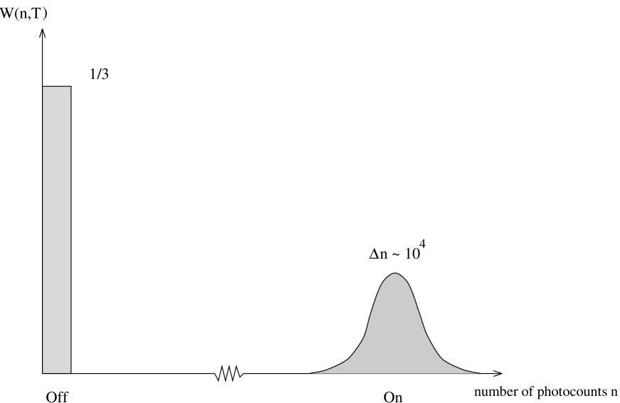


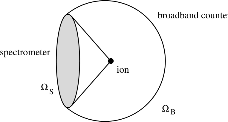


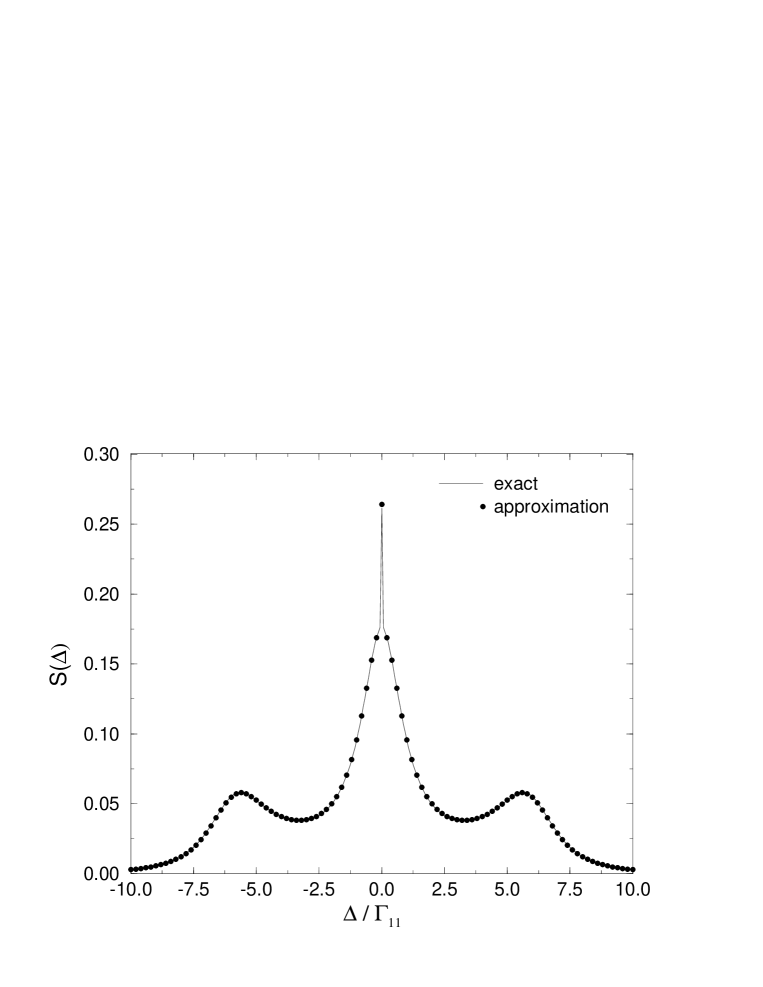

.

.

