Classical statistical distributions can violate Bell-type inequalities

Abstract

We investigate two-particle phase-space distributions in classical mechanics constructed to be the analogs of quantum mechanical angular momentum eigenstates. We obtain the phase-space averages of specific observables related to the projection of the particles’ angular momentum along axes with different orientations, and show that the ensuing correlation function violates Bell’s inequality. The key to the violation resides in choosing observables impeding the realization of the joint measurements whose existence is required in the derivation of the inequalities. This situation can have statistical (detection related) or dynamical (interaction related) underpinnings, but non-locality does not play any role.

I Introduction

Bell’s theorem was originally introduced bell1964 to examine quantitatively the consequences of postulating hidden variable distributions on the incompleteness of quantum mechanics put forward by Einstein, Podolsky and Rosen EPR (EPR). The core of the theorem takes the form of inequalities involving average values of two observables each related to one of the two particles. Bell showed that these inequalities must be satisfied by any theory containing local variables aiming to complete quantum mechanics in the EPR sense. The assumptions leading to Bell’s theorem imply the existence of a joint probability distribution accounting for the simultaneous existence of incompatible quantum observables fine82 ; cabello96 . Local models forbidding the existence of these joint distributions are therefore not bound by Bell’s theorem. Indeed local models violating Bell-type inequalities have already been proposed beltrametti ; orlov ; christian , but these models are mathematical and abstract. In this work, we show that the familiar statistical distributions of classical mechanics may lead to a violation of the relevant Bell-type inequalities. Our main ingredients will consist first in choosing specific classical phase-space ensembles for 2 particles (distributions constructed to be the classical analogs of the quantum-mechanical angular momenta eigenstates), and then in choosing detectors impeding the existence of the joint probability distribution. We will consider two types of settings involving angular momentum measurements, each setting being closely related to a well-known quantum mechanical context. The first setting will consist in a classical version of the detection loophole percival : the relevant Bell inequalities will be seen to be violated when the sampling is done on a sub-ensemble, defined by the type of detected events, leading to averages computed on a partial region of phase-space over which the joint probability distribution cannot be defined. Hence the violation has a statistical underpinning – we will show there is no violation if the averages are taken on the entire phase-space. The second setting will reveal a genuine violation of the Bell inequalities due to dynamical reasons: by including in the detection process a local probabilistic interaction between the measured particle and the detector inducing a random perturbation that blurs the particles’ phase-space positions, the derivation of Bell’s theorem is effectively blocked, as only correlations between ensembles corresponding to a fixed setting of the detectors can be made. This example can be seen as a classical version of the quantum measurement of non-commuting observables.

II Classical ensembles

We first introduce the classical analogs of the quantum mechanical angular-momentum eigenstates to be employed below. The classical distributions of particles can be considered either in phase-space or in configuration space; equivalently, one can also consider the distribution of the angular momenta on the angular momentum sphere. Let us first take a single classical particle and assume the modulus $J$ of its angular momentum is fixed. The value of $\mathbf{J}$ then depends on the position of the particle in the phase-space defined by $\Omega=\{\theta,\phi,p_{\theta},p_{\phi}\},$ where $\theta$ and $\phi$ refer to the polar and azimuthal angles in spherical coordinates and $p_{\theta}$ and $p_{\phi}$ are the conjugate canonical momenta. Let $\rho_{z}(\Omega)$ be the distribution in phase-space given by

$$\rho_{z_{0}}(\theta,\phi,p_{\theta},p_{\phi})=N\delta(J_{{}_{z}}(\Omega)-J_{z_{0}})\delta(J^{2}(\Omega)-J_{0}^{2}).$$ (1)

$\rho_{z_{0}}$ defines a distribution in which every particle has an angular momentum with the same magnitude, namely $J_{0}$, and the same projection on the $z$ axis $J_{z_{0}}$. Hence $\rho_{z_{0}}$ can be considered as a classical analog of the quantum mechanical density matrix $\left|jm\right\rangle\left\langle jm\right|$ since just like a quantum measurement of the magnitude $j$ and of the $z$ axis projection $m$ of the angular momentum in such a state will invariably yield the eigenvalues of the operators $\hat{J}^{2}$ and $\hat{J}_{z}$, the classical measurement of these quantities when the phase-space distribution is known to be $\rho_{z}$ will give $J_{0}^{2}$ and $J_{z_{0}}$ (see Appendix A). Eq. (1) can be integrated over the conjugate momenta to yield the configuration space distribution

$$\rho(\theta,\phi)=N\left[\sin(\theta)\sqrt{J_{0}^{2}-J_{z_{0}}^{2}/\sin^{2}(\theta)}\right]^{-1}$$ (2)

where we have used the defining relations $J_{{}_{z}}(\Omega)=p_{\phi}$ and $J^{2}(\Omega)=p_{\theta}^{2}+p_{\phi}^{2}/\sin^{2}\theta$. Further integrating over $\theta$ and $\phi$ and requiring the phase-space integration of $\rho$ to be unity allows to set the normalization constant $N=J_{0}/2\pi^{2}$.

There is of course nothing special about the $z$ axis and we can define a distribution by fixing the projection $J_{a}$ of the angular momentum on an arbitrary axis $a$ to be constant (in this paper we will take all the axes to lie in the $zy$ plane). Computing the distribution $\rho_{a_{0}}=\delta(J_{a}-J_{a_{0}})\delta(J-J_{0}^{2})$ is tantamount to rotating the coordinates towards the $a$ axis in Eq. (2). Fig. 1 shows examples of configuration space particle distributions and gives for one plot the corresponding quantum mechanical angular-momentum eigenstate (the similarity is not accidental, as Eq. (2) is essentially the amplitude of the spherical harmonic in the semiclassical regime, see Appendix A). We can also determine the average projection $J_{a}$ on the $a$ axis for a distribution of the type (2) corresponding to a well defined value of $J_{z}$:

$$\left\langle J_{a}\right\rangle_{J_{z_{0}}}=\int p_{\phi}\cos\theta_{a}\delta(J_{{}_{z}}(\Omega)-J_{z_{0}})d\Omega=J_{z_{0}}\cos\theta_{a},$$ (3)

where $\theta_{a}$ is the angle $(\widehat{z,a})$ and the projection of the component of $J_{a}$ on the $y$ axis vanishes given the axial symmetry of the distribution.

The original derivation of the inequalities by Bell bell1964 involved the measurement of the angular momentum of 2 spin-$1/2$ particles along different axes. Here we will consider the fragmentation of an initial particle with a total angular momentum $\mathbf{J}_{T}=0$ into 2 particles carrying angular momenta $\mathbf{J}_{1}$ and $\mathbf{J}_{2}$ (we will assume to be dealing with orbital angular momenta). Conservation of the total angular momentum imposes $\mathbf{J}_{1}=-\mathbf{J}_{2}$ and $J_{1}=J_{2}\equiv J.$ Quantum mechanically, this situation would correspond to the system being in the singlet state arising from the composition of the angular momenta ($j_{T}=0$, $m_{1}=-m_{2}$). Classically the system is represented by the 2-particle phase space distribution

$$\rho(\Omega_{1},\Omega_{2})=N\delta(\mathbf{J}_{1}+\mathbf{J}_{2}),$$ (4)

where $N$ is again a normalization constant. On the angular momentum sphere the distribution (4) corresponds to $\mathbf{J}_{1}$ and $\mathbf{J}_{2}$ being uniformly distributed on the sphere but pointing in opposite directions. This distribution will now be employed for determining averages of observables related to the angular momenta of the two particles.

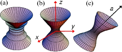
Figure 1: Normalized angular distribution for a single particle in configuration space. (a) Quantum distribution (spherical harmonic $|Y_{JM}(\theta,\phi)|^{2}$). (b) Classical distribution $\rho_{z_{0}}(\theta,\phi)$ of Eq. (2). (c) Classical distribution $\rho_{a_{0}}$ corresponding to a fixed value of $J_{a}$ (here $\theta_{a}=\pi/4$). The angular momentum and the projection on the $z$ [(a)-(b)] or $a$ [(c)] axis is the same for the 3 plots ($J/\eta=40$, with $\eta=\hbar$, and $M/J=5/8$).

III Statistical violation of the Bell inequalities

Let us assume two types of detectors yielding outcomes related to the angular momenta of the particles. The first type gives a ’sharp’ (S) measurement of $J_{1a}$ only if $J_{1a}$ is an integer multiple of some elementary gauge $\eta$, and gives $0$ elsewhere. This detection can be represented by the phase-space quantity

$$S_{a}(\Omega_{1})=J_{1a}(\Omega_{1})\textrm{ if }\Omega_{1}\in\Omega_{1k},\\ S_{a}(\Omega_{1})=0\textrm{ elsewhere,}$$ (5)

where $\Omega_{1k}$ are the parts of phase space where $J_{1a}=k\eta$ compatible with a detection (see Fig. 2(a)). The second detector gives a ’direct’ (D) measurement of $J_{2b}$ (the projection of $\mathbf{J}_{2}$ on an axis $b$). The corresponding phase-space function is

$$D_{b}(\Omega_{2})=\mathbf{J}_{2}\cdot\mathbf{b.}$$ (6)

In classical mechanics there is no natural unit for quantities having the dimension of an action, so $J$ and $\eta$ can be expressed in terms of arbitrary units, and any physical result will depend only on the ratio $J/\eta$. We will assume for definiteness that $\eta$ is chosen so that the extremal values $\pm J$ can be reached. $J/\eta$ must hence be either an integer or a half-integer, the extremal values in dimensionless units being given by $\pm L\equiv\pm J/\eta$. For example if $\eta=2J$, the measurement can only yield the extremal values $L=\pm 1/2$ ($\eta=J$ allows to measure $\pm L=\pm 1$ and 0, $\eta=2J/3$ allows $\pm L=\pm 3/2$ and $\pm(L-1)=\pm 1/2$ etc.). Note that the particle label $1$ or $2$ can be attached to the detectors: indeed, we will call ’1’ the particle detected by S and ’2’ the particle detected by D.

The classical average $E(a,b)=\left\langle S_{a}D_{b}\right\rangle$ for joint measurements over the statistical distribution $\rho$ can be computed from

$$E(a,b)=\int S_{a}(\Omega_{1})D_{b}(\Omega_{2})\rho(\Omega_{1},\Omega_{2})d\Omega_{1}d\Omega_{2}$$ (7)

with Eqs. (4), (5) and (6). Given the characteristics (5) of the S detection, Eq. (7) is actually a discrete sum over the parts of phase-space $\Omega_{1k}$ leading to the detection of $k\eta$; this can be written by including a delta function under the integral. Eq. (4) imposes $\theta_{2}=\pi-\theta_{1}$ and $\phi_{2}=\pi+\phi_{1},$ and Eq. (7) becomes

$$E(a,b)=\frac{1}{2}\sum_{k=-L}^{k=L}\int\left[L\cos\theta_{1}\right]\delta\left(L\cos\theta_{1}-k\right)\left[-L\cos\theta_{1}\cos(\theta_{b}-\theta_{a})\right]\sin\theta_{1}d\theta_{1},$$ (8)

where we have chosen the $z$ axis to coincide with $a$ to take advantage of the axial symmetry imposed by $S_{a}$ (here the limiting procedure in the delta function is understated). The $\frac{1}{2}$ prefactor is the only nontrivial normalisation factor (coming from the integration over $\theta_{1}$). We obtain the average as

$$E(a,b)=-\frac{1}{6}(L+1)(2L+1)\cos(\theta_{b}-\theta_{a}),$$ (9)

which as expected depends solely on the ratio $J/\eta\equiv L$.

The correlation function employed in Bell’s inequality can be obtained in the standard (or CHSH) form CHSH69 ; bell2 . We choose 4 axes $a$, $b\mathbf{,}$ $a^{\prime}$, $b^{\prime}$ (we can assume an S detector is placed along ${a}$ and $a^{\prime}$, and a D detector along ${b}$ and ${b}^{\prime}$) and determine the average values for each of the 4 possible combinations involving an S and a D detector. The correlation function $C$ relating the average values obtained for different orientation of the detectors’ axes is

$$C(a,b,a^{\prime},b^{\prime})=\left(\left|E(a,b)-E(a,b^{\prime})\right|+\left|E(a^{\prime},b)+E(a^{\prime},b^{\prime})\right|\right)(L)^{-2}$$ (10)

where we have divided by $L^{2}$ to obtain the CHSH function in the standard form characterized by values bounded by $\pm 1$. Here the detected values obey the conditions $\left|S/L\right|\leq 1$ and $\left|D/L\right|\leq 1$, so that the usual derivation of the Bell inequalities would lead to

$$C(a,b,a^{\prime},b^{\prime})\leq 2.$$ (11)

By replacing Eq. (9) in Eq. (10), it can be seen that for $L=\frac{1}{2}$, $1$ and $\frac{3}{2}$, there are several choices of the axes that lead to $C(a,b,a^{\prime},b^{\prime})>2$. The maximal value of the correlation function corresponds to $C(0,\frac{\pi}{4},\frac{\pi}{2},\frac{3\pi}{4})=4\sqrt{2}$ and $2\sqrt{2}$ for $L=\frac{1}{2}\$and $1$ respectively .

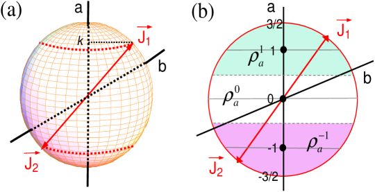
Figure 2: Setups for the first (a) and second (b) examples investigated in this work. In (a) an S detector is placed along the $a$ axis and a D detector along $b$. The angular momenta, originally distributed on the sphere, are constrained to move on the rings (red dotted) corresponding to fixed values of the projection on $a$. (b) shows the $(\widehat{z,y})$ plane of the angular momentum sphere for the $L=1$ case (hence $J=3/2$); the 3 zones correspond to the projections of the spherical zones $\rho_{a}^{-1}$, $\rho_{a}^{0}$ and $\rho_{a}^{+1}$. If $J_{a}$ is measured, the presence of $\mathbf{J}$ in one of these zones yields the outcomes $J_{a}=-1,0,1$ with unit probability. If $J_{b}$ is measured and $\mathbf{J}\in\rho_{a}^{k}$ any of the outcomes $J_{b}=-1,0,1$ can be obtained with probabilities depending on the distribution $\rho_{a}^{k}$.

The violation of the Bell inequality is due to the fact that we are only including in the statistics the measurements for which both the S and the D detectors click. But when an S-measurement is made along the two different orientations $a$ and $a^{\prime}$ that enter the correlation function, different and mutually exclusive parts of phase-space are selected, so that the different events

$$\{S_{1a},D_{2b}\},\{S_{1a^{\prime}},D_{2b}\},\{S_{1a},D_{2b^{\prime}}\},\textrm{ and }\{S_{1a^{\prime}},D_{2b^{\prime}}\}$$ (12)

are not supported by a common phase-space distribution. As a consequence the quantity

$$\int S_{a}(\Omega_{1})D_{b}(\Omega_{2})S_{a^{\prime}}(\Omega_{1})D_{b^{\prime}}(\Omega_{2})\rho(\Omega_{1,}\Omega_{2})d\Omega_{1}d\Omega_{2}$$ (13)

describing the average of simultaneous measurements along the 4 axes becomes undefined. However, as we mentioned above, the existence of the joint probability distribution in the integrand of Eq. (13), or equivalently accardi , of a common distribution for the events (12) is a necessary ingredient in the derivation of Bell’s theorem, thereby explaining the violation of the inequalities. It is noteworthy that if one includes the entire phase-space in the average (7) instead of the parts of phase-space corresponding to the double-click events, then Eq. (13) becomes well-defined. It can then be shown that $E(a,b)$ and $C(a,b,a^{\prime},b^{\prime})$ should be multiplied by the fraction of phase-space yielding the double click measurements: as a result Bell’s inequality would not be violated. From the standpoint of classical mechanics, the objection regarding the necessity of including the entire phase-space makes sense, since one can envisage in principle a particle analyzer able to detect the particles that have not been included in the double-click statistics. The quantum analog of this problem is the well-known detection loophole, pending on the experimental tests of Bell’s inequalities percival ; santos .

IV Dynamically induced violation of the Bell inequalities

Our second setting goes further into the violation of Bell’s inequalities by postulating a model involving a local probabilistic interaction during the measurement between the detector and the particle being measured: we then obtain a violation of the inequality for the entire ensemble of particles. Let us take two identical detectors $T_{1}$ and $T_{2}$ that give as only output the integer or half-integer values $k=L,L-1,...-L$ of the projection $J_{1a}$ and $J_{2b}$ of the angular momenta of the particles. We choose here $L=J/\eta-1/2$, from which it follows that the maximal readout $L$ is smaller than $J$; for notational simplicity we put $\eta=1$ (so $J$, rather than $J/\eta$ takes integer or half integer values). We further assume that there is an interaction between $T_{1}$ and particle $1$ (and between $T_{2}$ and particle $2$) affecting the angular momentum of the particle so that the transition $J_{1a}\rightarrow k$ is a physical process due to the measurement.

We impose the following constraints on this process (which only involves a single particle and its measuring apparatus, hence we drop the indices labeling the particles).

1. There are distributions $\rho_{a}^{k}$ such that if $\mathbf{J}\in\rho_{a}^{k}$

   $$P_{k^{\prime}}^{T_{a}}(\mathbf{J}\in\rho_{a}^{k})=\delta_{kk^{\prime}}.$$ (14)

   This means that if $T_{a}$ is measured and we obtain $k$ then we know that previous to the measurement $\mathbf{J}\in\rho_{a}^{k}$ with unit probability.

2. Let $\left\langle J_{b}\right\rangle_{\rho_{a}^{k}}$ be the phase-space average of $J_{b}$ over the distribution $\rho_{a}^{k}$, where the directions $b$ and $a$ are assumed to be different. If $T_{b}$ is measured and $\mathbf{J}\in\rho_{a}^{k}$, any outcome $k^{\prime}$ can be obtained with a non-vanishing probability $P_{k^{\prime}}^{T_{b}}(\mathbf{J}\in\rho_{a}^{k}).$ Our main assumption is that averaging over $T_{b}$ gives the phase-space average of $J_{b}$, i.e. the interaction vanishes on average. This constraint takes the form

   $$\left\langle T_{b}\right\rangle_{\rho_{a}^{k}}=\sum_{k^{\prime}=-L}^{L}k^{\prime}P_{k^{\prime}}^{T_{b}}(\mathbf{J}\in\rho_{a}^{k})=\left\langle J_{b}\right\rangle_{\rho_{a}^{k}}.$$ (15)

   Eq. (15) also holds if $b=a$ but then only $P_{k}^{T_{a}}=1$ is non-vanishing hence

   $$\left\langle T_{a}\right\rangle_{\rho_{a}^{k}}=\left\langle J_{a}\right\rangle_{\rho_{a}^{k}}=k.$$ (16)

We will not be interested here in putting forward specific models of the interaction yielding such probabilities; it will suffice for our purpose that a set of numbers $P_{k}$ verifying Eq. (15) and obeying $\sum_{k}P_{k}=1$ can be obtained. We need to specify however the distributions obeying Eq. (14). It is convenient to specify $\rho_{a}^{k}$ in terms of the distribution of $\mathbf{J}$ on the angular momentum sphere: it can then easily be seen that Eq. (16) is realized if $\rho_{a}^{k}$ is taken to be the ring centered on the $a$ axis and bounded by $k-1/2<J_{a}<k+1/2$ (see Fig. 2(b)). Then a measurement of $T_{a}$ will yield the outcome $k$ with unit probability:

$$T_{a}=k\textrm{ if }k-1/2<J_{a}<k+1/2.$$ (17)

One can of course envisage a distribution $\rho$ obtained by combining the elementary ensembles $\rho_{a}^{k}$. In particular the uniform distribution on the sphere $\rho_{\Sigma}$ is the sum of the $2L+1$ spherical rings $\rho_{a}^{k}$,

$$\rho_{\Sigma}=\sum_{k}\frac{\rho_{a}^{k}}{2L+1}$$ (18)

and therefore if $T_{a}$ is measured the probability of finding a given value $k$ is $P=$$1/(2L+1)$. Inversely the obtention of the given outcome $k$ is correlated with $\mathbf{J}\in\rho_{a}^{k}$ previous to the measurement. With $\rho_{a}^{k}$ defined in this way [Eq. (17)], $\left\langle J_{b}\right\rangle_{\rho_{a}^{k}}$ is computed straightforwardly and Eq. (15) becomes

$$\left\langle T_{b}\right\rangle_{\rho_{a}^{k}}=k\cos(\theta_{b}-\theta_{a});$$ (19)

we see again that for correlations involving averages, the knowledge of the individual probabilities $P_{k}^{T_{b}}$ is not necessary. Note however that for the particular case $J=1$ (i.e., $L=1/2$) the constraints (15)-(17) as well as the normalization of the probabilities impose the values of the $P_{k}^{T_{b}}$ irrespective of any precise physical process: indeed $k$ can only take the values $\pm-1/2$ from which it follows that

$$P_{\pm}^{T_{b}}=\frac{1}{2}\pm\left\langle J_{a}\right\rangle_{\rho_{a}^{k}}=\frac{1}{2}\pm k\cos\left(\theta_{b}-\theta_{a}\right).$$ (20)

Let us now go back to the 2-particle problem, assuming the initial phase-space density $\rho$ given by Eq. (4). The expectation value $E(a,b)=\left\langle T_{1a}T_{2b}\right\rangle$ is computed from the general formula

$$E(a,b)=\sum_{k,k^{\prime}=-L}^{L}kk^{\prime}P(T_{2b}=k^{\prime}\cap T_{1a}=k)$$ (21)

where $k$ and $k^{\prime}$ run on the possible outcomes. The probabilities of obtaining $T_{1a}=k$ and $T_{2b}=k^{\prime}$ are obtained in the following way. Using

$$P(T_{2b}=k^{\prime}\cap T_{1a}=k)=P(T_{1a}=k)P(T_{2b}=k^{\prime}|T_{1a}=k)$$ (22)

we first determine $P(T_{1a}=k)$ by remarking that the initial distribution $\rho$ corresponds to $\mathbf{J}_{1}$ being uniformly distributed on the sphere. According to the results of the preceding paragraph, with the sphere being cut into $2L+1$ equiprobable zones $\rho_{a}^{k}$ [see Eq. (18)], we have $P(T_{1a}=k)=1/(2L+1)$. We also know that an outcome $T_{1a}=k$ corresponds to $\mathbf{J}_{1}\in\rho_{a}^{k}$ [Eq. (14)]. From the conservation of the total angular momentum, we infer that particle 2 must lie in the zone $\rho_{a}^{-k}$ defined by $k-1/2<-J_{2a}<k+1/2$ [Eq. (17)]; indeed if $T_{2a}$ were to be measured we would be assured of finding $T_{2a}=-T_{1a}=-k$. Hence the conditional probability appearing in Eq. (22) is given by

$$P(T_{2b}=k^{\prime}|T_{1a}=k)=P_{k^{\prime}}^{T_{b}}(\mathbf{J}_{2}\in\rho_{a}^{-k})$$ (23)

where $P_{k^{\prime}}^{T_{b}}$ was defined in Eq. (15). The sum over $k^{\prime}$ in Eq. (21) thus verifies Eq. (15) and having in mind Eq. (19), the expectation value becomes

$$E(a,b)=\sum_{k=-L}^{L}\frac{-k^{2}}{2L+1}\cos(\theta_{b}-\theta_{a})=\frac{-L(L+1)}{3}\cos(\theta_{b}-\theta_{a}).$$ (24)

The correlation function is again given by Eq. (10), since the maximum value detected by a T measurement is $L,$ not $J$. The result given by Eq. (24) is familiar from quantum mechanics – it violates Bell’s inequality for $L=1/2$ with a maximal violation for $C(0,\frac{\pi}{4},\frac{\pi}{2},\frac{3\pi}{4})=2\sqrt{2}$. As noted for the single particle case, the derivation of $E(a,b)$ does not depend in any way on the individual values of the probabilities $P_{k^{\prime}}^{T_{b}}$ but only on the condition (15) regarding the particle-measurement interaction. Note that by Bayes’ theorem, it is of course equivalent to compute $P(T_{2b}=k^{\prime}\cap T_{1a}=k)$ from $P(T_{2b}=k^{\prime})P(T_{1a}=k|T_{2b}=k^{\prime})$, ie by assuming that $T_{2b}=k^{\prime}$ is known first.

The violation of the Bell inequalities is due to the conjunction of two ingredients. The first, represented by the constraints (14)-(16), is relative to a single particle and its interaction with the measurement apparatus. The second is the conservation of the angular momentum on average. Interestingly the first ingredient is the one that contradicts the assumptions made in the derivation of Bell’s theorem. The reason is that Eqs. (14)-(16) are incompatible with the introduction of elementary probability functions $p_{k}^{T_{b}}(\Omega)$ such that

$$P_{k^{\prime}}^{T_{b}}(\mathbf{J}\in\rho_{a}^{k})=\int p_{k^{\prime}}^{T_{b}}(\Omega)\rho_{a}^{k}(\Omega)d\Omega;$$ (25)

indeed, such probability functions would need to depend on the ensemble, giving rise to functions of the type $p_{k}^{T_{b}}(\Omega;\rho_{a}^{k})$. This is shown for the case $L=1/2$ in Appendix B. With this point in mind, one can expand Eq. (21) (with Eqs. (22), (18) and (23)) as

$$E(a,b)=\int\sum_{k}kp_{k}^{T_{a}}(\Omega_{1};\rho_{\Sigma})\rho_{\Sigma}(\Omega_{1})d\Omega_{1}\int B(\Omega_{2},k)\rho_{a}^{-k}(\Omega_{2})d\Omega_{2}$$ (26)

with

$$B(\Omega_{2},k)\equiv\sum_{k^{\prime}}k^{\prime}p_{k^{\prime}}^{T_{b}}(\Omega_{2};\rho_{a}^{-k}).$$ (27)

The dependence of $B$ on $k$ is the crucial property allowing to violate Bell’s inequality (whereas the dependence of $\rho(\Omega_{2})$ on $k$ in Eq. (26) by itself can be absorbed in the initial correlation $\delta(\mathbf{J}_{1}+\mathbf{J}_{2})$ provided $k=k(\Omega_{1})$). The dependence of $B$ on $k$ has nothing to do with non-locality or action at a distance. It is a simple consequence of the logical inference characterizing the conditional probability (22) given the characteristics of the single particle interaction with the measuring apparatus, namely the fact that the model allows only specific types of correlations: in the single particle problem one can only correlate a given outcome with a specific distribution – this happens when the distribution is symmetric relative to the detector’s axis [Eq. (14)]; in the two particle problem the single particle property just mentioned makes only possible the correlation of $\mathbf{J}_{2}$ as a function of $\mathbf{J}_{1}$ in terms of the ensembles to which they belong, not in terms of their individual positions. This is consistent with the fact that the knowledge of the individual position of $\mathbf{J}$ is meaningless to compute the observed probabilities, as even the elementary probabilities must depend on the ensemble to which the angular momentum belongs.

Note finally that would $B$ not depend on $k$ (and the elementary probabilities on the ensembles), Eq. (26) would turn into

$$E^{BT}(a,b)=\int A(\Omega_{1})B(\Omega_{2})\rho(\Omega_{1},\Omega_{2})d\Omega_{1}d\Omega_{2}$$ (28)

where

$$A(\Omega_{1})\equiv\sum_{k}kp_{k}^{T_{a}}(\Omega_{1})\textrm{ \ \ }B(\Omega_{2})\equiv\sum_{k^{\prime}}k^{\prime}p_{k^{\prime}}^{T_{b}}(\Omega_{2}),$$ (29)

thereby yielding the familiar form taken by the expectation value in the derivation of Bell’s theorem. In the deterministic case considered by Bell bell2 the functions $p_{k}^{T_{a}}$ and $p_{k^{\prime}}^{T_{b}}$ are either $0$ or $1$ depending on the individual position of $\mathbf{J}_{1}$ (resp. $\mathbf{J}_{2}$). This implies that $k=k(\Omega_{1})$, ie a given outcome depends on the position of $\mathbf{J}_{1}$ on the angular momentum sphere, and $\rho_{a}^{-k}(\Omega_{2})=\rho(\Omega_{2}|\mathbf{J}_{1})$ does not depend on $k$ or $a$ but on $\mathbf{J}_{1}=-\mathbf{J}_{2}$ (hence the inclusion of the term $\delta(\mathbf{J}_{1}+\mathbf{J}_{2})$ in the definition of $\rho(\Omega_{1},\Omega_{2})$). Conversely one may assume $\rho(\Omega_{2}|k)=\rho(\Omega_{2}|\Omega_{1})$ in Eq. (26) with $p_{a}^{k}(\Omega_{1})$ and $p_{b}^{k^{\prime}}(\Omega_{2})$ being probability functions different from $0$ or $1$; then $A$ and $B$ defined in Eq. (29) are not the observed outcomes but their averages, and $E^{BT}(a,b)$ is the expectation corresponding to the stochastic case considered by Bell. Bell’s stochastic case correlates the individual positions of $\mathbf{J}_{1}$ and $\mathbf{J}_{2}\$to possible outcomes with definite probabilities. In the present model the random interaction forbids to make the correspondence between a given position of the angular momenta and a definite outcome; instead the correspondence is between a definite outcome and a given ensemble describing the positions of the angular momenta compatible with the outcome (of course if the former correspondence is satisfied, so is the latter, but the converse is not true). In the latter case, the structure of the expectation value (26) does not allow to define a term of the type given by Eq. (13) whereby a single distribution can account for several simultaneous joint measurements. It appears indeed that the ensemble dependency exhibited by the present model is a necessary feature in order to produce non-commuting measurements matz-p . In this sense the present model can be seen as a classical analogue of the quantum measurement of two non-commuting observables (such as $J_{1a}$ and $J_{1a^{\prime}}$) applied to correlations between two particles as originally considered by EPR EPR .

V Conclusion

The present results show that averages obtained with 2-particle classical distributions constructed to be the analogs of quantum mechanical eigenstates can violate Bell’s inequalities. The violation does not involve nonlocality but statistical or dynamical processes that impede the existence of joint probability distributions or the correlation between individual values of the variables as required by Bell’s theorem. Possible implications on the role of the Bell-CHSH argument as a marker of quantum nonlocality, which has recently been criticized unruh , will be examined elsewhere matz-p .

Appendix A

The scheme we are employing to contruct the classical distributions rests on the well-known analogy between the classical Poisson brackets and the quantum commutation relations in the density matrix formalism. Let $\hat{G}$ be an operator and $\left|\psi_{g}\right\rangle$ an eigenstate with eigenvalue $g.$ Then the pure-state density matrix $\hat{\rho}_{g}\equiv\left|\psi_{g}\right\rangle\left\langle\psi_{g}\right|$ verifies $[\hat{\rho}_{g},\hat{G}]=0$ and $\hat{G}\hat{\rho}_{g}=g\hat{\rho}_{g}$. In classical mechanics the Poisson bracket of two phase space quantities $u(q,p)$ and $v(q,p)$ is a canonical invariant defined by goldstein

$$\{u,v\}=\frac{\partial u}{\partial q}\frac{\partial v}{\partial p}-\frac{\partial u}{\partial p}\frac{\partial v}{\partial q}.$$ (30)

Let $\rho(q,p)$ be the phase-space distribution and $G(q,p)$ be a function such that $\{\rho,G\}=0.$ This means that $\rho$ is invariant relative to the canonical tranformation generated by $G$, ie

$$\{\rho,G\}\delta Q_{G}=\delta\rho=0,$$ (31)

where $Q_{G}$ is canonically conjugate to $G$, which is a constant of the motion. Then every point of the distribution $\rho$ will be characterized by the constant value taken by $G$, denoted $g$. If this is the only constraint imposed on the distribution, $\rho(q,p)$ will take the form (up to a normalization constant)

$$\rho(q,p)=\delta(G(q,p)-g).$$ (32)

In configuration space, the distribution $\rho(q)$ is obtained by integrating over the values of the momentum compatible with a given $q,$

$$\rho(q)=\int\rho(q,p)dp=\int\frac{\delta(p-p_{i})}{\left.\frac{\partial G}{\partial p}\right|_{p_{i}}}dp$$ (33)

where $p_{i}$ is the root (assumed to be unique, else a sum is in order) of the argument of the delta function. Integrating yields

$$\rho(q)=\left.\frac{\partial p}{\partial G}\right|_{p_{i}}=\left.\frac{\partial^{2}S}{\partial q\partial G}\right|_{p_{i}}$$ (34)

where $S(q,G)$ is the classical action. The configuration space density is therefore the amplitude of the quantum density matrix element $\left\langle q\right|\hat{\rho}_{g}\left|q\right\rangle$ in the semiclassical approximation.

Appendix B

We show that the detection model for a single particle given in Sec. 4 is inconsistent with probability functions defined by Eq. (25) in the $L=1/2$ case (the one violating the Bell inequalities). Take Eq. (25) with $a=b$ and $k,k^{\prime}=+1/2$,

$$P_{+}^{T_{b}}(\mathbf{J}\in\rho_{b}^{+})=\int p_{+}^{T_{b}}(\Omega)\rho_{b}^{+}(\Omega)d\Omega=1.$$ (35)

Particularizing the general formula (17) to the case $L=1/2$, $\rho_{b}^{+}$ is the positive hemisphere of the unit sphere (since $J=1$) centered on the $b$ axis. The result on the right handside follows from Eq. (20). Eq. (35) implies that $p_{+}^{T_{b}}(\Omega)=1$ for $\mathbf{J}\in\rho_{b}^{+}$ and consequently $p_{-}^{T_{b}}(\Omega)=0$. Conversely since $P_{+}^{T_{b}}(\mathbf{J}\in\rho_{b}^{-})=0$, we must have $p_{+}^{T_{b}}(\Omega)=0$ and $p_{-}^{T_{b}}(\Omega)=1$ when $\mathbf{J}\in\rho_{b}^{-}$. Now assume that the distribution is instead $\rho_{a}^{+}$ with $a$ different from the $b$ axis. Then according to our model [Eq. (20)] we should have

$$P_{+}^{T_{b}}(\mathbf{J}\in\rho_{a}^{+})=\int p_{+}^{T_{b}}(\Omega)\rho_{a}^{+}(\Omega)d\Omega=\cos^{2}\frac{\theta_{b}-\theta_{a}}{2}.$$ (36)

Noting that $\rho_{a}^{+},$ the positive hemisphere centered on $a$, is actually composed of two parts, $\rho_{a}^{+}\cap\rho_{b}^{+}$ and $\rho_{a}^{+}\cap\rho_{b}^{-}$ we can write

$$P_{+}^{T_{b}}(\mathbf{J}\in\rho_{a}^{+})=\int_{\rho_{a}^{+}\cap\rho_{b}^{+}}p_{+}^{T_{b}}(\Omega)\rho_{a}^{+}(\Omega)d\Omega+\int_{\rho_{a}^{+}\cap\rho_{b}^{-}}p_{+}^{T_{b}}(\Omega)\rho_{a}^{+}(\Omega)d\Omega.$$ (37)

But we have seen that $p_{+}^{T_{b}}=1$ for $\mathbf{J}\in\rho_{b}^{+}$ and $p_{+}^{T_{b}}(\Omega)=0$ for $\mathbf{J}\in\rho_{b}^{-}$, hence

$$P_{+}^{T_{b}}(\mathbf{J}\in\rho_{a}^{+})=\int_{\rho_{a}^{+}\cap\rho_{b}^{+}}\rho_{a}^{+}(\Omega)d\Omega=1-\frac{\theta_{b}-\theta_{a}}{\pi},$$ (38)

which contradicts Eq. (36). Hence probability functions obeying Eq. (25) do not exist, and Eq. (25) should be replaced by

$$P_{k^{\prime}}^{T_{b}}(\mathbf{J}\in\rho_{a}^{k})=\int p_{k^{\prime}}^{T_{b}}(\Omega;\rho_{a}^{k})\rho_{a}^{k}(\Omega)d\Omega$$ (39)

where the notation $p_{k^{\prime}}^{T_{b}}(\Omega;\rho_{a}^{k})$ denotes the dependence of the elementary probabilities on the distribution. Note also that Eq. (25) does hold if one drops the requirement that $p_{k^{\prime}}^{T_{b}}(\Omega)$ should represent an elementary probability: for example the functions $p_{+}^{T_{b}}(\Omega)=J_{b}+1/2$ or $p_{+}^{T_{b}}(\Omega)=2J_{b}H(J_{b})\$fulfill Eq. (36) without depending on the distribution, though none of these functions is contained in the interval $[0,1]$ and are thus not probability functions. We stress that these features, which put strong constraints on the type of admissible physical models that one could envisage, are relevant to a single particle and its interaction with the measurement apparatus.

References

- (1) J. S. Bell 1964 Physics 1, 195.
- (2) A. Einstein, B. Podolsky and N. Rosen 1935 Phys. Rev. 47 777.
- (3) A. Fine 1982 J. Math. Phys. 23 1306.
- (4) A. Cabello and G. Garcia-Alcaine 1997, J. Phys. A: Math. Gen. 30 725.
- (5) E G Beltrametti and S Bugajski 1996, J. Phys. A: Math. Gen. 29 247.
- (6) Y. F. Orlov 2002 Phys. Rev. A 65, 042106.
- (7) J. Christian 2007 E-print arXiv:quant-ph/0707.1333 .
- (8) R. M. Basoalto and I. C. Percival 2003 J. Phys. A: Math. Gen. 36 7411, and Refs therein.
- (9) J. F. Clauser, M. A. Horne, A. Shimony, and R. A. Holt 1969, Phys. Rev. Lett. 28, 880.
- (10) J. S. Bell 2004, Speakable and unspeakable in quantum mechanics, Cambridge Univ. Press, ch. 4.
- (11) L. Accardi and M. Regoli 2000 E-print arXiv:quant-ph/0007005.
- (12) A. Matzkin, in prep.
- (13) E. Santos 1992 Phys. Rev. A 46, 3646 (1992).
- (14) W. Unruh 2006 Int. Jour. Qu. Inf. 4, 209.
- (15) H. Goldstein 1980, Classical Mechanics, Addison-Wesley.