Instantaneous processing of ”slow light”: amplitude-duration control, storage, and splitting

Abstract

Nonadiabatic change of the control field or of the low-frequency coherence allows for an almost instantaneous change of the signal field propagating in a thick resonant absorber where electromagnetically induced transparency is realized. This finding is applied for the storage and retrieval of the signal, for the creation of a signal copy and separation of this copy from the original pulse without its destruction.

A seminal idea of storage and retrieval of light pulses (SRLP) using a medium with electromagnetically induced transparency (EIT) was proposed in Ref. Lukin2000 by Fleischhauer and Lukin. Shortly after the proposal, SRLP was experimentally demonstrated in ultracold Na Liu , in hot Rb vapor Phillips , and in a solid (Pr:YSO) Turukhin . Later, SRLP received much attention in the framework of quantum computing and quantum memory (see, for example, Ref. Kuzmich ). The core idea of such a storage is the dark-state polariton Lukin2000 . This is a particular superposition of the pulse amplitude and the atomic coherence created in a two-quantum process by signal and control fields. The signal pulse drives the transition from the populated ground state $\left|g\right\rangle$ to an excited state $\left|e\right\rangle$, and the cw control field drives the transition between state $\left|e\right\rangle$ and a metastable state $\left|m\right\rangle$, which are initially not populated (see inset in Fig. 1). Reducing adiabatically the amplitude of the control field to zero, one can stop this polariton in a state that has zero amplitude for the signal pulse component and a nonzero amplitude for the component containing the coherence $g-m$. This coherence resembles a stand-still ”spin wave” whose spatial shape coincides with the spatial shape of the signal pulse if it would have zero group velocity, $V=0$. An adiabatic increase of the control field amplitude from zero back to its initial value retrieves the signal pulse from the ”spin wave”, both propagating with group velocity $V\neq 0$. Later, by numerical simulations and simple analytical calculations it was shown Kochar01 that the adiabatic change of the control field amplitude is not crucial for SRLP. Even an abrupt change of the control field gives almost the same result: the stand-still spin wave is formed after the control field is switched off and then the signal pulse is retrieved after the control field is switched on again.

Recently we showed Shakh06 that actually the signal pulse entering an EIT medium is transformed at the very beginning to the control field and leaves the medium with group velocity $c$. Then an adiabaton Grobe is formed, which consists of a dip in the temporal profile of the control field and a bump for the signal field, propagating together with reduced group velocity $V$. For equal coupling constants and frequencies of the signal and control fields, the sum of their energies is constant in any cross section of the medium where the adiabaton is formed. Therefore, the bump and the dip in the intensity profiles of the propagating fields exactly compensate each other, and the energy of such an adiabaton is zero. This gives an important clue for the understanding of the slow light propagation. First, the spatial wave of the low frequency coherence (spin wave) is built up, propagating with the slow group velocity $V$. Then this wave commands the control field to produce the slow signal field, transforming a part of the control field energy to and back from the signal field. Such a picture of the adiabaton suggests that, if we would instantaneously switch off the control field, the slow signal would not appear because no energy is available for the transformation described above. The spin wave produced at the early stage of the adiabaton formation is not destroyed but stops propagating because the source, i.e., the control field, which drives the spin-wave propagation, is switched off. Following this heuristic picture one can propose a new method to control a signal field. Firstly, one can instantaneously change the amplitude or phase of the control field. Since the control field is a source producing the slow signal field, its change would result in an instantaneous change of the amplitude or phase of the signal field. Secondly, one can almost instantaneously change the spin wave by a short rf pulse. Because the spin wave also controls the slow light production, its change would cause an instantaneous change of the signal field as well. This gives new opportunities to coherently control the properties of the radiation field.

In this paper, we develop a novel scheme of such a control of the signal field and justify the heuristic arguments given above. In our scheme, first, we double the intensity of the signal pulse by the instantaneous doubling of the intensity of the control field. This operation also increases the group velocity of the signal pulse by a factor of two, i.e., it becomes $2V$. Then by a short rf pulse we transfer half of the population of the metastable state $\left|m\right\rangle$ to another hyperfine level $\left|M\right\rangle$ of the ground state atom, also metastable. This imprints a snapshot of the spatial shape of the spin wave to state $\left|M\right\rangle$. Since state $\left|M\right\rangle$ is supposed to be not coupled to the other atomic states by the driving fields, this part of the spin wave becomes stand-still. But what is left in state $\left|m\right\rangle$ continues propagating with group velocity $2V$. Its probability amplitude reduces by a factor of $1/\sqrt{2}$ and, therefore, the intensity of the signal pulse drops by a factor of two back to its initial value. After some delay time, which is long enough to ensure that the signal pulse has already left the medium, we apply again an rf pulse to bring back the atomic population from state $\left|M\right\rangle$ to state $\left|m\right\rangle$, which has been already emptied by this time. The control field acts on the appearing stand-still spin-wave in state $\left|m\right\rangle$ such that the signal pulse is produced again and both, the spin-wave and the signal pulse, travel with the group velocity $2V$.

The excitation scheme is shown in the inset in Fig. 1. Initially, two ground state levels $m$ and $M$ are depopulated by optical pumping, and only state $g$ is populated. The control field with the coupling amplitude (the Rabi frequency) $\Omega$ is a cw propagating along coordinate $z$ in a thick resonant sample. At time $t_{0}=0$, the signal pulse with coupling amplitude $\Psi$ enters the sample and propagates in the same direction as the field $\Omega$. It is assumed that $\Psi\ll\Omega$ and the spectral width of the pulse $\Delta_{\Psi}$ is smaller than the width of the transparency window, $\Delta_{T}=2\Omega^{2}/\gamma$, where $\gamma$ is the decay rate of the coherence $g-e$, which is fast, $\gamma>2\sqrt{2}\Omega$. Since the signal pulse is weak, we can apply the linear response approximation for the solution of the Schrödinger equation for the atomic state

$$\left|\phi\right\rangle=C_{g}\left|g\right\rangle+C_{m}\left|m\right\rangle+C_{M}\left|M\right\rangle+C_{e}\left|e\right\rangle,$$ (1)

where $C_{M}=0$. State $\left|M\right\rangle$ need only be considered when the rf pulse is applied. In this approach it is sufficient to consider only the evolution of the amplitudes $C_{m}$ and $C_{e}$, which are described by the equations

$$\partial X(z,t)/\partial t=\Omega(z,t)Y(z,t),$$ (2)

$$\partial Y(z,t)/\partial t=-\gamma Y(z,t)-\Omega(z,t)X(z,t)-\Psi(z,t),$$ (3)

where $X=C_{m}$ and $Y=iC_{e}$. Here it is assumed that $C_{g}\approx 1$ holds with a small deviation of the order of $(\Psi/\Omega)^{2}\ll 1$. If the condition of the adiabatic following of the dark state, $\Delta_{\Psi}\ll\Delta_{T}$, is satisfied, an approximate solution of Eqs. (2),(3) can be easily found ShOd05

$$X(z,t)=-\Psi(z,t)/\Omega+...,$$ (4)

$$Y(z,t)=-\Psi_{t}(z,t)/\Omega^{2}+...,$$ (5)

where $\Psi_{t}(z,t)=\partial\Psi(z,t)/\partial t$ and the dots stand for terms that are at least $\Delta_{\Psi}/\Delta_{T}$ times smaller. The wave equation for $\Psi$ is

$$\widehat{L}_{c}\Psi(z,t)=i\alpha C_{g}^{\ast}C_{e}\approx\alpha Y(z,t),$$ (6)

where $\alpha$ is a coupling constant and $\widehat{L}_{c}$ is the differential operator $\widehat{L}_{c}=\partial_{z}+c^{-1}\partial_{t}$, where index $c$ stands for the group velocity of the wave. Substitution of the solution (5) into Eq. (6) gives $\widehat{L}_{c}\Psi(z,t)=-(\alpha/\Omega^{2})\Psi_{t}(z,t)$, which can be transformed to $\widehat{L}_{V_{1}}\Psi(z,t)=0$, where $V_{1}=(c^{-1}+\alpha/\Omega^{2})^{-1}$ is the new group velocity. The solution of this equation is $\Psi(z,t)=\Psi^{0}(t-z/V_{1})$, where $\Psi^{0}(t)$ is the amplitude of the signal field at the input of the sample.

At time $t_{1}>0$, when the pulse is in the sample, we abruptly change the amplitude of the control field: $\Omega(z,t)=\Omega[1+h\Theta(t-t_{1}-z/c)]$, where $\Theta(t)$ is the Heaviside step function and we choose $h=\sqrt{2}-1$ to double its intensity. This step-wise change of the control field amplitude propagates in the sample with velocity $c$. Before it arrives to the atoms with coordinate $z$, i.e., for $t<t_{z}=t_{1}+z/c$, their amplitudes $X(z,t)$ and $Y(z,t)$ are described by Eqs. (4),(5). After $t_{z}$, the solution of Eqs. (2),(3) gives the following amplitudes

$$X(z,t)\approx-\frac{\Psi(z,t)}{\sqrt{2}\Omega}-\frac{K_{x}(t-t_{z})}{\sqrt{2}\Omega}\Psi^{0}(t_{z}-z/V_{1}),$$ (7)

$$Y(z,t)\approx-\frac{\Psi_{t}(z,t)}{2\Omega^{2}}+K_{y}(t-t_{z})\Psi^{0}(t_{z}-z/V_{1}),$$ (8)

where

$$K_{x}(\tau)=h\frac{\gamma_{+}e^{-\gamma_{-}\tau}-\gamma_{-}e^{-\gamma_{+}\tau}}{\gamma_{+}-\gamma_{-}}\Theta(\tau),$$ (9)

$$K_{y}(\tau)=h\frac{e^{-\gamma_{-}\tau}-e^{-\gamma_{+}\tau}}{\gamma_{+}-\gamma_{-}}\Theta(\tau),$$ (10)

$$\gamma_{\pm}=\frac{\gamma}{2}\pm\sqrt{\frac{\gamma^{2}}{4}-2\Omega^{2}}.$$ (11)

Here, the first and the second terms in the solution (7),(8) represent the main contributions originating from the nonhomogeneous term, $-\Psi(z,t)$, in Eq. (3) and from the initial condition at $t_{z}$. The omitted terms are at least $\Delta_{\Psi}/\Delta_{T}$ times smaller.

Before $t_{z}$, the atomic state $\left|\phi\right\rangle$ was close to the dark state $\left|d\right\rangle=\cos\theta_{1}(z,t)\left|g\right\rangle-\sin\theta_{1}(z,t)\left|m\right\rangle$, uncoupled from the signal and control fields, where $\tan\theta_{1}(z,t)=\Psi^{0}/\Omega$ Arimondo96 . The abrupt change of the control field amplitude from $\Omega$ to $\sqrt{2}\Omega$ makes this state coupled since it acquires a particular component, which is the bright state $\left|b\right\rangle=\sin\theta_{2}(z,t)\left|g\right\rangle+\cos\theta_{2}(z,t)\left|m\right\rangle$, coupled to the signal and control fields Arimondo96 , where $\tan\theta_{2}(z,t)=\Psi(z,t)/\sqrt{2}\Omega$. The probability amplitude of $\left|b\right\rangle$ is proportional to the signal field amplitude $\Psi^{0}$. Therefore, the amplitudes of the transient part of the solution, i.e., the second terms in Eqs. (7),(8), are proportional to the signal field amplitude $\Psi^{0}$. Because of the fast decay of the excited state, the atom terminates its evolution in a new dark state with the mixing angle $\theta_{2}(z,t)$ [see Eq. (7)].

With the solution (8), the propagation equation (6) can be transformed to

$$\widehat{L}_{c}\Psi(z,t)=-A(z,t)\Psi_{t}(z,t)+\alpha K_{y}(t-t_{z})\Psi^{0}(t_{z}-z/V_{1}),$$ (12)

where $A(z,t)=\beta_{1}+(\beta_{2}-\beta_{1})\Theta(t-t_{z})$, $\beta_{1,2}=V_{1,2}^{-1}-c^{-1}$ and $V_{2}=(c^{-1}+\alpha/2\Omega^{2})^{-1}$ is the new group velocity of the signal field after the jump of the amplitude $\Omega(z,t)$. The solution of Eq. (12) for $t<t_{z}$ is $\Psi(z,t)=\Psi^{0}(t-z/V_{1})$. For $t>t_{z}$ this solution changes to

$$\Psi(z,t)=\Psi^{0}(T)+\Phi(z,t),$$ (13)

$$\Phi(z,t)=\alpha{\displaystyle\int\nolimits_{0}^{z}}K_{y}(t-t_{z^{\prime}}-\frac{z-z^{\prime}}{V_{2}})\Psi^{0}(t_{z^{\prime}}-z^{\prime}/V_{1})dz^{\prime},$$ (14)

where $T=\kappa(V_{2}/V_{1})[t-t_{c}-(z-z_{c})/V_{2}]$, $\kappa=(c-V_{1})/(c-V_{2})$, and $t_{z^{\prime}}=t_{1}+z^{\prime}/c$. $z_{c}=V_{1}t_{c}$ is a coordinate where at time $t_{c}=t_{1}c/(c-V_{1})$ the central part of the signal pulse changes its velocity from $V_{1}$ to $V_{2}$. Taking the integral (14) by parts and retaining only the two main terms, we obtain

$$\Phi(z,t)=\eta h\Psi^{0}(T)-\eta K_{x}(t-t_{z})\Psi^{0}(t_{z}-z/V_{1}),$$ (15)

where $\eta=(c-V_{2})/c$. After a short time $t-t_{z}=\tau_{\gamma}\sim 1/\gamma$, the function $K_{x}(t-t_{z})$ decays to zero. If $c\gg V_{1},V_{2}$, then $V_{2}=2V_{1}$, $\eta\approx\kappa\approx 1$, $z_{c}\approx V_{1}t_{1}$ and hence, for $t>t_{z}+\tau_{\gamma}$ we have $\Psi(z,t)=(1+h)\Psi^{0}(T)$ where $T=2\left[t-t_{1}-(z-z_{c})/V_{2}\right]$. This means that after the abrupt change of the amplitude of the control field the amplitude of the signal field also changes by the same factor $(1+h)$. In such a way the ratio $\Psi(z,t)/\Omega(z,t)$ is conserved. Since $C_{m}(z,t)\approx-\Psi(z,t)/\Omega(z,t)$, the spin wave also conserves its amplitude and length. The latter coincides with the spatial length of the signal pulse in the sample before the change of the control field. This length is $l_{p}=V_{1}t_{p_{1}}$, where $t_{p_{1}}=1/\Delta_{\Psi}$ is the duration of the signal pulse at the input. Meanwhile, the spin wave and the signal field alter their group velocity from $V_{1}$ to $V_{2}$. Therefore, the duration of the signal pulse shortens to $t_{p_{2}}=t_{p_{1}}V_{1}/V_{2}=t_{p_{1}}/2$ such that the spatial length, $l_{p}$, of the pulse and the spin wave is conserved.

At time $t_{2}=t_{1}+\tau_{\gamma}+l_{p}/c$, all spatial components of the spin wave and the signal pulse complete such a transformation. Following our scheme of the signal field processing, at time $t_{2}$ we apply a short, rectangular-shaped rf pulse, which drives resonantly the transition $m-M$ (see inset in Fig. 1). The wavelength of the rf pulse is much greater than the spatial length, $l_{p}$, of the signal pulse. Therefore, we disregard its spatial dependence. The evolution of the probability amplitudes $C_{m}$ and $C_{M}$ of the atomic state $\left|\phi\right\rangle$, Eq. (1), is described by the equations

$$\partial C_{m}/\partial t=iPC_{M}+i\Omega C_{e},$$ (16)

$$\partial C_{M}/\partial t=iPC_{m}.$$ (17)

where $P$ is the amplitude of the coupling $m-M$ with the resonant rf pulse. We take $P\gg\Omega$ and choose the duration of this pulse $\tau_{rf}$ such that it forms a so called $\pi/2$–pulse: $P\tau_{rf}=\pi/4$ (see, for example, Ref. Eberly for the definition). Before the rf pulse, we have $C_{M}=0$ and $C_{m}=-\Psi^{0}/\Omega$. Since $\tau_{rf}\Omega\ll 1$, we can disregard the interaction with the control field during the rf pulse. Then, at the end of the pulse, $t_{3}=t_{2}+\tau_{rf}$, we have $C_{m}=-\Psi^{0}\cos(P\tau_{rf})/\Omega=-\Psi^{0}/\sqrt{2}\Omega$ and $C_{M}=-i\Psi^{0}\sin(P\tau_{rf})/\Omega=-i\Psi^{0}/\sqrt{2}\Omega$. To simplify our consideration, we assume that the transition $M-e$ is not allowed or far from resonance. Therefore the presence of the coherence $m-M$ does not influence the signal and the control fields. Only the change of the probability amplitude $C_{m}$ introduces transients. They are described by Eqs. (2),(3), where $\Psi(z,t)$ and $\Omega(z,t)$ are replaced by $\sqrt{2}\Psi^{0}$ and $\sqrt{2}\Omega$ (these amplitudes were present before the rf at $t_{2}\approx t_{3}$). At the end of the rf pulse, $t_{3}$, the initial condition for an atom with coordinate $z$ is $X(z,t_{3})=-\Psi^{0}(T_{3})/\sqrt{2}\Omega$ and $Y(z,t_{3})=-\Psi_{t}^{0}(T)|_{t=t_{3}}/\sqrt{2}\Omega^{2}$, where $T_{3}=(V_{2}/V_{1})[t_{3}-t_{1}-(z-z_{c})/V_{2}]$. After these modifications the solution of Eqs. (2),(3) is

$$Y(z,t)\approx-\frac{\Psi_{t}(z,t)}{2\Omega^{2}}-K_{y}(t-t_{3})\Psi^{0}(T_{3}),$$ (18)

with the initial condition $\Psi_{t}(z,t_{3})=\sqrt{2}\Psi_{t}^{0}(T)|_{t=t_{3}}$.

The solution of the wave equation (6) for $t<t_{3}$ is $\Psi(z,t)=\sqrt{2}\Psi^{0}(T)$. For $t>t_{3}$, the r.h.s. of this equation changes to Eq. (18). Then its solution transforms to $\Psi(z,t)=\sqrt{2}\Psi^{0}(T)-\Phi_{1}(z,t)$, where $\Phi_{1}(z,t)$ coincides with the function $\Phi(z,t)$ in Eq. (14), if $t_{z^{\prime}}$ and $V_{1}$ are replaced by $t_{3}$ and $V_{2}$, respectively. Within the same approximation adopted for $\Phi(z,t)$, we obtain $\Phi_{1}(z,t)=h\eta\Psi^{0}(T)-\eta K_{x}(t-t_{3})\Psi^{0}(T_{3})$. Thus, after a short time $\tau_{\gamma}$, i.e., for $t>t_{3}+\tau_{\gamma}$, and if $\eta\approx 1$, we have $\Psi(z,t)=\Psi^{0}(T)$. This means that after the switch off of the rf pulse the signal field changes its amplitude to its original value, which was at the input of the sample.

We allow the signal field, having resumed its original amplitude, to leave the sample. The ”spin wave”, $C_{m}(z,t)$, accompanying the signal field and propagating with group velocity $V_{2}$, vanishes at the sample end, $z=l_{s}$. Meanwhile, the snapshot of the signal field at time $t_{2}$ was imprinted by the rf pulse to the probability amplitude $C_{M}(z,t_{3})=-i\Psi^{0}(T_{3})/\sqrt{2}\Omega$ of state $\left|M\right\rangle$. This amplitude can be considered as another ”spin wave” with zero group velocity (stand-still wave). Following the procedure described in the introduction, we apply a second rf pulse at time $t_{4}$ when the signal field has already left the sample. The second rf pulse lasts six times longer than the first rf pulse, i.e., $6\tau_{rf}$, such that it forms a $3\pi$-pulse: $P6\tau_{rf}=3\pi/2$. The initial condition for this pulse is $C_{m}(z,t_{4})=0$ and $C_{M}(z,t_{4})=-i\Psi^{0}(T_{3})/\sqrt{2}\Omega$. According to Eqs. (16),(17), at the end of this rf pulse, $t_{5}=t_{4}+6\tau_{rf}$, we have $C_{m}=\Psi^{0}(T_{3})\sin(P6\tau_{rf})/\sqrt{2}\Omega=-\Psi^{0}(T_{3})/\sqrt{2}\Omega$ and $C_{M}=-i\Psi^{0}(T_{3})\cos(P6\tau_{rf})/\sqrt{2}\Omega=0$. The extra $2\pi$-rotation of the pseudospin $1/2$, corresponding to the transition $m-M$, is necessary to obtain the proper sign for the final value of $C_{m}$. Otherwise, if an rf pulse with $\pi$-area would be applied, the $C_{m}C_{g}^{\ast}$ coherence would generate a signal field with a phase that is opposite to the initial one. In our case this coherence generates a field $\Psi$ with the same phase as before. To show this we solve Eqs. (2),(3) with an arbitrary function $\Psi(z,t)$ and $\Omega(z,t)=\sqrt{2}\Omega$ for the initial condition $Y(z,t_{5})=0$, $X(z,t_{5})=-\Psi^{0}(T_{3})/\sqrt{2}\Omega$, and $\Psi(z,t_{5})=0$. The solution for $Y(z,t)$ is

$$Y(z,t)\approx-\frac{\Psi_{t}(z,t)}{2\Omega^{2}}+\frac{K_{y}(t-t_{5})}{h}\Psi^{0}(T_{3}).$$ (19)

Substituting $Y(z,t)$ to the wave equation (6), we obtain the solution

$$\Psi(z,t)=\frac{\alpha}{h}{\displaystyle\int\nolimits_{0}^{z}}K_{y}(t-t_{5}-\frac{z-z^{\prime}}{V_{2}})\Psi^{0}(T_{3}^{\prime})dz^{\prime},$$ (20)

where $T_{3}^{\prime}=(V_{2}/V_{1})[t_{3}-t_{1}-(z^{\prime}-z_{c})/V_{2}]$. Approximately this integral is $\Psi(z,t)=\eta[\Psi^{0}\left(T_{3-5}\right)\Theta(t-t_{5})-\Psi^{0}\left(T_{3}\right)K_{x}(t-t_{5})/h]$, where $T_{3-5}=(V_{2}/V_{1})[t-t_{1}+t_{3}-t_{5}-(z-z_{c})/V_{2}]$. If $\eta\approx 1$, then for $t>t_{5}+\tau_{\gamma}$ we have $\Psi(z,t)=\Psi^{0}\left(T_{3-5}\right)$ and the signal field is retrieved from the spin coherence. Now we have a copy of the signal field in the sample and the signal field outside the sample, both with the same amplitude and duration. Fig. 1 shows a 3-d plot of the signal field evolution controlled by the amplitude change of the control field and rf pulses. By numerical simulations we verified our approximate solution and obtained a fair agreement. It becomes almost perfect if our idealized solution is convoluted with a Gaussian function, described in ShOd05 , which takes into account a pulse broadening due to the narrowing of the EIT window with distance.

Summarizing, we found that the instantaneous change of the amplitude of the control field produces an almost instantaneous change of the amplitude of the signal field and it does not affect the amplitude of the low-frequency coherence (spin wave). This change also results in the variation of the group velocity and duration of the signal pulse. However, their product, which is the spatial length of the pulse and the spin wave, does not change if both are in the EIT sample when the change happens. The instantaneous change of the spin-wave amplitude by a short rf pulse produces an instantaneous change of the amplitude of the signal field without changing its group velocity and duration. By a train of rf pulses the signal field can be split in two parts, one of which can be temporarily stored in the sample. These findings can be applied for information processing and storage, creation of a new type of entangled states, if a signal field contains only one photon. For example, a single photon can be split in two spatially and temporarily separated parts for the preparation of time-bin qubits, which are of importance for quantum communication Gisin .

This work was supported by the FWO Vlaanderen and the IAP program of the Belgian government.

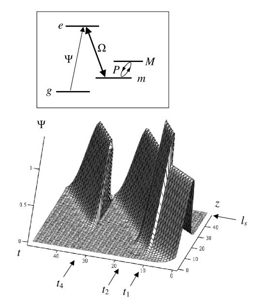
Figure 1: 3-d plot showing the spatial-temporal evolution of the signal field. Coordinates $z$, $t$ and amplitude $\Psi$ of the signal field are in arbitrary units. The instances of the control, $t_{1}$, $t_{2}$, and $t_{4}$, are indicated by arrows, as well as the end of the sample $z=l_{s}$. The excitation scheme of the four-level atom is shown in the inset (see the text for details).

References

- (1) M. Fleischhauer and M. D. Lukin, Phys. Rev. Lett. 84, 5094 (2000); Phys. Rev. A 65, 022314 (2002).
- (2) C. Liu, Z. Dutton, C. H. Behroozi, and L. V. Hau, Nature (London) 409, 490 (2001).
- (3) D. F. Phillips, A. Fleischhauer, A. Mair, R. L. Walsworth, and M. D. Lukin, Phys. Rev. Lett. 86, 783 (2001).
- (4) A. V. Turukhin, V. S. Sudarshanam, M. S. Shahriar, J. A. Musser, B. S. Ham, and P. R. Hemmer, Phys. Rev. Lett. 88, 023602 (2002).
- (5) T. Chaneliére, D. N. Matsukevich, S. D. Jenkins, S.-Y. Lan, T. A. B. Kennedy, and A. Kuzmich, Nature (London) 438, 833 (2005).
- (6) A. B. Matsko, Y. V. Rostovtsev, O. Kocharovskaya, A. S. Zibrov, and M. O. Scully, Phys. Rev. A 64, 043809 (2001).
- (7) R. N. Shakhmuratov and J. Odeurs, Phys. Rev. A 74, 043807 (2006).
- (8) R. Grobe, F. T. Hioe, and J. H. Eberly, Phys. Rev. Lett. 73, 3183 (1994).
- (9) R. N. Shakhmuratov and J. Odeurs, Phys. Rev. A 71, 013819 (2005).
- (10) E. Arimondo, Prog. Opt. 35, 257 (1996); S. E. Harris, Phys. Today 50 (7), 36 (1997).
- (11) L. Allen and J. H. Eberly, Optical Resonance and Two-Level Atoms (Wiley, New York, 1975).
- (12) J. Brendel, N. Gisin, W. Tittel, and H. Zbinden, Phys. Rev. Lett. 82, 2594 (1999).