Effects of imperfect noise correlations on decoherence-free subsystems: SU(2) diffusion model

Abstract

We present a model of an $N$-qubit channel where consecutive qubits experience correlated random rotations. Our model is an extension to the standard decoherence-free subsystems approach (DFS) which assumes that all the qubits experience the same disturbance. The variation of rotations acting on consecutive qubits is modeled as diffusion on the $\text{SU}(2)$ group. The model may be applied to spins traveling in a varying magnetic field, or to photons passing through a fiber whose birefringence fluctuates over the time separation between photons. We derive an explicit formula describing the action of the channel on an arbitrary $N$-qubit state. For $N=3$ we investigate the effects of diffusion on both classical and quantum capacity of the channel. We observe that nonorthogonal states are necessary to achieve the optimal classical capacity. Furthermore we find the threshold for the diffusion parameter above which coherent information of the channel vanishes.

I Introduction

A fruitful approach to protect quantum systems from decoherence introduced by uncontrolled interactions with the environment is to use symmetries exhibited by those interactions. When elementary quantum systems in an ensemble are coupled to the environment in an identical way, it is possible to identify certain collective degrees of freedom that turn out to be completely decoupled from the interaction, thus preserving quantum coherence. This approach is the basic idea behind decoherence-free subspaces and subsystems (DFSs) Palma et al. (1996); Bartlett et al. (2006) (for a review see Lidar and Whaley (2003)), which can be implemented in a number of physical scenarios including quantum dots Zanardi and Rossi (1998), atoms in a cavity Beige et al. (2000), ion traps Feng and Wang (2002) or photons transmitted through a birefringent fiber Bartlett et al. (2003). The existence of DFSs allows one to encode or communicate reliably both classical and quantum information, which has been demonstrated in first proof-of-principle experiments Kwiat et al. (2000).

The purpose of this paper is to go beyond the standard theory of DFSs and to analyze a scenario when the interactions of elementary systems with the environment are not necessarily identical. Specifically, we will consider a sequence of qubits affected by random unitary transformations. In the standard DFSs model all unitaries are the same, enabling one to apply the standard decomposition into multiplicity subspaces based on angular-momentum algebra. In this paper, we will assume that correlations between unitaries affecting consecutive qubits are characterized by a probability distribution describing isotropic diffusion on the SU(2) group. Such a distribution has a number of invariant properties that result in the existence of a single real parameter which defines the strength of correlations. This will enable us to investigate the continuous transition between the extreme regimes of perfect correlations and independent transformations of consecutive qubits.

The model introduced in this paper is a certain channel acting on a sequence of $N$ qubits. We derive its detailed description using angular momentum algebra, and analyze quantitatively the case of $N=3$ qubits. In particular we present numerical results concerning the classical capacity and present the optimal ensemble of states attaining it. Surprisingly, for imperfect correlations the optimal ensemble contains nonorthogonal states. The fact that the use of nonorthogonal states may be necessary for the optimal classical communication has been known Fuchs (1997), yet it is rather surprising that this effect appears in a channel constructed in such a natural way. We compare the optimal capacity with the one that can be achieved when one is restricted to the use of orthogonal states and indicate orthogonal states which perform almost optimal. We calculate and analyze the optimal coherent information, which provides certain information about the quantum capacity of the channel.

Results presented in this paper can be applied to different physical systems used for quantum communication, e.g. spins traveling in fluctuating external magnetic field, and photons traveling in a fiber with randomly varying birefringence. The model generalizes the standard DFS theory whenever the time separation between qubits sent through the channel is not negligible in comparison with the characteristic time of environment fluctuations. One can easily imagine such a situation in the case of spins traveling relatively slowly in randomly varying magnetic field. When it comes to photons, however, in most of present experiments the standard DFS approach seems satisfactory. The time separation of photons is typically several orders of magnitude smaller than the fluctuation time of birefringence, whose variations are caused by mechanical and thermal factors and hence by their nature are relatively slow. Nevertheless, our model might be relevant also in this setting, when large temporal separations between photons need to be introduced, or sequences of photons are long enough to reach the time scale of birefringence fluctuations.

The paper is organized as follows. We describe the model of imperfect correlations in Sec. II. In Sec. III investigate the structure of output states and give an explicit and efficient formula for calculating the action of the channel on an arbitrary $N$ qubit state. In Sec. IV we consider the example of three qubit communication, which is the smallest number of qubits allowing quantum information to be transmitted. Finally, Sec. V concludes the paper.

II Imperfect correlations

The standard model for collective depolarization of $N$ qubits described by a joint density matrix $\rho$ is given by the following map:

$$\mathcal{T}(\rho)=\int\textrm{d}U\ U^{\otimes N}\rho U^{\dagger\otimes N},$$ (1)

where $U$ is an $SU(2)$ matrix describing the rotation of a Bloch vector of a single qubit state and $\textrm{d}U$ is the Haar measure on the $SU(2)$ group. This operation inflicts a rotation which is completely random and identical for all qubits. In other words we may say that noise experienced by a given qubit is perfectly correlated with the noise experienced by all other qubits. We will refer to this map as the twirling map.

Let us now extend the above model in order to describe the situation where correlation of noise acting on different qubits is not perfect. We will assume that the density matrix $\rho$ of the qubits undergoes a unitary transformation given by a tensor product $U_{1}\otimes U_{2}\otimes\dots\otimes U_{N}$ averaged with a certain probability distribution $p(U_{1},U_{2},\ldots,U_{N})$. We will treat the sequence of $U_{i}$ as a discrete-time stochastic process with the Markov property, i.e. as a Markov chain Kampen (1992). Consequently the probability distribution for $U_{i}$ will only depend on $U_{i-1}$. Additionally, we will impose the stationarity condition on our process which means that the conditional probability distribution is described by the same function irrespectively of the index $i$. Thus the joint probability distribution is given by a product

$$p(U_{1},U_{2},\ldots,U_{N})=p(U_{N}|U_{N-1})\cdots p(U_{3}|U_{2})p(U_{2}|U_{1}).$$ (2)

We will consider an isotropic process, i.e. one that does not distinguish any element of the $SU(2)$ group, which is equivalent to the physical assumption that the fluctuations do not favor any particular form of depolarization. The isotropy condition requires that the conditional probability distribution $p(U_{i}|U_{i-1})=p(VU_{i}|VU_{i-1})=p(U_{i}V|U_{i-1}V)$, for every $V\in\text{SU}(2)$. This implies that

$$p(U_{i}|U_{i-1})=p(U_{i}U_{i-1}^{\dagger})=p(U_{i-1}^{\dagger}U_{i}),$$ (3)

where $p(U)$ is a certain probability distribution defined on the group SU(2), which fully characterizes our decoherence model.

As the explicit model for the distribution $p(U)$ we will take the solution to the diffusion equation on the group SU(2). This solution can be conveniently parameterized with a non-negative dimensionless time $t$ characterizing the diffusion strength. The explicit expression for the distribution $p_{t}(U)$ on the $\text{SU}(2)$ group at time $t$ reads Hogan and Chalker (2004):

$$p_{t}(U)=\sum_{j=0}^{\infty}(2j+1)\exp\left(-\frac{1}{2}j(j+1)t\right)\sum_{m=-j}^{j}\mathfrak{D}^{j}(U)_{m}^{m},$$ (4)

where $\mathfrak{D}^{j}(U)_{m}^{m^{\prime}}$ are rotation matrices of the $SU(2)$ group Devanthan (2002); Tung (2003); D.M.Brink (1968). The function $p_{t}(U)$ is invariant with respect to unitary transformations of its argument, i.e. $p_{t}(VUV^{\dagger})=p_{t}(U)$ for any $U,V\in\text{SU}(2)$. It depends only on the eigenvalues of $U$ which can be parameterized with a single angle $\xi$ as $e^{i\xi/2}$ and $e^{-i\xi/2}$. Then the sum over $m$ in Eq. (4), equal to the character of the $j$th irreducible representation, can be calculated explicitly as:

$$\sum_{m=-j}^{j}\mathfrak{D}^{j}(U)_{m}^{m}=\frac{\sin[(j+1/2)\xi]}{\sin(\xi/2)}.$$ (5)

The family of distributions $p_{t}(U)$ has the following convolution property:

$$\int\textrm{d}U\,p_{t_{1}}(U^{\prime}U^{\dagger})p_{t_{2}}(U)=p_{t_{1}+t_{2}}(U^{\prime}).$$ (6)

For $t\rightarrow 0$ the function $p_{t}(U)$ tends to a delta-like distribution peaked at identity, while for $t\rightarrow\infty$ it becomes uniform on the group. Therefore the limit $t\rightarrow 0$ corresponds to perfectly correlated depolarization specified in Eq. (1), and the opposite case of independent depolarization affecting each one of qubits is recovered when $t\rightarrow\infty$. We will be interested in perturbations in DFSs resulting from imperfect correlations characterized by a finite value of $t$.

III Channel action

We now proceed to write explicitly the action of the channel on an arbitrary $N$ qubit state $\rho$. The reasoning below is valid for an arbitrary isotropic function $p(U)$, and the exact form of $p(U)$ specified in Eq. (4) is not used until Eq. (16). The output state of the channel reads:

$$\mathcal{E}(\rho)=\int\textrm{d}U_{1}\int\textrm{d}U_{2}\dots\int\textrm{d}U_{N}p(U_{1},U_{2},\dots,U_{N})U_{1}\otimes U_{2}\otimes\dots\otimes U_{N}\ \rho\ U_{1}^{\dagger}\otimes U_{2}^{\dagger}\otimes\dots\otimes U_{N}^{\dagger}=$$

$$=\int\textrm{d}U_{1}\int\textrm{d}U_{2}\dots\int\textrm{d}U_{N}p(U_{2}|U_{1})p(U_{3}|U_{2})\dots p(U_{N}|U_{N-1})U_{1}\otimes U_{2}\otimes\dots\otimes U_{N}\ \rho\ U_{1}^{\dagger}\otimes U_{2}^{\dagger}\otimes\dots\otimes U_{N}^{\dagger}.$$

Taking into account Eq. (3), and introducing new variables $U_{i}^{\prime}=U_{i}U^{\dagger}_{i-1}$ we arrive at:

$$\mathcal{E}(\rho)=\int\textrm{d}U_{1}\int\textrm{d}U^{\prime}_{2}\dots\int\textrm{d}U^{\prime}_{N}p(U_{2}^{\prime})p(U_{3}^{\prime})\dots p(U_{N}^{\prime})\times\\ U_{1}\otimes(U_{2}^{\prime}U_{1})\otimes\dots\otimes(U^{\prime}_{N}U^{\prime}_{N-1}\dots U_{1})\ \rho\ U_{1}^{\dagger}\otimes(U_{1}^{\dagger}U_{2}^{\prime\dagger})\otimes\dots\otimes(U_{1}^{\dagger}U_{2}^{\prime\dagger}\dots U_{N}^{\prime\dagger})=\\ =\int\textrm{d}U^{\prime}_{N}p(U_{N}^{\prime})(\openone\otimes\dots\otimes U_{N}^{\prime})\dots\left(\int\textrm{d}U_{1}(U_{1}\otimes\dots\otimes U_{1})\ \rho\ (U_{1}^{\dagger}\otimes\dots\otimes U_{1}^{\dagger})\right)\dots(\openone\otimes\dots\otimes U_{N}^{\prime\dagger}).$$ (7)

The action of the channel can thus be written in a compact form:

$$\mathcal{E}(\rho)=\mathcal{I}_{N-1}\left(\mathcal{I}_{N-2}\left(\dots\mathcal{I}_{1}(\mathcal{T}(\rho))\dots\right)\right),$$ (8)

where:

$$\mathcal{I}_{i}(\rho)=\int\textrm{d}Up(U)\\ \times\underbrace{\openone\otimes\openone}_{i}\otimes\underbrace{U\otimes\dots\otimes U}_{N-i}\ \rho\ \underbrace{\openone\otimes\openone}_{i}\otimes\underbrace{U^{\dagger}\otimes\dots\otimes U^{\dagger}}_{N-i}.$$ (9)

It can be easily proven that thanks to the isotropy of the function $p(U)$ specified in Eq. (3), operations $\mathcal{I}_{i}$ commute with each other, i.e. $\mathcal{I}_{i}(\mathcal{I}_{k}(\rho))=\mathcal{I}_{k}(\mathcal{I}_{i}(\rho))$, and furthermore they commute with $\mathcal{T}$. This implies that $\mathcal{T}(\mathcal{E}(\rho))=\mathcal{E}(\mathcal{T}(\rho))$, which together with the fact that $\mathcal{T}(\mathcal{T}(\rho))=\mathcal{T}(\rho)$ leads us to the conclusion that $\mathcal{T}(\mathcal{E}(\rho))=\mathcal{E}(\rho)$. This means that the output state is invariant under the twirling map. We will say that it has a twirled structure.

The action of the twirling map in Eq. (8) allows us to restrict our considerations to input states having a twirled structure. Let us now describe the states $\rho_{\textrm{twirled}}=\mathcal{T}(\rho)$. For this purpose we use the following standard decomposition of the space of $N$ qubits:

$$\mathcal{H}^{\otimes N}=\bigoplus_{j=(N\bmod 2)/2}^{N/2}\underbrace{\mathcal{H}_{j}\oplus\ldots\oplus\mathcal{H}_{j}}_{d_{j}\textrm{ times}}=\bigoplus_{j=(N\bmod 2)/2}^{N/2}\mathcal{H}_{j}\otimes\mathbb{C}_{d_{j}},$$ (10)

where $\mathcal{H}_{j}$ is a representation subspace in which the $(2j+1)$-dimensional irreducible representation of $\text{SU}(2)$ acts, and $\mathbb{C}_{d_{j}}$ is the multiplicity subspace which is not affected by the action of $U^{\otimes N}$. The above decomposition allows us to use a basis $|j,m,\alpha\rangle$, where $j$ is the total angular momentum, $m$ is projection of angular momentum on the $z$ axis, and $\alpha$ labels representation subspaces that are equivalent, i.e. have identical $j$.

There are different ways of obtaining a given angular momentum by adding elementary $1/2$-spins of single qubits. If a given angular momentum is obtained by always adding the $i$-th spin-$1/2$ to the previously obtained total angular momentum of $i-1$ spins, these different ways correspond to different paths in the van Vleck diagram Karwowski and Shavitt (2003), shown in Fig. 1. Therefore $\alpha$ can be regarded as an index labelling different paths leading to equivalent representation subspaces. There are, however, alternative ways of specifying $\alpha$ which depend on the order of adding elementary $1/2$ spins. In the following calculations, it will be helpful to use different conventions for labelling equivalent representations, distinguished with a subscript $\{k\}$. In explicit terms, $\alpha_{\{k\}}$ will label equivalent representation subspaces which are obtained by first adding successively the first $k$ spins $1/2$, from number $1$ to $k$, then adding the last $N-k$ spins in the reverse order, from number $N$ to $k+1$, and finally combining these two groups together. The value of $\alpha_{\{k\}}$ is thus fully specified by a sequence $\{j_{1},j_{12},\dots,j_{1\dots k}\}\{j_{k+1\dots N},j_{k+2\dots N},\dots,j_{N}\}$, where $j_{i\dots k}$ is the total angular momentum after adding together spins from the number $i$ to $k$. Of course, a single particle spin is equal to $j_{i}=1/2$ for any $i$. Naturally, all the conventions for numbering equivalent subspaces, corresponding to a different choice of the $k$, are legitimate, yet the ability to switch between alternative conventions will make it possible to derive a compact formula for the action of the channel.

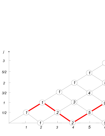
Figure 1: Van Vleck’s branching diagram describing addition of $N$ spins $1/2$. The $X$ and $Y$ axis corresponds to number of spins $N$ and the total spin $j$ respectively. The numbers in circles represent the multiplicity of given total angular momentum subspace (number of paths leading to it). An exemplary path $\{\frac{1}{2},1,\frac{1}{2},0,\frac{1}{2},1\}$ is marked with bold (red) line.

Using the decomposition given in Eq. (10) we can write any twirled state $\rho_{\textrm{twirled}}$ in the following way:

$$\rho_{\textrm{twirled}}=\mathcal{T}(\rho)=\bigoplus_{j=(N\bmod 2)/2}^{N/2}\frac{p_{j}}{2j+1}\openone_{\mathcal{H}_{j}}\otimes\rho_{j},$$ (11)

Denoting by $P_{j}$ a projection onto $\mathcal{H}_{j}\otimes\mathbb{C}_{d_{j}}$ we find the relations

$$p_{j} = \textrm{Tr}(P_{j}\rho),$$ (12)

$$\rho_{j} = \frac{1}{p_{j}}\textrm{Tr}_{\mathcal{H}_{j}}(P_{j}\rho P_{j}).$$ (13)

Because the action of $\mathcal{I}_{i}$ preserves the twirled structure, we may write the output state of the channel in an analogous form:

$$\mathcal{E}(\rho)=\mathcal{E}(\rho_{\textrm{twirled}})=\bigoplus_{j=(N\bmod 2)/2}^{N/2}\frac{p^{\textrm{out}}_{j}}{2j+1}\openone_{\mathcal{H}_{j}}\otimes\rho^{\textrm{out}}_{j}.$$ (14)

Therefore, the full description of the action of the channel amounts to writing $p_{j}^{\textrm{out}},\rho_{j}^{\textrm{out}}$ as a function of $p_{j},\rho_{j}$. Equivalently we may characterize the channel by its action on operators:

$$\begin{split}P_{J}^{\alpha,\alpha^{\prime}}&=\frac{1}{2J+1}\sum_{M=-J}^{J}|J,M,\alpha\rangle\langle J,M,\alpha^{\prime}|=\\ &=\frac{1}{2J+1}\openone_{\mathcal{H}_{J}}\otimes|\alpha\rangle\langle\alpha^{\prime}|\end{split}$$ (15)

since any twirled state can be written as their linear combination. As discussed before, we have freedom in choosing the convention for labels $\alpha$. The simplest expression is obtained if we specify how the channel acts on $P_{J}^{\alpha_{\{1\}},\alpha^{\prime}_{\{1\}}}$, and express the output in terms of the operators $P_{J}^{\alpha_{\{N-1\}},\alpha^{\prime}_{\{N-1\}}}$. The detailed derivation is presented in Appendix A, with the final formula in the form:

$$\begin{split}\mathcal{E}(P_{J}^{\alpha_{\{1\}},\alpha_{\{1\}}^{\prime}})&=\sum_{\begin{subarray}{c}j_{12}^{\prime}\\ j_{12}\end{subarray}}\ \dots\ \sum_{\begin{subarray}{c}j_{1\dots N-1}^{\prime}\\ j_{1\dots N-1}\end{subarray}}\sum_{J_{1}=|j_{1}-j_{2\dots N}|}^{j_{1}+j_{2\dots N}}\ \sum_{J_{2}=|j_{12}-j_{3\dots N}|}^{j_{12}+j_{3\dots N}}\ \dots\ \sum_{J_{N-1}=|j_{1\dots N-1}-j_{N}|}^{j_{1\dots N-1}+j_{N}}\ P_{J_{N-1}}^{\alpha_{\{N-1\}},\alpha_{\{N-1\}}^{\prime}}\times\\ &U(J_{1},2)^{j_{12}}_{j_{2\dots N}}U(J_{1},2)^{j^{\prime}_{12}}_{j^{\prime}_{2\dots N}}\ \dots\ U(J_{N-2},N-1)^{j_{1\dots N-1}}_{j_{N-1,N}}U(J_{N-2},N-1)^{j^{\prime}_{1\dots N-1}}_{j^{\prime}_{N-1,N}}\times\\ &R(t)^{J_{1},j_{1}^{\prime},j_{2\dots N}^{\prime}}_{J,j_{1},j_{2\dots N}}R(t)^{J_{2},j_{12}^{\prime},j_{3\dots N}^{\prime}}_{J_{1},j_{12},j_{3\dots N}}\ \dots\ R(t)^{J_{N-1},j_{1\dots N-1}^{\prime},j_{N}^{\prime}}_{J_{N-2},j_{1\dots N-1},j_{N}}\end{split}$$ (16)

where according to our convention $\alpha_{\{k\}}$, and $\alpha_{\{k\}}^{\prime}$ read:

$$\begin{split}\alpha_{\{k\}}&=\{j_{1},j_{12},\dots,j_{1\dots k}\}\{j_{k+1,\dots,N},j_{k+2,\dots,N},\dots,j_{N}\}\\ \alpha_{\{k\}}^{\prime}&=\{j_{1}^{\prime},j_{12}^{\prime},\dots,j_{1\dots k}^{\prime}\}\{j_{k+1,\dots,N}^{\prime},j_{k+2,\dots,N}^{\prime},\dots,j_{N}^{\prime}\},\end{split}$$ (17)

the functions $R(t)^{J_{k},j_{1}^{\prime},j_{2}^{\prime}}_{J,j_{1},j_{2}}$ are given in terms of Wigner $6j$ coefficients Devanthan (2002) as:

$$\begin{split}R(t)^{J_{k},j_{1}^{\prime},j_{2}^{\prime}}_{J,j_{1},j_{2}}=\sum_{j=|j_{2}-j_{2}^{\prime}|}^{j_{2}+j_{2}^{\prime}}(-1)^{J_{k}-J}(2j+1)(2J_{k}+1)\times\\ \exp\left(-\frac{1}{2}j(j+1)t\right)\left\{\begin{array}[]{ccc}j_{1}&J&j_{2}\\ j_{2}^{\prime}&j&j_{1}^{\prime}\end{array}\right\}\left\{\begin{array}[]{ccc}j_{1}&j_{1}^{\prime}&j\\ j_{2}^{\prime}&j_{2}&J_{k}\end{array}\right\},\end{split}$$ (18)

and $U(J,k)^{j_{1\dots k}}_{j_{k\dots N}}$ is a shorthand notation for specific coefficients $U(j_{1},j_{2},J,j_{3};j_{12},j_{23})$ used in adding three angular momenta Devanthan (2002), discussed in Appendix A):

$$U(J,k)^{j_{1\dots k}}_{j_{k\dots N}}=U(j_{1\dots k-1},1/2,J,j_{k+1\dots N};j_{1\dots k},j_{k\dots N}).$$ (19)

Recall also that all single particle spins $j_{i}=1/2$, which we kept implicit in Eq. (16) only to ease the understanding of the formula structure.

The formula (16), despite its lengthy appearance, enables an efficient calculation of the channel action even for a large number of qubits, which would be infeasible by inserting directly the formula for $p_{t}(U)$ into Eq. (7) and performing the integration.

IV Three qubits

The case $N=1$ of one qubit is trivial. The channel acts as completely depolarizing channel, hence its capacity both classical and quantum is zero. The case $N=2$ of two qubits was solved in Ref. Ball et al. (2004), where the optimal classical capacity was derived together with the optimal ensemble of states. The twirling operation in this case produces Werner states $\rho=(1+c)\openone/4-c|\psi^{-}\rangle\langle\psi^{-}|$. Imperfect correlations were introduced in that paper through a phenomenological shrinking factor $\eta$ multiplying the parameter $c$. Our general model predicts the same behavior, with the shrinking factor given explicitly by $\eta=e^{-t}$. Notice also that quantum capacity of this channel is zero since all multiplicity subspaces are one dimensional.

We will now investigate the action of the channel for three qubits, which is the lowest number with non-trivial equivalent representation subspaces. Adding three spins $1/2$ gives one subspace with $j=3/2$, which is the fully symmetric subspace, and two subspaces with $j=1/2$. The two-fold multiplicity of subspaces corresponding to $j=1/2$ enables one to preserve quantum superpositions. In the case of perfect correlations $t=0$ the channel acts as the identity in the multiplicity subspace Bartlett et al. (2006), which therefore forms a decoherence-free subsystem, making it possible to encode one qubit with the fidelity equal to one. The classical capacity of such a channel is equal to $\log_{2}3$, since we have three completely distinguishable output states: two orthogonal states of a qubit from the multiplicity subspace and one state from the fully symmetric subspace. When correlations between operations acting on consecutive qubits are not perfect the fidelity of the transmission as well as classical and quantum capacity will decrease. In this section we will derive analytical formulas for the fidelity of transmission through the channel as well as numerical and approximate analytical results for quantum and classical capacities of the channel.

For three qubits a general twirled state has the form:

$$\rho=\frac{p}{2}(\openone_{\mathcal{H}_{1/2}}\otimes\rho_{1/2})\oplus\frac{1-p}{4}\openone_{{\mathcal{H}}_{3/2}},$$ (20)

where $\rho_{1/2}$ is an arbitrary $2\times 2$ density matrix, and $0\leq p\leq 1$. Let us now specify a particular basis in the $j=1/2$ multiplicity subspace in which the operation ${\mathcal{E}}$ will have the simplest form. Let the state $|0\rangle$ correspond to the equivalent subspace labeled $\{j=1/2,\alpha=0\}$, obtained by combining the first two spins $1/2$ together to get the angular momentum $0$ and then adding the third spin with the total angular momentum $1/2$, while $|1\rangle$ corresponds to the equivalent subspace labeled $\{j=1/2,\alpha=1\}$, obtained by combining the first two spins to get the angular momentum $1$, and then adding the third spin to produce the total angular momentum $1/2$. For simplicity in what follows we will omit the identity operators acting in the representation subspaces. Instead of $\openone_{\mathcal{H}_{1/2}}\otimes\rho_{1/2}$ we will simply write a single qubit state $\rho_{1/2}$, and instead of $\openone_{\mathcal{H}_{3/2}}$ we will write $|2\rangle\langle 2|$. Our channel can be thus regarded as effectively a qutrit channel that preserves no coherence between subspaces $\{|0\rangle,|1\rangle\}$ and $\{|2\rangle\}$. The evolution of the state has the simplest form if we introduce the following basis in the qubit subspace:

$$|e_{1}\rangle=\frac{|0\rangle+\sqrt{3}|1\rangle}{2},\quad|e_{2}\rangle=\frac{\sqrt{3}|0\rangle-|1\rangle}{2}.$$ (21)

In order to describe the action of the channel it is sufficient to calculate its action on the extreme states whose convex combinations generate the entire set of twirled states. The extreme states are $|2\rangle\langle 2|$ and an arbitrary pure state $|\psi\rangle\langle\psi|$ in the qubit subspace, which we will parameterize as $|\psi\rangle=\cos(\theta/2)|e_{1}\rangle+\sin(\theta/2)e^{i\phi}|e_{2}\rangle$. Applying Eq. (16) to the three-qubit case yields:

$$\mathcal{E}(|2\rangle\langle 2|)=\left(\begin{array}[]{cc}\frac{1}{4}\left(1-e^{-2t}\right)&0\\ 0&\frac{1}{12}\left(3-4e^{-t}+e^{-2t}\right)\end{array}\right)\oplus\begin{array}[]{c}\frac{1}{6}\left(3+2e^{-t}+e^{-2t}\right)\end{array}$$ (22)

$$\begin{split}\mathcal{E}(|\psi\rangle\langle\psi|)=\left(\begin{array}[]{cc}\frac{1}{4}\left(1+e^{-2t}(1+2\cos\theta)\right)&\frac{1}{2}\sin\theta(e^{-t}\cos\phi-ie^{-2t}\sin\phi)\\ \frac{1}{2}\sin\theta(e^{-t}\cos\phi+ie^{-2t}\sin\phi)&\frac{1}{12}\left(3+8e^{-t}\sin^{2}(\theta/2)-e^{-2t}(1+2\cos\theta)\right)\end{array}\right)\oplus\\ \oplus\begin{array}[]{c}\frac{1}{6}\left(3-4e^{-t}\sin^{2}(\theta/2)-e^{-2t}(1+2\cos\theta)\right)\end{array},\end{split}$$ (23)

where the output matrix is written in the basis $|e_{1}\rangle$, $|e_{2}\rangle$, $|2\rangle$. This expression will be now used to calculate quantities characterizing the channel.

IV.1 Fidelity

Let us first calculate the transmission fidelity of a pure qubit state encoded in the multiplicity subspace. According to Eq. (23), with a probability $\frac{1}{6}[3-4e^{-t}\sin^{2}(\theta/2)-e^{-2t}(1+2\cos\theta)]$ the input qubit state is removed from the multiplicity subspace and transformed into the state $|2\rangle\langle 2|$. We can consider an effective one qubit channel $\mathcal{E}_{\textrm{eff}}$ by replacing the state $|2\rangle\langle 2|$ at the output with the maximally mixed state in the qubit space, given by $\openone/2$.

Since now we deal with an ordinary one qubit channel, i.e. a one qubit trace-preserving completely positive map, we may investigate its action in terms of an affine map on the Bloch vector. Written in the basis $|e_{1}\rangle,|e_{2}\rangle$, the output Bloch vector $\mathbf{r}_{\text{out}}$ can be expressed in terms of the input vector $\mathbf{r}_{\text{in}}$ as:

$$\mathbf{r}_{\text{out}}=\left(\begin{array}[]{lll}e^{-t}&0&0\\ 0&e^{-2t}&0\\ 0&0&\frac{2e^{-2t}+e^{-t}}{3}\end{array}\right)\mathbf{r}_{\text{in}}+\left(\begin{array}[]{l}0\\ 0\\ \frac{e^{-2t}-e^{-t}}{3}\end{array}\right).$$ (24)

The channel shrinks and translates the initial Bloch sphere. Notice that the shrinking is not isotropic and is weakest and strongest respectively in the $x$ and $y$ directions. The translation magnitude initially increases achieving the maximal value at $t=\ln(2)$ and then vanishes asymptotically.

The explicit expression for the fidelity of the output state is given by:

$$f(\theta,\phi,t)=\langle\psi|\ \mathcal{E}_{\textrm{eff}}(|\psi\rangle\langle\psi|)\ |\psi\rangle=\frac{1}{2}(1+\mathbf{r}_{\mathbf{\text{in}}}\cdot\mathbf{r}_{\text{out}})=\\ =\frac{1}{24}[12+5e^{-t}+7e^{-2t}+\\ +(e^{-2t}-e^{-t})(4\cos\theta-6\cos 2\phi\sin^{2}\theta+\cos 2\theta)].$$ (25)

and is depicted in Fig. 2. It is seen that the fidelity is optimized along meridians $\phi=0,\pi$, which is a consequence of the fact that shrinking is weakest in the $x$ direction. The highest transmission fidelity is achieved for states $\sqrt{5/8}|e_{1}\rangle\pm\sqrt{3/8}|e_{2}\rangle$, independently of the actual value of the diffusion time $t>0$.

We now compute the average fidelity of states lying on a great circle parameterized by the unit normal vector given in spherical coordinates $(\theta_{c},\phi_{c})$. This quantity is relevant when one needs to transmit a relative phase of an equally weighted superposition Huelga et al. (2002). The average great circle fidelity reads:

$$f_{c}(\theta_{c},\phi_{c})=\\ \frac{1}{24}\left[6\left(e^{-2t}+e^{-t}+2\right)+\left(e^{-2t}-e^{-t}\right)(1+3\cos 2\phi_{c})\sin^{2}\theta_{c}\right]$$ (26)

Thus it is a straightforward observation that the great circle parameterized by $(\theta_{c}=\pi/2,\phi_{c}=\pi/2)$ (the meridian in the $xz$ plane) is optimal and yields $f_{c}=(3+2e^{-t}+e^{-2t})/6$.

The average fidelity integrated over the entire Bloch sphere of input states with the uniform distribution is given by:

$$\langle f(t)\rangle=\frac{1}{18}\left(9+4e^{-t}+5e^{-2t}\right)$$ (27)

and it decreases monotonically with increasing diffusion strength. In the limit of strong diffusion $t\gg 1$ the the channel is completely depolarizing.

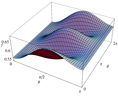
Figure 2: The fidelity $f(\theta,\phi,t=1)$ of states transmitted through an effective qubit channel $\mathcal{E}_{\textrm{eff}}$ as a function of the Bloch parameters $\theta$ and $\phi$ of the input state.

IV.2 Coherent information

We will now optimize the coherent information of the channel $\mathcal{E}$ in order to estimate its capacity for transmitting quantum information. Let us note that we now need to consider the full qutrit channel $\mathcal{E}$ acting according to Eqs. (22) and (23) rather than the effective one qubit channel $\mathcal{E}_{\textrm{eff}}$, as considering only the latter would lower the achievable quantum capacity.

Coherent information is defined as follows Nielsen and Chuang (2000):

$$I_{C}=\sup_{\rho}\left(S(\mathcal{E}(\rho))-S_{\textrm{env}}(\mathcal{E},\rho)\right),$$ (28)

where $S(\rho)=-\text{Tr}\left(\rho\log_{2}\rho\right)$ is the von Neumann entropy and $S_{\textrm{env}}$ is the entropy exchange Nielsen and Chuang (2000). The analytical optimization seems hard due to the complicated form of the Krauss operators Nielsen and Chuang (2000) our channel has. Nevertheless, one can easily notice that the optimal state $\rho$ in Eq. (28) will be supported on $\{|e_{1}\rangle,|e_{2}\rangle\}$ subspace, since the symmetric subspace $|2\rangle$ can be regarded as a purely classical degree of freedom and therefore cannot contribute to quantum capacity. Numerical optimization shows that the optimal state has the form:

$$\rho(\epsilon)=\epsilon|e_{1}\rangle\langle e_{1}|+(1-\epsilon)|e_{2}\rangle\langle e_{2}|.$$ (29)

We have optimized analytically the coherent information in the limit of weak diffusion (small $t$). In the case of no diffusion the state $\rho(\epsilon=1/2)$ maximizes the quantum capacity: $I_{C}=1$. We have expanded $I_{C}$ in a power series in $\epsilon$ around $\epsilon=1/2$ up to the second order and calculated the maximum. In the lowest order in $t$ (which includes also terms $t\log t$, reflecting the fact that the derivative of $I_{C}(t)$ diverges in $t=0$) the approximate input state parameter $\epsilon$ and the quantum capacity read:

$$I_{C} \approx 1-\frac{t}{3}\left(8-\log_{2}3+\frac{2}{\ln 2}-2\log_{2}t\right)$$ (30)

$$\epsilon \approx \frac{1}{2}+\frac{t}{6}\left(1-\frac{1}{\log_{2}3}\right)$$ (31)

Figure 3: Coherent information $I_{C}$ as a function of diffusion time $t$. The numerical solution is marked with the solid line, the analytical approximation given by Eq. (30) is marked with the dashed line.

Numerical results depicted in Fig. 3 indicate that coherent

information drops to strictly zero for diffusion time $t>0.275$, which strongly suggest that in this regime no quantum communication is possible. Since our channel is not degradable Devetak and Shor (2005) it could happen that the quantum capacity is not zero even though the coherent information vanishes, see e.g. Ref Barnum et al. (1998).

Figure 4: The parameter $\epsilon$ of the input state maximizing the coherent information $I_{C}$. The numerical solution is marked with the solid line, the analytical approximation given in Eq. (31) is marked with the dashed line.

IV.3 Classical capacity

The classical capacity of a quantum channel can be calculated using the Holevo-Schumacher-Westmoreland Schumacher and Westmoreland (1997); Nielsen and Chuang (2000) formula:

$$C=\sup_{\{p_{i},\rho_{i}\}}\left[S\left(\mathcal{E}\left(\sum_{i}p_{i}\rho_{i}\right)\right)-\sum_{i}p_{i}S(\mathcal{E}\left(\rho_{i})\right)\right],$$ (32)

where the supremum is taken over all ensembles $\{p_{i},\rho_{i}\}$. Let $\tilde{C}=S\left(\mathcal{E}\left(\sum_{i}p_{i}\rho_{i}\right)\right)-\sum_{i}p_{i}S(\mathcal{E}\left(\rho_{i})\right)$ denote the expression that is optimized in Eq. (32). In order to achieve the supremum it is enough to use $d^{2}$ pure states, where $d$ is the dimension of the input Hilbert space Verstraete (2002). In our case the maximum number of pure stares needed to achieve the supremum is five: four in the qubit subspace and additionally the symmetric state $|2\rangle$. We implemented numerical optimization of the classical capacity, which for all diffusion times $t$ yielded three-element optimal ensembles containing only two states from the qubit subspace. Furthermore, the sub-ensemble in the qubit subspace was composed of states given by:

$$\begin{split}|\psi_{1}\rangle&=\cos(\theta/2)|e_{1}\rangle+\sin(\theta/2)|e_{2}\rangle\\ |\psi_{2}\rangle&=\cos(\theta/2)|e_{1}\rangle-\sin(\theta/2)|e_{2}\rangle\end{split}$$ (33)

and equal weights, which we will denote by $q$. The parameters $q$ and $\theta$ are functions of $t$.

For $t>0$ the optimal states $|\psi_{1}\rangle$ and $|\psi_{2}\rangle$ turn out to be non-orthogonal. In order to judge how significant this nonorthogonality is for the channel transmission, let us compare the optimal capacity with the capacity attainable when composing the input ensemble from a pair of orthogonal states in the qubit subspace and the symmetric state $|2\rangle$. The optimal orthogonal states for transmission in the qubit subspace are $1/\sqrt{2}(|e_{1}\rangle\pm|e_{2}\rangle)$. As seen in Fig. 5, the capacity obtained using these states is very close to the absolute optimum. However, a different choice of orthogonal states can significantly deteriorate the capacity, with the worst case corresponding to the states $1/\sqrt{2}(|e_{1}\rangle\pm i|e_{2}\rangle)$. The best and the worst performance of these pairs can be explained intuitively by the anisotropy of the effective qubit channel ${\mathcal{E}}_{\textrm{eff}}$: the optimal orthogonal states lay on the $x$ axis characterized by the weakest shrinking, while the worst ones on the $y$ axis where the shrinking is strongest. This argument is of course not rigorous, as we are dealing here with the full qutrit channel rather than the effective one ${\mathcal{E}}_{\textrm{eff}}$ in the qubit subspace. While in the limit $t=0$ of no diffusion any pair of orthogonal states performs equally well, this invariance is broken for $t>0$ owing to the asymmetric character of the channel. However, the particular choice of the orthogonal states given by $1/\sqrt{2}(|e_{1}\rangle\pm|e_{2}\rangle)$ performs close to optimum for any diffusion strength.

In order to obtain an approximate analytical solution we expand $\tilde{C}=\tilde{C}(\theta,q,t)$ in a power series up to the second order in $(\theta,q)$ around $(\pi/2,1/3)$ and optimize analytically. This yields an approximate solution for a weak diffusion, given by:

$$q \approx \frac{1}{3}+\frac{t}{108}\left(5+\frac{7}{4\log_{2}3}+\ln t\right)$$ (34)

$$\theta \approx \frac{\pi}{2}-\frac{t}{12}\left(1-\log_{2}3+2\ln t\right)$$ (35)

Figure 5: The classical capacity of the quantum channel $C$ as a function of diffusion time $t$. The solid line depicts numerical results, the dashed line depicts the approximate analytical solution from Eq. (36), while dashed-dotted and dotted lines represent capacities obtained using respectively the best and the worst pairs of orthogonal states. Notice that using proper orthogonal states allows one almost to achieve the optimal capacity.

Figure 6: The optimal weight $q$ and the optimal Bloch parameter $\theta$, given in Eq. (33), of input states belonging to the $j=1/2$ multiplicity subspace maximizing classical information transmission. The solid lines depict numerical results, dashed lines represent approximate analytical solutions, given in Eqs. (34) and (35). Notice that for $t>0$ the states are nonorthogonal.

A comparison between numerical and approximate analytical solutions is shown in Fig. 6. The graphs show a good agreement of analytical solution with numerical results. Substituting Eqs. (34) and (35) into $\tilde{C}(\theta,q,t)$ and retaining leading terms yields an approximate formula for the capacity:

$$C\approx\log_{2}3+\frac{t}{9}\left(1-\frac{14+11\ln 3}{2\ln 2}+7\log_{2}t\right),$$ (36)

which is compared with numerical results in Fig. 5.

V Conclusions and discussion

In this paper we have introduced a model an $N$ qubit channel with imperfectly correlated noise, i.e. rotations inflicting consecutive qubits are subjected to the process of diffusion. We have given an explicit formula for the action of the channel on an arbitrary $N$ qubit state and for $N=3$ we calculated the optimal classical and quantum capacities and the states which are optimal for communication. Interestingly, we have observed that classical capacity is maximized when using nonorthogonal states. Additionally, we analyzed the robustness of different orthogonal states, which in the case of no diffusion (perfect noise correlation) are optimal for classical communication. We have indicated the most robust orthogonal states which perform almost optimal for all diffusion times. We have also found a threshold for the diffusion time above which the coherent information is zero and hence most probably no quantum information can be transmitted.

The model is a very natural extension of the standard DFS theory, and it can be applied to any physical situation when the action of the environment on the qubits can be described by a stationary Markov chain of $\text{SU}(2)$ matrices, and where the transition probability is described by an isotropic diffusion process on the $\text{SU}(2)$ group. This is equivalent to the assumption that consecutive matrices are the result of an isotropic random walk on the $\text{SU}(2)$ group (see Saloff-Coste (2001) for a review on random walks on groups). The assumption can be justified for systems we discussed in the introduction: spins traveling in the presence of randomly varying magnetic field and photons transmitted through a fiber with birefringence fluctuations. In both cases consecutive qubits (spins or photons) experience varying rotations in the channel, caused by fluctuations of the magnetic field or by birefringence. These multiple small random contributions lead to the random walk of the effective matrix describing the action of the channel on consecutive qubits. If these fluctuations are isotropic then obviously the random walk is isotropic and it leads to the model we have presented. Furthermore, even if fluctuations are anisotropic the effective random walk will be isotropic thanks to the assumption that the channel is long enough to completely depolarize every single qubit transmitted. This remark is relevant for fibers where the birefringence fluctuations are typically modeled as anisotropic Wai and Menyuk (1995), with the principal axis corresponding to a linear polarization. However, if such a fluctuation occurs at some intermediate point of a sufficiently long fiber, random polarization rotations introduced by the preceding and the following sections of the fiber should make such fluctuations isotropic.

Appendix A Derivation of the action of the channel $\mathcal{E}$ on operators $P_{J}^{\alpha,\alpha^{\prime}}$

According to Eq. (8) the action of the channel can be expressed as a composition of operations $\mathcal{I}_{i}$ defined in Eq. (9). Let us calculate the action of $\mathcal{I}_{i}$ on operators $P_{J}^{\alpha,\alpha^{\prime}}$ introduced in Eq. (15). Since $\mathcal{I}_{i}$ acts non trivially only on the last $N-i$ qubits it will be convenient to number equivalent representation subspaces using the convention described in Sec. III, and write explicitly $\alpha_{\{i\}}=\{j_{1},j_{12},\dots,j_{1\dots i}\}\{j_{i+1,\dots,N},j_{i+2,\dots,N},\dots,j_{N}\}$. The first step is to calculate the action of $\mathcal{I}_{i}$ on $P_{J}^{\alpha_{\{i\}},\alpha^{\prime}_{\{i\}}}$:

$$\mathcal{I}_{i}(P_{J}^{\alpha_{\{i\}},\alpha^{\prime}_{\{i\}}})=\int\textrm{d}Up_{t}(U)\times\\ \underbrace{\openone\otimes\openone}_{i}\otimes\underbrace{U\otimes\dots\otimes U}_{N-i}\ P_{J}^{\alpha_{\{i\}},\alpha^{\prime}_{\{i\}}}\ \underbrace{\openone\otimes\openone}_{i}\otimes\underbrace{U^{\dagger}\otimes\dots\otimes U^{\dagger}}_{N-i}.$$ (37)

Using $\alpha_{\{i\}}$ for labelling equivalent representations allows us to decompose the state $|J,M,\alpha_{\{i\}}\rangle$ using Clebsch-Gordan coefficients, denoted here with square brackets, according to:

$$\begin{split}|J,M,\alpha_{\{i\}}\rangle&=\sum_{m_{1\dots i}=-j_{1\dots i}}^{j_{i+1\dots N}}\left[\begin{array}[]{ccc}j_{1\dots i}&j_{i+1\dots N}&J\\ m_{1\dots i}&m_{i+1\dots N}&M\end{array}\right]\times\\ &\underbrace{|j_{1\dots i},m_{1\dots i},\alpha_{1}\rangle}_{i\textrm{ first qubits}}\otimes\underbrace{|j_{i+1\dots N},m_{i+1\dots N},\alpha_{2}\rangle}_{N-i\textrm{ last qubits}}.\end{split}$$ (38)

The total angular momenta of the first $i$ and the last $N-i$ qubits, given respectively by $j_{1\dots i}$ and $j_{i+1\dots N}$ are uniquely determined by $\alpha_{\{i\}}$. Similarly, the labelling of equivalent subspaces $\alpha_{1}$, $\alpha_{2}$ within each block of qubits is determined by $\alpha_{\{i\}}$ via the following relations: $\alpha_{1}=\{j_{1},j_{12},\dots,j_{1\dots i-1}\}\{j_{i}\}$, $\alpha_{2}=\{j_{i+1}\}\{j_{i+2\dots N},\dots,j_{N}\}$ (remember that $j_{i}=1/2$ for any $i$). An analogous decomposition can be applied to $|J,M,\alpha^{\prime}_{\{i\}}\rangle$.

The next step is to write the operator $P_{J}^{\alpha_{\{i\}},\alpha^{\prime}_{\{i\}}}$ using the decomposition given in Eq. (38). The operation $\mathcal{I}_{i}$ acts trivially on the first $i$ qubits, while the action of $U^{\otimes(N-i)}$ on the last $N-i$ qubits can be written with the help of Wigner rotation matrix $\mathfrak{D}^{j}(U)^{m^{\prime}}_{m}$. By substituting the explicit form of $p_{t}(U)$ given in Eq. (4) into Eq. (37) and using properties of Clebsch-Gordan coefficients, Wigner rotation matrices, and $6j$ Wigner symbols (see chapters 3,5,7 in Ref. Devanthan (2002)) we arrive after some lengthy calculations at a compact formula:

$$\mathcal{I}_{i}(P_{J}^{\alpha_{\{i\}},\alpha^{\prime}_{\{i\}}})=\sum_{J_{i}=|j_{1\dots i}-j_{i+1\dots N}|}^{j_{1\dots i}+j_{i+1\dots N}}R(t)^{J_{i},j_{1\dots i}^{\prime},j_{i+1\dots N}^{\prime}}_{J,j_{1\dots i},j_{i+1\dots N}}P_{J_{i}}^{\alpha_{\{i\}},\alpha^{\prime}_{\{i\}}},$$ (39)

where:

$$\begin{split}R(t)^{J_{i},j_{1}^{\prime},j_{2}^{\prime}}_{J,j_{1},j_{2}}=\sum_{j=|j_{2}-j_{2}^{\prime}|}^{j_{2}+j_{2}^{\prime}}(-1)^{J_{i}-J}(2j+1)(2J_{i}+1)\times\\ \exp\left(-\frac{1}{2}j(j+1)t\right)\left\{\begin{array}[]{ccc}j_{1}&J&j_{2}\\ j_{2}^{\prime}&j&j_{1}^{\prime}\end{array}\right\}\left\{\begin{array}[]{ccc}j_{1}&j_{1}^{\prime}&j\\ j_{2}^{\prime}&j_{2}&J_{i}\end{array}\right\}\end{split}$$ (40)

and the curly brackets denote Wigner $6j$ symbols. Notice that the expression derived in Eq. (39) can be used only if the index $i$ in the operation $\mathcal{I}_{i}$ is identical with the index $i$ specifying the convention for numbering equivalent subspaces $\alpha_{\{i\}}$. If we want to apply Eq. (39) to calculate the full action of the channel, given by

$$\mathcal{E}(P_{J}^{\alpha,\alpha^{\prime}})=\mathcal{I}_{N-1}(\dots\mathcal{I}_{2}(\mathcal{I}_{1}(P_{J}^{\alpha,\alpha^{\prime}}))\dots)$$ (41)

it is convenient to start from $P_{J}^{\alpha_{\{1\}},\alpha^{\prime}_{\{1\}}}$ for the representation of the input state, and then to adjust the convention after each step. To carry on this procedure we need to be able to express operators $P_{J}^{\alpha_{\{i-1\}},\alpha^{\prime}_{\{i-1\}}}$ in terms of $P_{J}^{\alpha_{\{i\}},\alpha^{\prime}_{\{i\}}}$.

The necessary expression can be derived using the standard formalism for adding three angular momenta. Consider three spins $j_{1}$, $j_{2}$, and $j_{3}$. One can write a basis using the total angular momentum of all spins in two different ways depending on the order in which spins were added together. A ket $|j_{1},(j_{2}j_{3})j_{23},J,M\rangle$ corresponds to a state with the total angular momentum $J$ and projection on the $z$ axis $M$, when spins $j_{2}$, $j_{3}$ were first coupled together yielding the angular momentum $j_{23}$ and finally the spin $j_{1}$ was added resulting in the total angular momentum $J$. Analogously $|(j_{1}j_{2})j_{12},j_{3},J,M\rangle$ corresponds to the situation when first spins $j_{1}$ and $j_{2}$ are added and subsequently the spin $j_{3}$ joins them. A unitary operation $U(j_{1},j_{2},J,j_{3};j_{12},j_{23})$ that transforms between these bases:

$$|j_{1},(j_{2}j_{3})j_{23},J,M\rangle=\sum_{j_{12}=|j_{1}-j_{2}|}^{j_{1}+j_{2}}U(j_{1},j_{2},J,j_{3};j_{12},j_{23})\\ \times|(j_{1}j_{2})j_{12},j_{3},J,M\rangle$$ (42)

can be expressed using $6j$ Wigner symbols as:

$$U(j_{1},j_{2},J,j_{3};j_{12},j_{23})=\sqrt{(2j_{12}+1)(2j_{23}+1)}\\ \times(-1)^{-(j_{1}+j_{2}+J+j_{3})}\left\{\begin{array}[]{ccc}j_{1}&j_{2}&j_{12}\\ j_{3}&J&j_{23}\end{array}\right\}$$ (43)

Specializing these general formulas to our calculation (i.e. replacing $j_{1}$ with $j_{1\dots i-1}$, $j_{2}$ with $1/2$ and $j_{3}$ with $j_{i+1,\dots N}$) we can write:

$$P_{J}^{\alpha_{\{i-1\}},\alpha_{\{i-1\}}^{\prime}}=\sum_{\begin{subarray}{c}j_{1\dots i}^{\prime}\\ j_{1\dots i}\end{subarray}}U(J,i)^{j_{1\dots i}}_{j_{i\dots N}}P_{J}^{\alpha_{\{i\}},\alpha_{\{i\}}^{\prime}}U(J,i)^{j^{\prime}_{1\dots i}}_{j^{\prime}_{i\dots N}}.$$ (44)

where the coefficients $U(J,k)^{j_{1\dots k}}_{j_{k\dots N}}$ are defined in Eq. (19). For completeness let us also write an inverse relation allowing for the lowering of the index $i$:

$$P_{J}^{\alpha_{\{i\}},\alpha_{\{i\}}^{\prime}}=\sum_{\begin{subarray}{c}j_{i\dots N}^{\prime}\\ j_{i\dots N}\end{subarray}}U(J,i)^{j_{1\dots i}}_{j_{i\dots N}}P_{J}^{\alpha_{\{i-1\}},\alpha_{\{i-1\}}^{\prime}}U(J,i)^{j^{\prime}_{1\dots i}}_{j^{\prime}_{i\dots N}}.$$ (45)

Equipped with the above formulas we can now calculate the action of the complete channel. For the input state expressed as a combination of operators $P_{J}^{\alpha_{\{1\}},\alpha_{\{1\}}^{\prime}}$, the action of the operation ${\mathcal{I}}_{1}$ is, according to Eq. (39) given by:

$$\mathcal{I}_{1}(P_{J}^{\alpha_{\{1\}},\alpha_{\{1\}}^{\prime}})=\sum_{J_{1}=|j_{1}-j_{2\dots N}|}^{j_{1}+j_{2\dots N}}R(t)^{J_{1},j^{\prime}_{1},j_{2\dots N}^{\prime}}_{J,j_{1},j_{2\dots N}}P_{J_{1}}^{\alpha_{\{1\}},\alpha_{\{1\}}^{\prime}}.$$ (46)

In order to calculate the action of $\mathcal{I}_{2}$ we need to represent $P_{J}^{\alpha_{\{1\}},\alpha_{\{1\}}^{\prime}}$ in terms of operators $P_{J}^{\alpha_{\{2\}},\alpha_{\{2\}}^{\prime}}$. Using Eq. (44) yields:

$$P_{J}^{\alpha_{\{1\}},\alpha_{\{1\}}^{\prime}}=\sum_{\begin{subarray}{c}j_{12}^{\prime}\\ j_{12}\end{subarray}}U(J,2)^{j_{12}}_{j_{2\dots N}}P_{J}^{\alpha_{\{2\}},\alpha_{\{2\}}^{\prime}}U(J,2)^{j^{\prime}_{12}}_{j^{\prime}_{2\dots N}}.$$ (47)

We may now apply the operation $\mathcal{I}_{2}$, whose action on the operators $P_{J}^{\alpha_{\{2\}},\alpha_{\{2\}}^{\prime}}$ is again given by Eq. (39). The combined action of $\mathcal{I}_{2}$ and $\mathcal{I}_{1}$ thus reads:

$$\begin{split}\mathcal{I}_{2}(\mathcal{I}_{1}(P_{J}^{\alpha_{\{1\}},\alpha_{\{1\}}^{\prime}}))&=\sum_{J_{1}=|j_{1}-j_{2\dots N}|}^{j_{1}+j_{2\dots N}}R(t)^{J_{1},j_{1}^{\prime},j_{2\dots N}^{\prime}}_{J,j_{1},j_{2\dots N}}\sum_{\begin{subarray}{c}j_{12}^{\prime}\\ j_{12}\end{subarray}}U(J_{1},2)^{j_{12}}_{j_{2\dots N}}U(J_{1},2)^{j^{\prime}_{12}}_{j^{\prime}_{2\dots N}}\sum_{J_{2}=|j_{12}-j_{3\dots N}|}^{j_{12}+j_{3\dots N}}R(t)^{J_{2},j_{12}^{\prime},j_{3\dots N}^{\prime}}_{J_{1},j_{12},j_{3\dots N}}\ P_{J_{2}}^{\alpha_{\{2\}},\alpha_{\{2\}}^{\prime}}\end{split}$$ (48)

Iterating this procedure yields the explicit formula for the action of the channel ${\mathcal{E}}$ given in Eq. (16). Notice in this formula the output state is expressed in terms of operators $P_{J}^{\alpha_{\{N-1\}},\alpha_{\{N-1\}}^{\prime}}$. If desired this expression can be converted back to the representation of operators $P_{J}^{\alpha_{\{1\}},\alpha_{\{1\}}^{\prime}}$ by applying repeatedly Eq. (45).

References

• Palma et al. (1996) G. M. Palma, K.-A. Suominen, and A. K. Ekert, Proc. Roy. Soc. London Ser. A 452, 567 (1996); P. Zanardi and M. Rasetti, Phys. Rev. Lett. 79, 3306 (1997); L.-M. Duan and G.-C. Guo, Phys. Rev. Lett. 79, 1953 (1997); D. A. Lidar, I. L. Chuang, and K. B. Whaley, Phys. Rev. Lett. 81, 2594 (1998); E. Knill, R. Laflamme, and L. Viola, Phys. Rev. Lett. 84, 2525 (2000a); E. Knill, R. Laflamme, and L. Viola, Phys. Rev. Lett. 84, 2525 (2000b).
• Bartlett et al. (2006) S. D. Bartlett, T. Rudolph, and R. W. Spekkens, Rev. Mod. Phys. 79, 555 (2006).
• Lidar and Whaley (2003) D. A. Lidar and K. B. Whaley, Decoherence-Free Subspaces and Subsystems in Irreversible Quantum Dynamics, vol. 622 of Springer Lecture Notes in Physics (2003).
• Zanardi and Rossi (1998) P. Zanardi and F. Rossi, Phys. Rev. Lett. 81, 4752 (1998).
• Beige et al. (2000) A. Beige, D. Braun, B. Tregenna, and P. L. Knight, Phys. Rev. Lett. 85, 1762 (2000).
• Feng and Wang (2002) M. Feng and X. Wang, Phys. Rev. A 65, 044304 (2002).
• Bartlett et al. (2003) S. D. Bartlett, T. Rudolph, and R. W. Spekkens, Phys. Rev. Lett. 91, 027901 (2003).
• Kwiat et al. (2000) P. G. Kwiat, A. J. Berglund, J. B. Altepeter, and A. G. White, Science 290, 498 (2000); D. Kielpinski, V. Meyer, M. A. Rowe, C. A. Sackett, W. M. Itano, C. Monroe, and D. J. Wineland, Science 291, 1013 (2001); L. Viola, E. M. Fortunato, M. A. Pravia, E. Knill, R. Laflamme, and D. G. Cory, Science 293 (2001); E. M. Fortunato, L. Viola, J. Hodges, G. Teklemariam, and D. G. Cory, New. J. Phys. 4, 5 (2002); K. Banaszek, A. Dragan, W. Wasilewski, and C. Radzewicz, Phys. Rev. Lett. 92, 257901 (2004); M. Bourennane, M. Eibl, S. Gaertner, C. Kurtsiefer, A. Cabello, and H. Weinfurter, Phys. Rev. Lett. 92, 107901 (2004); C. F. Roos, M. Chwalla, K. Kim, M. Riebe, and R. Blatt, Nature 443, 316 (2006).
• Fuchs (1997) C. A. Fuchs, Phys. Rev. Lett. 79, 1162 (1997).
• Kampen (1992) N. G. V. Kampen, Stochastic processes in physics and chemistry (Elsevier B.V., 1992).
• Hogan and Chalker (2004) P. M. Hogan and J. T. Chalker, J. Phys A: Math. Gen. 37, 11751 (2004).
• Devanthan (2002) V. Devanthan, Angular Momentum Techniques in Quantum Mechanics (Kluwer Academic Press, 2002).
• Tung (2003) W.-K. Tung, Group Theory in Physics (World Scientific, 2003).
• D.M.Brink (1968) G. S. D.M.Brink, Angular Momentum (Clarendon Press, Oxford, 1968).
• Karwowski and Shavitt (2003) J. A. Karwowski and I. Shavitt, Handbook of Molecular Physics and Quantum Chemistry, vol. 2 (John Wiley & Sons, 2003).
• Ball et al. (2004) J. Ball, A. Dragan, and K. Banaszek, Phys. Rev. A 69, 042324 (2004).
• Huelga et al. (2002) S. F. Huelga, M. B. Plenio, and J. A. Vaccaro, Phys. Rev. A 65, 042316 (2002).
• Nielsen and Chuang (2000) M. A. Nielsen and I. L. Chuang, Quantum Computation and Quantum Information (Cambridge University Press, 2000).
• Devetak and Shor (2005) I. Devetak and P. Shor, Commun. Math. Phys. 256, 287 (2005).
• Barnum et al. (1998) H. Barnum, M. A. Nielsen, and B. Schumacher, Phys. Rev. A 57, 4153 (1998).
• Schumacher and Westmoreland (1997) B. Schumacher and M. D. Westmoreland, Phys. Rev. A 56, 131 (1997).
• Verstraete (2002) F. Verstraete, Ph.D. thesis, Katholike Universiteit Leuven (2002).
• Saloff-Coste (2001) L. Saloff-Coste, Notices of the AMS 48, 968 (2001).
• Wai and Menyuk (1995) P. K. A. Wai and C. R. Menyuk, Optics Letters 20, 2493 (1995).