On EPR paradox, Bell’s inequalities, and experiments that prove nothing
Abstract
This article shows that the there is no paradox. Violation of Bell’s inequalities should not be identified with a proof of non locality in quantum mechanics. A number of past experiments is reviewed, and it is concluded that the experimental results should be re-evaluated. The results of the experiments with atomic cascade are shown not to contradict the local realism. The article points out flaws in the experiments with down-converted photons. The experiments with neutron interferometer on measuring the “contextuality” and Bell-like inequalities are analyzed, and it is shown that the experimental results can be explained without such notions. Alternative experiment is proposed to prove the validity of local realism.
1 Introduction
The EPR paradox [1] was formulated in the following way: with the common sense logic we can predict that a particle can have precisely defined position and momentum simultaneously, however quantum mechanics (QM) forbids it because operators and corresponding to position and momentum are not commuting, . Therefore QM is not complete.
The common sense logic was applied to the quantum mechanical state of two particles, which interacted at some moment in the past and then flew far apart. The distance becomes so large after the separation, that there are no more interaction between the particles.
The state of the two particles is described by a wave function , where are coordinates of the particles. This wave function can be expanded over the eigen functions of the momentum operator of the first particle
| (1) |
where are the expansion coefficients. Although particles flew far apart, their wave function, according to QM, is not a product of two independent functions. It is a superposition of such products. This superposition is used to be called “entangled” state. EPR devised a model where coefficients are also the eigen functions of the momentum operator . Therefore, if measurement with the first particle reveals it in the state with a fixed momentum , then the second particle is also in the state with the fixed momentum . According to EPR logic, the second particle does not interact with the first one, therefore it has momentum independently of the measurements on the first particle.
Similar consideration with the expansion over the eigen functions of the position operator shows that the measurement of the position of the first particle immediately predicts the position of the second one. Since the second particle does not interact with the first one, position and momentum of the second particle exist independently of the measurements on the first one. However, this case is impossible because of the noncommutativity of position and momentum operators. Therefore, we must admit that either QM is incomplete and should be improved by introducing some not yet known (hidden) parameters, or that QM is complete but there is some kind of instant action at a distance that puts the second particle into the state consistent with the apparatus measuring the first particle.
Such action at a distance must exist only if one accepts Copenhagen interpretation of QM. According to this interpretation, performing a measurement in one part of space immediately leads to a reduction of the entangled state to a single term everywhere in space. We can avoid such drastic instantaneous reduction, if we further follow the EPR logic. According to this logic, if the measurement on the first particle reveals it in the state , then the second particle is in the state . This wave function belongs to the second particle independently of the measurements performed on the first one. But, if the second particle is described by , the first particle can only be in the state . Therefore the state of the two particles before any measurements is described by the single product term of the sum (1). The measurement on the first particle reveals only which term is present in the given event.
Bohm-Aharonov [2] reformulated the EPR paradox in terms of the spin components of two particles. They considered a molecule with zero angular momentum and its decay into two spin 1/2 atoms A and B, that fly far apart in opposite directions. According to [2], if the atom A is transmitted through an analyzer oriented along a vector , then the spin of the atom B is directed with certainty along the vector . This result looks very natural from QM point of view, because we always can choose direction as a quantization axis. The spin of the particle A is directed along or opposite , i.e. its projection on is . Therefore, the projection of the spin of the particle B is . In the following we can imagine that the projection has plus sign when the particle is counted by the detector after the analyzer, and minus sign when it is not (it can then be counted by a different nearby detector, which detects particles reflected by the analyzer).
J.S. Bell [3] considered this situation as a predetermined one. He decided to check whether it is really possible to introduce such a hidden parameter , with which we can exactly predict whether particle A will have projection +1/2 or -1/2 on the direction , and therefore particle B will have projections on the same direction. Situation becomes more difficult when the analyzer for the particle B is aligned along a vector noncollinear to . Then the quantization axis for the particle B is along , projections of the spin on this axis are the same as on the axis , but now the signs of the projections are not necessarily opposite to the signs of the projections of the spin of the particle A on the axis . Bell suggested that the hidden parameter predetermined the sign of the projections of the two particles on vectors and . He introduced well defined functions and such that for every fixed the result of measurement of two spin components can be described by a predetermined product . If a distribution of is described by a classical probability density , then the result of the measurement of projections of two spins on axes and is given by the average
The question is: is it possible to find such classical distribution that the classical average ([3]2) is equal to the quantum mechanical expectation value for a singlet, i.e. entangled, state of two particles:
where are the spin operators (the Pauli matrices) for particles A and B. In the attempt to answer this question, Bell formulated his famous inequality and found that the inequality must be violated because (see [3], p.19)
“the quantum mechanical expectation value cannot be represented, either accurately or arbitrary closely, in the form ([3]2).”
Therefore
“there must be a mechanism whereby the setting of one measuring device can influence the reading of another measurement, however remote. More over, he signal involved must propagate instantaneously, so that such a theory could not be Lorentz invariant.”
Notwithstanding how strange this statement looks to a physicist, it was so attractive that it gave birth to a flood of experimental work devoted to demonstration of Bell’s inequality violation, because this violation was identified with proof of the QM action at a distance. We can illustrate this by citing the first sentences from the introduction in [4]:
“The concept of entanglement has been thought to be the heart of quantum mechanics. The seminal experiment by Aspect et al. [5] has proved the ”spooky” nonlocal action of quantum mechanics by observing violation of Bell inequality with entangled photon pairs.”
The nonlocality was identified with the violation of Bell’s inequalities111We speak about inequalities because there are many modifications of the original Bell’s inequality., because Bell proved this violation just for the correlation ([3]3) for two remote particles in the entangled state. In that case, if particle A passes the analyzer , the particle B must know this fact and must be polarized along . If the analyzer for B is prepared along then the transmission amplitude for particle B is , where is the angle between vectors and . However the same correlation takes place even without action at a distance, when the particles are initially polarized along the direction of the vector , and their wave function is not entangled one, but a simple product of wave functions of two particles. Moreover, the term appears in many cases, as shown further in the article; and if this term is extracted from experimental data, it is considered as the evidence of Bell’s inequalities violation and therefore as a proof of the QM non-locality. We will see below that the violation of Bell’s inequalities should not be identified with QM action at a distance in such circumstances.
In this article I show that EPR paradox does not exist, because particles can have position and momentum simultaneously; propose experiments to prove local realism in QM; analyze some experiments related to Bell’s inequalities, and show that their results do not contradict to local realism in QM.
In the next section I review the EPR paradox, demonstrate the weak points in its formulation, and show how the paradox disappears, thus adapting QM to local realism without any action at a distance. In the third section I review Bohm-Aharonov modification [2] of the EPR paradox, also show its weak points, and define what exactly an experiment must measure to prove the local realism, i.e. absence of the action at a distance. In the fourth section I review experiments [5, 6, 7, 8] with two cascade photons decay of Ca atom, and demonstrate that the experimental results in fact do not contradict the local realism. In the fifth section I review several experiments with parametric down conversion and show that the experimental results also do not contradict the local realism, and that these results should be reinterpreted. In the sixth section I show how the “disease” for searching quantum miracles spreads to good experiments in neutron physics [9, 10]. After the conclusion, I also present the history of submissions of this paper, along with various referees reports.
2 Criticism of EPR paradox
In this section I show that EPR paradox appears only because of an incorrect definition of a value of a physical quantity. If we change the definition, and I show that we must change it, the paradox disappears. Let’s first follow the presentation of the paradox in [1].
According to [1] (p. 778) (the numeration of the equations is the same as in the original papers. The number in front is the reference to the papers):
“If is an eigenfunction of the corresponding operator , that is, if where is the number, then the physical quantity has with certainty the value whenever the particle is in the state given by .”
In particular, the momentum is defined for the wave function represented by a plane wave
, since the eigenvalue of the momentum operator for this wave function is .
“Thus, in the state given by Eq. ([1]2), the momentum has certainly the value . It thus has meaning to say that the momentum of the particle in the state given by Eq. ([1]2) is real.”
In such state, however, we cannot say anything about particle’s position. According to EPR [1] we can
“only say that the relative probability that a measurement of the coordinate will give a result lying between and is ”
2.1 The error in the EPR paper [1]
One can immediately see, that in ([1]6) is not a probability, because it is not a dimensionless quantity and it cannot be normalized. So, the relation ([1]6) is an error. This error looks like a small negligence by a genius, but the correction of this error completely resolves the paradox. I will show that the momentum operator does not have eigenfunctions that can be used to describe a particle state. For to be a valid probability, the wave function must be a normalized wave packet,
| (2) |
and therefore
| (3) |
However, wave packets cannot be eigenfunctions of the momentum operator . It may therefore appear that according to [1] the momentum cannot be a real quantity. Such conclusion is obviously false.
It is common in QM to assume that a wave packet can be replaced with a plane wave by limiting the consideration of the problem to some volume , and by rewriting the eigenfunction of in the form . Then everything looks correct. However, the choice of a finite is equivalent to either restricting the space by two infinite walls, or to imposing periodic boundary conditions. In former case, the wave functions can be only of the form or , and neither of these functions are eigenfunctions of the momentum operator. In latter case, the plane wave must be replaced by the Bloch wave function
| (4) |
where is a periodic function with the period , and is the Bloch wave number. This wave function is also not an eigenfunction of the operator . Indeed, if we expand the function in Fourier series,
| (5) |
where is integer, and are Fourier coefficients, then (4) becomes
| (6) |
which shows that does not have a unique value. We again come to a conclusion, that according to [1] the momentum is not real. If, nevertheless, we follow [1] and use a plane wave to describe a particle, we should reject the configuration space completely. In that case the momentum completely looses its meaning.
2.2 The resolution of EPR paradox
To avoid the conclusions that we have reached in the previous paragraph, we must reject the definition of ([1]1) that the value of a physical quantity is represented by an eigenvalue of the operator . Instead, we should replace it with the expectation value,
| (7) |
Such definition of a physical value was introduced by von Neumann [11]. Von Neumann had shown (see adapted version in [12]) that there are no dispersion free states for position and momentum operators. The important outcome of the expectation value definition is that for any given state of a particle we can simultaneously find values of all the physical quantities, including momentum and coordinate, and the non-commutativity of their operators does not matter. The commutation relations are important for calculations in QM, but they do not forbid for particles to simultaneously have definite values of physical quantities represented by non-commuting operators. Later we will see that the dispersion of physical values, which accompanies the definition (7), is not an uncertainty. It should be interpreted differently.
To show how important this change of the value definition is for resolving EPR paradox, let’s look at the conclusion of the EPR paper [1] p. 780:
“Starting with the assumption that the wave function does give a complete description of the physical reality, we arrived at the conclusion that two physical quantities, with noncommuting operators, can have simultaneous reality. We are thus forced to conclude that the quantum-mechanical description of physical reality given by wave functions is not complete.”
However according to the new definition, the particle can have momentum and position defined simultaneously, and the uncertainty relations do not prevent it. As an example we can consider a particle in the state of the Gaussian wave packet. This packet has precisely defined velocity, which is equivalent to the classical shift in space per unit time, and it has precisely defined position, which can be identified with the maximum of the wave packet. The uncertainty relation has no physical meaning [24]. It is a purely mathematical relation that links the width of the wave packet in space to that of its Fourier transform. The width in the Fourier space gives the dispersion of the momentum, but this dispersion is not an uncertainty for the packet motion. The width in the coordinate space shows that we deal with an extended object, and the position of an extended object is only a matter of definition. However, if we identify the position with the center of gravity of the wave packet, it has an absolutely certain value without any dispersion.
Since the uncertainty relation does not forbid particle to have position and momentum simultaneously, the EPR conclusion about incompleteness of QM becomes invalid.
2.3 QM and local realism
In addition to discussing the contradiction related to measurements of quantities with non-commuting operators, EPR paper [1] introduced entangled states and with it the action at a distance. Indeed, if we have two particles that fly apart after interaction and don’t interact any more, their wave function can be of the form
| (8) |
where , all the functions are normalized, and functions , are orthogonal. The above form of the wave function is called “entangled state”. The entangled state means that, if one finds the particle 2 in the state , the state of the particle 1 immediately becomes . How does the particle 1 knows which term in the superposition (8) to choose? Does it mean that there is an instantaneous transfer of information from particle 2 to particle 1? If the answer is “yes”, then it means that there is an instant action at a distance and that QM is a nonlocal theory.
I reject such possibility and view the entangled state as a set of possible product states in a realization of a single event in an ensemble of many events. That is, in a single event the state of two particles is either
| (9) |
or
| (10) |
and both states appear with frequencies (probabilities) and . The state that appears in every given realization is determined by a hidden parameter of QM (do not mistake it with a classical hidden parameter). This hidden parameter does not allow to predict all physical quantities without quantum probabilities.
3 Bohm-Aharonov formulation of the EPR paradox
There are no feasible experiments that can be used to check the original EPR paradox. A modified version of the paradox is presented in [2]. In this version of the paradox we can clearly demonstrate that the non-commutativity does not matter.
Instead of the EPR scattering experiment, the paper [2] considers the decay of a scalar molecule into two atoms with spins 1/2. Because of Fermi statistics the spin wave function of the two atoms is represented by an entangled state
where refers to the states of the atom A where its spin projections on an arbitrary selected axis is equal to , and refers to states of the atom B with its spin projections on the same axis.
After the atoms separate by a sufficient distance,
“…so that they cease to interact, any desired component of the spin of the first particle (A) is measured. Then, because the total spin is still zero, it can be concluded that the same component of the spin of the other particle (B) is opposite to that of A. ”
The paper then continues “If this were a classical system there would be no difficulties, in interpreting the above result, because all components of the spin of each particle are well defined at each instant of time.” However in quantum theory there is a problem:
“In quantum theory, a difficulty arises, in the interpretation of the above experiment, because only one component of the spin of each particle can have a definite value at a given time. Thus, if the component is definite, then and components are indeterminate and we may regard them more or less as in a kind of random fluctuation.”
It means that there must be action at a distance, otherwise the second particle would not know which one of the spin components ceases to fluctuate when we measure the spin component of the first particle. I will now show that there is no action at a distance because all components of the spin have certain values and therefore no spin fluctuations are present. For a spin state the “spin arrow” is defined as
| (11) |
where , and are well known Pauli matrices. Every atom has some polarization. Suppose a particle is in a state described by a spinor222This representation is valid for an arbitrary unit vector except for , but a single point doesn’t matter.
| (12) |
where is a unit vector , are polar angles, and the quantization axis is chosen along . The states
| (13) |
are the normalized eigenstates of the matrix with eigenvalues , i.e. . Spin arrow in these states is defined as a unit vector
| (14) |
This vector is equal to the unit vector along which the particle is polarized. Thus it is absolutely true that if we could measure a component of the particle A, we would immediately predict with certainty that the projection of the spin-arrow of the particle B is precisely , and all the other components have precisely defined values. The components do not fluctuate, even though we do not measure them. Spinors and spinor states are the mathematical objects, which are used as a building blocks for constructing a classical quantity — spin arrow.
In reality however we cannot measure the value of a spin arrow component. The only thing we can do is to count particles, and use our measuring devices as filters. A measurement means that we have an analyzer, which transmits particles with, say, components only. In addition, filtering modifies the state of polarization of the particle. If the particle is in the state (12), then after the filter, which is oriented along -component, the state becomes
| (15) |
where
| (16) |
The probability of the filter transmission is equal to
| (17) |
which is very evident. And of course while particle 1 after the filter becomes in the state , the second one remains in the state , and this fact does not contradict to anything.
We can easily construct the wave function of two spinor particles inside the primary scalar one, as an isotropic superposition of particles with the opposite spin arrows. Indeed, the state ([2]1) can be represented as
| (18) |
where denote particles that after the decay fly to the right and left respectively. Indices of the numerators in the fractions show that the operators should act upon the spinor states , , which are identical and equal to
The integration in (18) is done over the solid angle , i.e. over the right hemisphere. This limitation is necessary to preserve the antisymmetry of the spinor wave function and to preserve the total spin of the scalar particle equal to zero instead of a superposition of states with spins 0 and 1.
The expression (18) can be easily verified. It can be simplified and reduced to
| (19) |
which is identical to ([2]1).
The decay is a transition from the entangled state with the total spin zero to a product state with the zero total spin projection onto any direction. The direction of the flight breaks the isotropy of the space and opens the door for the total angular momentum non-conservation. After the decay, the two particles fly apart with opposite polarizations parallel to some unknown direction333The probability amplitudes have different signs with respect to the interchange of the particles’ flight directions. However the sign does not affect the probability itself. . If we were so lucky as to guess direction of the spin arrow of the first particle going to the right, and orient our measuring apparatus precisely along it, we would be able with absolute certainty predict the direction and therefore all its components of the spin arrow of the second particle going to the left. However usually we are not so lucky, and we cannot see the spin arrow of a given particle. We can only use a filter, for example a magnetic field, which is directed, say, along vector , and transmits particles polarized along . The transmitted particles are then registered by a detector. Particles polarized in opposite directions are reflected by the analyzer and are not registered by the detector. Particles polarized in other directions are transmitted by this analyzer only with some probability. If the atoms are polarized along , the probability is equal to
| (20) |
After the transmission, particle A becomes in the state , but it does not mean that the particle B, which is going to the left, is in the state . It remains in the state , and one can measure (filter) it along any direction. We can thus find the transmission probability for particle B through any filter (if we ever could measure the probability of a single event).
3.1 How to prove the local realism experimentally
To prove the local realism experimentally we must measure the ratio between the coincidence count rates for parallel and antiparallel analyzers.
Let’s consider a scalar molecule in the state ([2]1), decaying into two spin 1/2 atoms. If we imagine two parallel analyzers inside the molecule before the decay, we can prove that their coincidence count rate is zero. Indeed, suppose the analyzers are oriented along the direction . Then the mutual transmission probability is
| (21) |
The details in the above calculations show that zero is obtained only because of the interference, which is represented by the contribution of the cross terms.
Therefore, in a scalar molecule represented by an entangled state of two spinor atoms, the probability to find both atoms with the same direction of the spin is zero. However what will happen after decay? Before the decay there are no left and right sides. After the decay the state of the two atoms changes. The atoms acquire a new parameter — direction of their flights. So, if we position parallel analyzers far apart on the opposite sides of the molecule, will we see some coincidence in count rate of atoms? The answer is “yes”.
Indeed, after the decay the two particles go apart with the arbitrary direction of the spin arrow. This direction is a hidden parameter. It is a unit vector homogeneously distributed over half of the sphere. If we were able to measure it we would have a classical picture.
The wave function can be represented by (18), and the transmission probability through two analyzers oriented along vectors and is
| (22) |
Since the particles are far apart there are no interference cross terms, and the antisymmetry plays no role in calculating the probabilities.
With the help of (20) we immediately obtain
| (23) |
This relation is just what can be expected in classics. It has the well known form for a hidden parameter :
| (24) |
where is the probability distribution for the hidden parameter, and , are probabilities to count the particle when the analyzers are oriented along and .
Simple calculations give
| (25) |
Therefore
| (26) |
and, instead of measuring the violation of Bell’s inequalities, one should check if
| (27) |
to prove or reject local realism
We see that the coincidence count rate for parallel analyzers is only two times smaller than for antiparallel ones (according to EPR, the former is thought to be zero). It is easy to understand. The atoms after the decay go apart with antiparallel polarizations. But the axis of these polarizations is random. If both analyzers filter the same direction, the probability for both atoms to be registered is larger than zero, since their polarizations are in general at an angle with respect to the analyzers.
3.2 Experiments with photons
Most of the initial experiments were however done with photons, not atoms. Photons are also considered in [2], but mainly with respect to the annihilation of electron-positron pairs. At the time, the experiments with cascade decay of an excited atom into two photons were most practical.
4 Experiment with cascade photons
4.1 The first experiment with photons
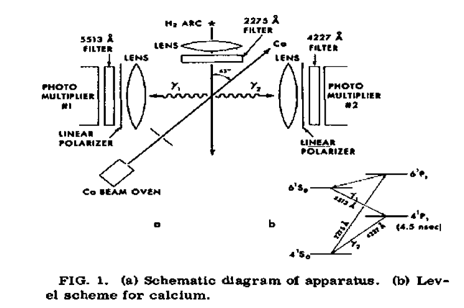
The first such experiment is presented in [6]. The authors measured photons from the cascade 6 in calcium. To understand what correlations between the photon polarizations can be expected, the authors write:
“Since the initial and final atomic states have zero total angular momentum and the same parity, the correlation is expected to be of the form . ”
It means that the wave function of the photons inside the atom can be represented as
| (28) |
where is the vacuum state and are the creation operators for photons with polarizations along or directions. Also, we can rewrite the wave function (28) of the two photons in the form similar to (19),
| (29) |
However since the total electric field of the two photons should be zero, their function is better to write as
| (30) |
where the first letter is related to the photon going to the right, and the second one — to the left. It is clear that we can also write it as a uniform distribution
| (31) |
where and denote particles going to the right and left respectively, similar to (18). Before the decay, the projection of this wave function on two filters oriented along and is
| (32) |
where is the angle between and . After integration we get
| (33) |
which shows that the projection is zero for . Probability of such projections is
| (34) |
Now we will make similar calculations for coincidence counts after the decay.
4.1.1 Derivation of the ratio
After decay the transmission probability of photons through two filters located on left and right and oriented along and respectively is
| (35) |
We immediately see that for or the probability is 3/8, and for it is 1/8. So the predicted ratio is
| (36) |
It is very important to notice that the probability of the coincidence counts with orthogonal filters is not zero. It is only three times less compared to the coincidences with parallel filters. It is also important to note that (35) can be also represented as
| (37) |
so it differs from the result (34) only by a constant!
4.1.2 Experimental results
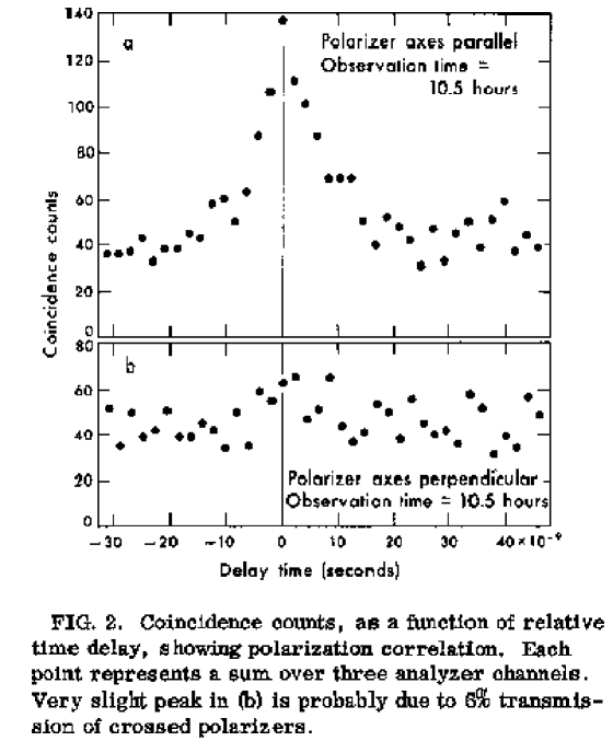
Let’s review the experiment by [6] (Fig. 1). The results of this experiment are demonstrated in fig. 2, where number of counts after parallel and perpendicular analyzers are shown in dependence of delay in coincidence times. We clearly see that the background can be accepted at the level 40 counts, therefore at maximum the coincidence counts with parallel filters is equal to , and the coincidence counts with orthogonal filters is . Thus the measurement precision in this experiment allows for a good agreement with .
However the authors, although absolutely honest, are very reluctant to accept the local realism interpretation. Their conclusion is:
“The results of a 21-h run, shown in Fig. 2. indicate clearly the difference between the coincidence rates for parallel and perpendicular orientations. They are consistent with a correlation of the form . ”
And they attribute the discrepancy at 30% level to 6% transmission of crossed filters, as is documented in the caption of fig. 2. I do not accept such explanation as a proof for action at a distance, while the majority does.
4.2 The experiments by Aspect a.o.
The experiments by Aspect a.o., in particular the first one [5], are commonly accepted as an experimental proof of QM action at a distance. The experiment [5] is very similar to the one described in [6] but instead of the 6 state they excited the state, and they measured the coincidence rates at different angles between the two analyzers. Let’s look at the experimental results, shown in Fig. 3.
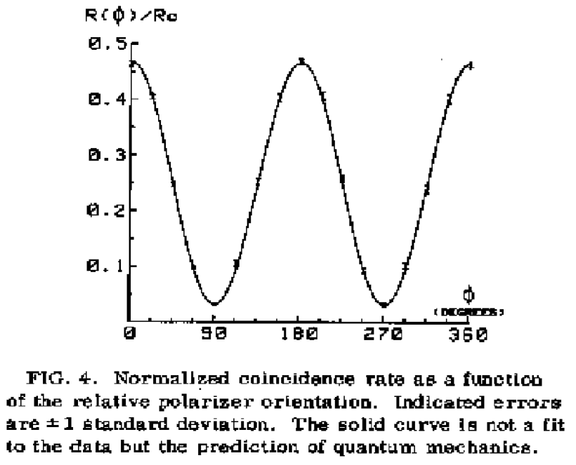
This result can be described as (34) and not as (35), however the difference is only in a constant term 1/8, and in normalization. The normalization is not important as it is more or less arbitrary, but the constant term is crucial. Let’s look how the authors subtracted the constant term:
“Typical coincidence rates without polarizers are 240 coincidences per second in the null delay channel and 90 accidental coincidences per second; for a 100-s counting period we thus obtain 150 true coincidences per second with a standard deviation less than 3 coincidences per second.”
Suppose that not all 90 coincidences are accidental but only 50, while the remaining 40 are not accidental. We then immediately find that at the angle between the polarizers there are 40 coincidence counts, and 115 coincidence counts at (ratio ). In this case there is no contradiction to quantum mechanics, and there is no proof of the spooky action at a distance. Everything is in accordance with our calculations and local realism.
In another experiment by the same authors [7], where the photons are registered by two detectors on each side in order not to lose particles of different polarizations, the background coincidences are also subtracted as accident ones. The decision to consider the counts as accidental, and the number of such counts are cited in the following paragraph,
“Each coincidence window, about 20 ns wide, has been accurately measured. Since they are large compared to the lifetime of the intermediate state of the cascade (5 ns) all true coincidences are registered. We infer the accidental coincidence rates from the corresponding single rates, knowing the width of the windows. This method is valid with our very stable source, and it has been checked by comparing it with the methods of Ref. 5, using delayed coincidence channels and/or a time-to-amplitude converter. By subtracting of these accidental rates (about 10 s-1) from the total rates, we obtain the true coincidence rates (actual values are in the range 0–40 s-1, depending on the orientations).”
From this citation we see again that the subtracted number of coincidences is in the order of value that can also be expected for orthogonal directions of analyzers. Therefore, both experiments [5, 7] must be re-evaluated.
The last experiment [8] is of the “delayed choice” type. I think that the delayed choice experiments do not check anything, since the spooky action at a distance is absent. In conclusion we can say that the results of all cascade experiments are not indisputable enough to reject the local realism.
5 Bell’s inequalities in down-conversion experiments
In the last decade many of experiments that were aimed at proving the violation of Bell’s inequalities were done with spontaneous parametric down-conversion (SPDC) photons. In these experiments, initially polarized photon with frequency splits into two polarized photons with frequencies . The generated photons are thought to be in entangled state, which can be modified with the help of optical devices, and can be used to show the violation of Bell’s inequalities. In the next part of this article we will review three types of such experiments, which use three different approaches to prove the violation — a) photon polarization measurements, b) travel path interference and c) counts statistics. I think that these experiments are well designed, highly resourceful, and can be used to learn a lot about physics of the photon down-conversion, but instead they are narrowly aimed at what appears to be a useless quest — demonstration of the Bell’s inequalities violation.
5.1 Polarization experiments [14].
The schematic of the experiment is shown in Fig. 4. The details of this experiment and the types of the generated entangled states are not included here, because this information is not important in the scope of this work. Instead, we focus on the result presented in Fig. 5. The authors say:
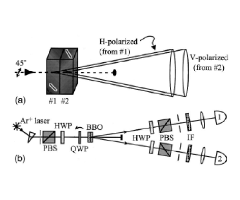
“Figure 5 shows data demonstrating the extremely high degree of polarization entanglement achievable with our source. The state was set to the polarization analyzer in path 1 was set to , and the other was varied by rotating the HWP in path 2.”
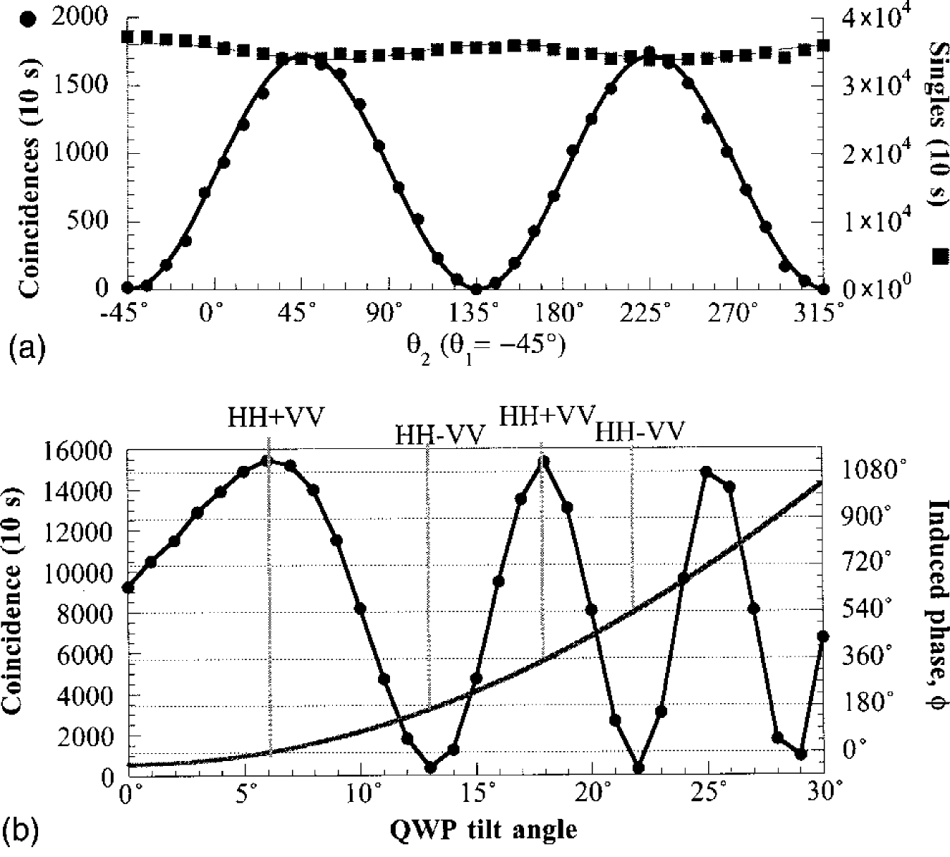
The result in Fig. 5 (upper part) can be easily reproduced without taking into account the entanglements and the action at a distance. Instead, the same data can be acquired if we assume that the photon 1 is polarized at the angle -45∘, and the photon 2 is at the angle +45∘. Furthermore, if both polarizations rotate when the angle of the quarter-wave plate is changed, the lower part of Fig. 5 is also well reproduced. In order to reject such description, the authors should have measured the photons polarizations in the two channels. Such test was not done. The authors limit themselves to noting that the count rate at a single detector does not depend on the orientation of the analyzer (upper part of fig. 5). Notice, however, that the count rate of single counts is at least 20 times higher than the rate of the coincidence counts. No explanation is given to such high level of singles. (See [14].)
In order to reject the above suggestions, the polarization measurements should be done also at coincidence counting. This was not done, therefore the experimental results in [14] are incomplete and cannot be interpreted in favor of the action at a distance. The same conclusion can be drawn about [15] and [16].
5.2 Path interference experiments [17]
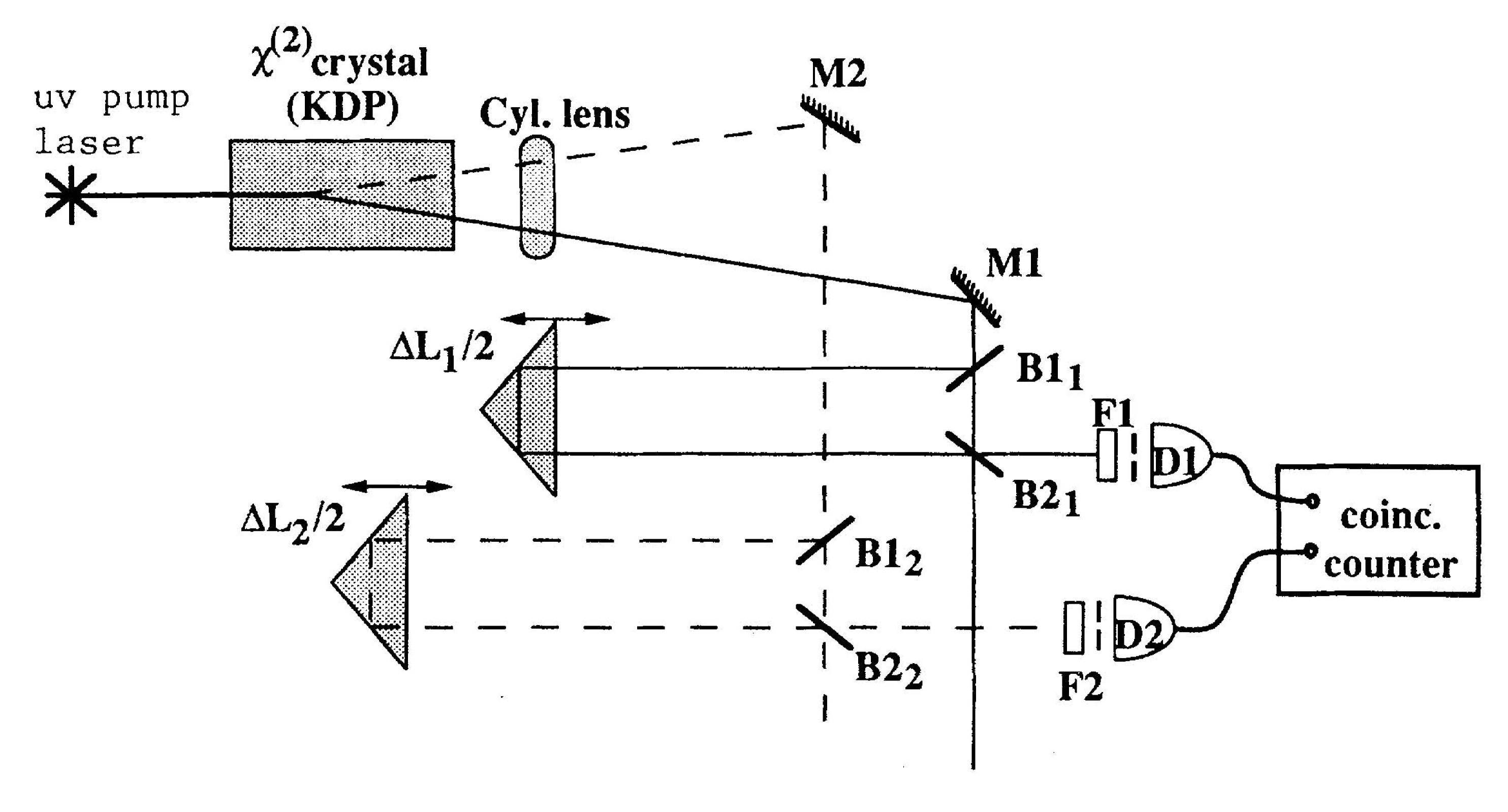
The photons can travel to each detector along two possible paths — a short and a long ones, and the interference of these two paths is measured. It is assumed that the photon travelling to the second detector receives the information about the path chosen by the photon travelling to the first detector, and chooses the same long or short path. If the short path, identical for both detectors, is fixed, and the long one is identically varied, the coincidence count rate periodically changes. This periodic behavior is then used to prove the violation of Bell’s inequalities. However this interference has a very simple alternative explanation, which does not require the action at a distance. When we measure the coincidence counts at time , we count photons created in the crystal at times and , where are the times of flight for photons from the creation point to the detectors along the long and short paths respectively. Since the photons are created by a coherent wave, then the decrease of the count rate at is related to the coherent suppression of the creation of such photons, and not with the interference between the long and short paths. In order to investigate and prove this effect, it is necessary to fix the path difference at one detector and to vary one of the paths to the second one. In this case we could study the interference of the photon down-conversion at three points.
We can conclude that this experiment has nothing to do with the EPR paradox and the action at a distance. The same can be said about experiment [18], where the geometrical change of paths was replaced by time delays.
5.3 Experiments with counting statistics of photons [19]
The schematic of the experiment in [19] (see also [23]) is shown in Fig. 7. In this type of the experiments, both down-converted photons are split at the beam splitter (BS), and each detector therefore counts a combination of both photons.
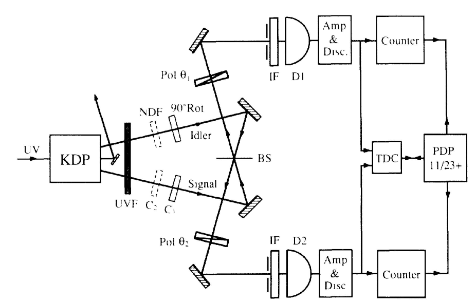
After the beam splitter, the photons A and B are transformed into two mixtures. The mixture goes to the detector 1, and the mixture goes to the detector 2. Because of unitarity of the transformation we must have
The state of the two photons is described now by the product wave function
| (38) |
where the first factor of the direct product is related to the detector 1, and the second factor is related to the detector 2. What is the probability of coincidence counts, if the detectors efficiency is unity? There are two ways to count this probability. The first way, and it is commonly accepted, is
| (39) |
and the second way is
| (40) |
Currently, it is assumed that the interference between photons leads to . On the other hand, the expression for arises from unitarity or in other words from the conservation law for the number of particles. Indeed, the probability for both photons to travel the same path and strike the same detector is
| (41) |
The first term of (41) gives the detection probability of both photons in the first detector only, and the second term gives the registration probability of both photons in the second detector only. According to (40) the total probability of counting both photons in a single detector and at a coincidence in both detectors is
| (42) |
Thus, the unitarity is not violated. In case of (39) the unitarity is violated, because
| (43) |
The unity is achieved only if the last term in the left-hand side is equal to zero, which means that there should be no interference, or no entangled state.
The problem of unitarity is not discussed in the experiments with the photon splitting, therefore the results of these experiments cannot be reliably used to prove the action at a distance.
6 Experiments with neutron interferometer
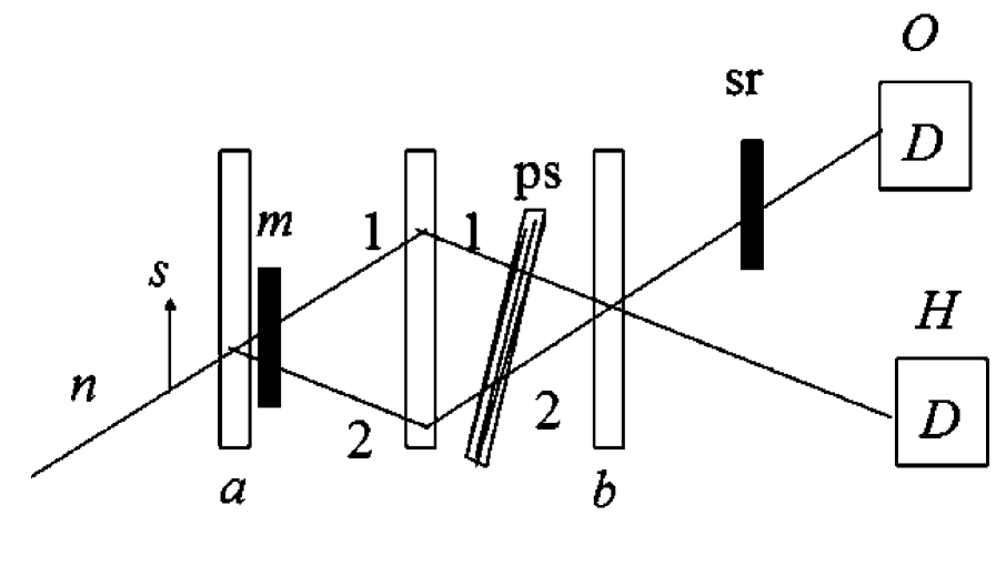
The “disease” of proving the violation of Bell’s inequalities spreads quickly over science. The experiments with neutron interferometer [9, 10] is a good illustration of this statement. In [9, 10] a neutron interferometer (the schematic of the experiment is shown in Fig. 8) is used to create the entangled state for two commuting degrees of freedom of a single particle
| (44) |
The first degree of freedom is the spin, and second degree of freedom is the path that the neutron takes to travel after the first beam splitter. The first term in (44) describes the neutron with the spin state propagating along the path 1 after the beam splitter, and the second term describes the same neutron with the spin state propagating after the beam splitter along the path 2. To achieve the different spin states along two paths, a magnet m with strong inhomogeneous field is placed there after the beam splitter . According to Stern-Gerlach effect the magnet directs neutrons in the state along the path 1, and the neutrons in the state along the path 2.
At the beam splitter the two terms of (44) recombine and give two new beams, one of which (the beam H) propagates toward the detector H and another one (the beam O) propagates toward the detector O. The spin state of the beam O can be represented as
| (45) |
where and are some constants ( is real), and phase can be varied by the phase shifter ps (see fig. 8). The state (45) is a spinor state polarized along some direction :
| (46) |
where is a normalization constant, determined from
| (47) |
The vector is
| (48) |
and .
The experiment [9] uses also a spin rotator sr (see Fig. 8), which rotates the spin around -axis to any desirable angle . In addition, an analyzer is placed after the spin rotator, which transmits neutrons polarized along -axis. Therefore the count rate of the detector O is
| (49) |
We see that the intensity in the detector O oscillates proportionally to , where the phase depends on the phase shift , and the contrast of the oscillations444I regret that in published version [24] there are errors in expressions (49) and (50),
| (50) |
also depends on .
It would be very interesting to check the dependence of on different parameters, however the goal of [9] is different. It is revealed in the first paragraph of the paper [9] (similar description is presented also in [10]):
“The concept of quantum noncontextuality represents a straightforward extension of the classical view: the result of a particular measurement is determined independently of previous (or simultaneous) measurements on any set of mutually commuting observables. Local theories represent a particular circumstance of noncontextuality, in that the result is assumed not to depend on measurements made simultaneously on spatially separated (mutually noninteracting) systems. In order to test noncontextuality, joint measurements of commuting observables that are not necessarily separated in space are required. ”
By proving the violation of Bell-like inequalities and the presence of contextuality the authors want to prove that they deal with quantum phenomenon. This goal is very surprising, because such conclusion is very obvious since the interference is really a quantum phenomenon. The physics becomes like the modern art, which requires a lot of imagination, but not understanding.
7 Conclusion
In this paper I have shown that the non-commutativity of position and momentum operators does not forbid for particles to have well defined positions and momenta simultaneously. Therefore the EPR verdict that QM is not complete is invalid.
I have shown that according to local realism an entangled state of two particles can be considered as a list of possible product states realized in every single trial. To check whether such view is correct, we propose an experiment to measure the ratio of the transmission probabilities through perpendicular and parallel analyzers for two photons after the cascade decay. I have shown that the experiments performed to date do not contradict this view.
I have analyzed several down-conversion experiments and showed that they do not prove the non-locality, but that they should be improved.
I have shown that demonstrating the violation of Bell’s inequalities should not be identified with the proof of QM non-locality. This is especially clear in the case of experiments with neutron interferometer, where everything can be explained from the positions of the local realism.
Finally, I understand that I am embarking on a controversial topic. It is very important for the reader to abandon his/her pre-conceived scepticism, backed by the vast history of this subject, and to understand my arguments in details. Only through constructive debate can the truth be found. The constructive criticism is unfortunately absent from the referees reports, whose main critical points are based on the historical length of the subject, the number of people backing up existing theory and the prominence of the original founders (Einstein and others). While such arguments are valid in presidential elections, they do not apply to science.
8 History of submissions, rejections and discussions with referees
In this article I would like to also include the history of submissions and rejections of this paper to different journals. Throughout this somewhat long process the paper underwent a number of improvements, sometimes according to the the referee reports, sometimes on my own. So, this article looks different from the initial paper submitted to Phys. Rev. A, but the core content remains the same.
8.1 Submission to Phys.Rev.A, section “Fundamental physics”
On March 12, 2007 I submitted this paper to Phys.Rev.A, the Fundamental Physics section. On March 13 I received the submission acknowledgement, and on March 20, only one week after the submission, the article was rejected directly by the editor. His letter is attached below.
Re: AC10282
Dear Dr. Ignatovich,
We are sorry to inform you that your manuscript is not considered suitable for publication in Physical Review A. A strict criterion for acceptance in this journal is that manuscripts must convey new physics. To demonstrate this fact, existing work on the subject must be briefly reviewed and the author(s) must indicate in what way existing theory is insufficient to solve certain specific problems, then it must be shown how the proposed new theory resolves the difficulty. Your paper does not satisfy these requirements, hence we regret that we cannot accept it for publication.
Yours sincerely,
Gordon W.F. Drake Editor Physical Review A Email: pra@ridge.aps.org Fax: 631-591-4141 http://pra.aps.org/
I replied that I do not agree with his decision. The direct rejection unfortunately does not allow for further discussion, so I submitted the article to the Russian journal UFN the day I received the rejection from Phys.Rev. A on March 20.
8.2 Submission to UFN (Uspekhi)
On July 24 I received the email reply with two attached letters. The first letter was the official rejection:
Dear Dr. Ignatovich, your paper and the report of an independent referee were considered. Taking into account critical character of the report we decided to refuse from publication of the paper in UFN. Referee report is attached.
Signed by Deputy Chief Editor, corresponding member of RAS prof. O.V.Rudenko on June 15 2007.
8.2.1 Referee report
The paper criticizes the current approach to analysis of QM paradoxes, based on EPR effect, Bell’s inequalities and Aspect’s experiments. The author claims that the EPR paradox does not exist, and Aspect’s experiments (where it was shown that Bell’s inequalities are violated) prove nothing. The questions raised in the paper are of interest and they are actively discussed in literature. However formulation and discussion of these questions in the submitted article looks not sufficiently complete, and deduced conclusions are not well based. The main defects of the author’s approach are the following.
-
1.
The logic of proofs is not very clear, which is very important for this matter.
-
2.
There are no detailed comparisons of author’s conclusions with the current point of view and no analysis of differences is given. Situation is especially complicated by the formalism which the author uses for derivation of specific equations. His formalism is more complicated than the usual one. So the proofs become non transparent. For instance, the relation (25), derived by the author contradicts to currently accepted Eq. (20), however the author does not discuss sufficiently clear the reasons of such difference. The nontransparent logic of presentation and absence of legible and multifold comparisons with conclusions with current ones makes the author’s results dubious. There is one essential defect in the author’s logic, which seems becomes the reason of all the misunderstandings. He uses a different, unusual definition of the key notion for the given problem, the notion of the “state” in which the observable has a certain value. The author writes ”We shall show that paradox appears only because of definition of ”precise values” of physical quantities as eigenvalues of their operators. We shall show that it is necessary to define them as expectation values, then noncommutativity of operators does not forbid for Q and p to have precise values simultaneously, and the EPR paradox disappears”. However the current definition of “certain values” based on eigen values has an evident ground (the result of measurement in that case is uniquely predicted), and in the case of expectation value it is unpredictable. It is clear that this key notion needs discussion and proof. Their absence invalidates all the conclusions of the article. Because of it the submitted paper cannot be published in UFN.
8.2.2 My reply
I replied to the editors that the referee report was not interesting, that my paper was submitted to ZhETF where the referee reply was much more interesting, and that I will not continue the discussion with the referee of UFN.
8.3 Submission to ZhETF (JETP)
After my submission to UFN, I did not receive any acknowledgement, therefore I submitted the paper to the Russian journal ZhETF (JETP) on March 27. The next day I received the acknowledgement, and on April 2nd I received a letter that my manuscript was accepted for refereing. The referee report was mailed to me on May 24. At that time my paper did not contain discussion of down-conversion experiments.
8.3.1 Referee report (translated from Russian)
I believe that the paper by Dr. Ignatovich should not be published in ZhETF for the following reasons.
-
1.
There are many different publications in the scientific and popular literature devoted to the studies of the EPR “paradox”. It is well known that the resolution of the “paradox” was already given by N.Bohr [20],
-
2.
To my opinion, the best methodical description of the EPR paradox is presented in the book
2. A.Sudbery. Quantum mechanics and physics of elementary particles (Chapter 5, section 5.3)
In that respect it is surprising that V.K.Ignatovich still thinks that the state of a subsystem (single particle) after a decay is described by a wave function instead of the density matrix (see Eq-s (19) and (8)).
-
3.
The problem of Bell’s inequalities, which quantitatively shows the difference between the classical and quantum description of the world, is indeed a very exciting problem to any physicist. To date, numerous experimental and theoretical papers were devoted to the derivation of these inequalities for a wide set of physical systems including those with high dimensionality, e.g. Hilbert space.
I recommend [Dr. Ignatovich] to read the paper by
3. N.V.Evdokimov et all UFN (Russian journal Uspekhi) v.166, p. 91-107 (1997); especially the Introduction, where methodical aspects of the problem are considered.
-
4.
It appears that the arguments of V.K.Ignatovich in his views about the experiments on Bell’s inequalities are highly biased. My opinion is based on the fact that [Dr. Ignatovich’s] “proof” of the relation (36) is based on the experiments performed with large uncertainties. See for example the experiments with the two-photon cascade decay of atoms. Due to the high complexity of the setup and the measurement technique at the time, the measurement precision is not too high. At the same time, numerous experiments with the parametric down-conversion of photons were performed in the past ten years. Relative simplicity of these experiments and the availability of the efficient photon counters and driving electronics allowed to significantly increase the measurement precision. I point out just a few of [these experiments] [17, 18, 19, 15, 14].
In the modern experiments with quantum optics, the coincidence counting techniques utilize time windows below 1ns, thus making the number of the accidental coincidence counts negligibly small. For example, the number of the accidental coincidences in [14] was less than 1Hz, while the true coincidence count was 1.5 kHz in the maximum of the interference pattern.
One can find a large number of such examples. All these experiments prove the validity of the orthodox version of the Bell’s inequality. Why wouldn’t V.K.Ignatovich apply his “theory” [sic] to these experiments?
-
5.
Unfortunately I am not a specialist in the neutron interferometry. However I can assume that in this case, too, the adequacy of the author’s “theory” is based on the experiments conducted with not high enough precision, thus the presence of the background allows [the author] to interpreted the results in his favor. I consider such approach to be one sided. I think it is inappropriate to publish such arguments, which in addition are presented in a highly ambitious way (”:experiments are shown to prove nothing”), in a journal of such level as ZhETF.
8.3.2 My reply to the referee
-
1.
Bohr [20] in his article did not resolve the paradox. Instead he proposed
“a simple experimental arrangement, comprising a rigid diaphragm with two parallel slits, which are very narrow compared with their separation, and through each of which one particle with given initial momentum passes independently of the other.”
In this arrangement either both particles positions or momenta are measured.
“In fact to measure the position of one of the particles can mean nothing else than to establish a correlation between its behavior and some instrument rigidly fixed to the support which defines the space frame of reference. Under the experimental conditions described such a measurement will therefore also provide us with the knowledge of the location, otherwise completely unknown, of the diaphragm with respect to this space frame when the particles passed through the slits.”
From his explanations it follows that after installation of a diaphragm rigidly fixed to support to measure position of a particle in my room, I immediately establish the space frame of reference and geometry in the whole world, and all the other scientists are now able to measure only positions of their particles and no one can measure momenta, because it is not known whether the measured particles were not interacting some time ago. Shortly: there is nothing in this paper about paradox but philosophy about complementarity.
-
2.
Presentation of the EPR paradox in the book [21] is the standard one. I found nothing about density matrix in the section pointed out by referee. The states of free single particles and entangled states of two particles are always pure ones. The density matrix appears when one describes a beam of particles, where averaging over some parameters is necessary. So I do not see any error in using pure states instead of density matrix. More over, I found no density matrix in all the papers describing down conversion experiments, which I had read.
-
3.
With a great pleasure and surprise I had read the paper [22], and I had found there the following. Let’s look page 93 at the left555The following text is translated by me. Readers are advised to look English edition of this paper
“There rises a natural question: how, for instance, position of a switcher at A can affect the color of lamp, which will be switched on at B?”
and further at the right:
“Frequently in the context of quantum experiments the answer is this is a result of the quantum non locality. It means presumably that there is some mysterious super light influence of an apparatus in A on the event in B and vice versa.”
I have to say that it is just this meaning is supposed in quantum mechanics. The word “presumably” shows that the paper has no relation to the EPR paradox. The following paragraph on the same page proves it:
“observation of correlations means transfer of information (protocols of tests with fixation of current number of trial) from A and B to a third observer C via ordinary communication channels.”
It is great! Therefore when a molecule decays at C into two atoms with spin 1/2 two parallel analyzers at A and B will not count in coincidence, because they sent in advance an information to the molecule, and it will decay to atoms with their spins exactly along the direction of the analyzers! Therefore the Wheeler’s proposal to deceive the molecule by switching randomly direction of one of analyzers after the decay is very important! However the God is great! He knows the maleficence of experimentalists and he knows construction of generators of random numbers, so he foresees the outcome of the generator and communicate it to the molecule! How great becomes the physics. It should be taught in churches, — not in the Universities!
-
4.
Thanks to referee for this remark. I thought that dethronement of the experiments by A.Aspect et all is sufficiently important, because till now they are considered as a main experimental proof of the quantum non locality. For example, let’s look at the paper [4]. In the introduction we read
“The concept of entanglement has been thought to be the heart of quantum mechanics. The seminal experiment by Aspect et al. [5] has proved the ”spooky” nonlocal action of quantum mechanics by observing violation of Bell inequality with entangled photon pairs.”
However the referee is right. It is necessary to review at least some (there is a flood of them in literature) experiments on parametric down conversion of photons and to show that they do not prove the action at a distance. Measurement of violation of Bell’s inequalities, which is equivalent to sum
is wasting of time and resources, and it has nothing to do with physics. The experiments themselves are interesting and genuine and they can be used to study physics of down conversion, but instead of it the authors are satisfied to calculate , because it rises their work to the rank of “basic” research!
I sent my replies without the new version of the manuscript on August 1, and received only a reply that my letter was forwarded to the referee. On September 6 I sent a new version of my manuscript, which contained the discussions of the down-conversion experiments. On October 29 I sent an updated version of my manuscript. On the same day I received the final rejection and the second referee report. I had no opportunity to continue the discussion, but I wanted to comment on his report. I added my comments in italic below.
8.3.3 The second referee report
The author discusses the foundations of quantum mechanics. Specifically, he analyzes the famous Einstein-Podolsky-Rosen paradox in the original and Bohm formulations, discusses briefly the Bell inequalities. He suggests new formulations of basic principles of quantum mechanics, which in his view resolve the problems, and analyzes some experiments in order to demonstrate that they in fact do not support the standard view but rather are inconclusive or support his view. I do not find the paper suitable for publication in JETP since the problems discussed are not considered as such any more; furthermore, the author suggests to replace the basic concepts of quantum mechanics to “resolve” the problems — this can hardly be viewed as a resolution. I discuss this in more detail below. Further, the author does not properly describe the context of this work and does not define precisely, which physics problems are being solved; this makes the manuscript hard to follow.
The referee basically says that the debate is closed for the EPR paradox, thus no more articles should be published. I am somewhat at a loss on how to comment on this statement, except that I disagree with the referee’s opinion.
Through the paper he stresses and “illustrates” that the uncertainty principle is invalid and does not make sense.
This argument is not true. I claim that the uncertainty principle is valid, but it does not have the crucial role that it is given in quantum mechanics.
Instead, he suggests that, for instance, the coordinate and momentum can simultaneously have well definite values (no fluctuation)
There are indeed no fluctuations, but there is dispersion. For example, the Gaussian wave packet has precisely defined position, but it also has width, which is the dispersion. It was von Neumann, who proved that there are no dispersion free states for position and momentum operators.
To achieve this, he proposes (in the context of the work by Einstein, Podolsky and Rosen) in order “to avoid paradox”, to “reject the definition” of the concept of “an operator A having some value with certainty (without fluctuations)”: while this happens only when the system is in eigenstate of A with the eigenvalue , he suggests that the operator always has a certain value , which we usually refer to as the average value. In this sense, he throws away a significant notion of the uncertainty principle, and merely observes that every operator has some average value in any state. Similarly, he “shows” that all components of a spin-half can simultaneously have well defined values, without fluctuations; this is again achieved by replacing the notion of an eigenvalue by that of an average. He disregards the fact that the fluctuations, , are vanishing only in eigenstates of A.
If this referee happened to review the book of von Neumann, the book would never got accepted for publication. As for spin half particle: suppose that the particle is polarized along a vector . The average (expectation value in my opinion) of the Pauli matrix (operator) is . What referee calls fluctuation is
It is a fluctuation by definition, but not by physics. It means that the actual value of the component depends on the choice of the coordinate axis and nothing else. Moreover, the operator is just an operator, for which the value can also be found as an expectation value.
I should stress that the ”EPR paradox”, and its reformulation due to Bohm, are not considered as paradoxes, but are used in the modern literature to illustrate the non-local nature of quantum mechanics and the notion of entanglement, as well as to show how quantum mechanics contradicts the classical intuition. They also demonstrate that, unlike the classical physics, the measurement (of one particle of the two) influence the “state” of the other particle (or rather the result of subsequent measurements on this other particle) provided the particles are in an entangled state. In this sense it is impossible to say that, say, one spin in a singlet pair has a well defined direction, which one could try to “guess” (as the author suggests).
The non-local nature of quantum mechanics is direct consequence of the paradox. The action at a distance is introduced to resolve the paradox and to avoid conclusion that QM is not a complete theory. But if there was no paradox to start with, the notion of action at a distance would never appear. Resolving the paradox in an alternative way casts doubt on the accepted notion of entanglement. While QM challenges the classical intuition, it should not be the source of miracles. We of course can debate the issue for very long time, but why not just attempt to measure the coincidence counts of two photons in Aspect’s a.o. experiments with two perpendicular analyzers?
In the discussion and derivations the author implicitly (or explicitly) replaces the rules of quantum mechanics to derive “new results” or “ resolve problems”. For example, in eqs. (23) and (35) he adds probabilities rather than amplitudes, which one can also describe by saying that he assumes that the state (the spin singlet or the state of two photons after decay) is a mixture, rather than a superposition, of “classical” states, where in each constituent state in the superposition one spin has direction , and the other — ( being an arbitrary unit vector). Using these “rules” he derives new expressions for the probabilities of detection.
This statement is again not true. I do not use the mixture of states. I use pure product states, but I average the final probabilities obtained with these pure states over the initial states after decay. I basically follow what we always do in scattering theory. We obtain scattering amplitude, square it modulo then sum over the final states and average over the initial ones. It does not mean that we use mixtures.
Acknowledgement
I greatly appreciate very interesting discussions with my son F.V.Ignatovich and his advices. They helped me very much to improve the paper. I also very grateful to editorial board of Concepts of Physics, and especially to Executive Editor Edward Kapuscik for constructive attitude to my works.
References
- [1] A. Einstein, B. Podolsky, and N. Rosen. Physical Review. May 15, 1935, v47, pp 777-780.
- [2] D.Bohm and Y.Aharonov.“Discussion of experimental proof for the paradox Einstein, Rosen, and Podolsky,” Phys. Rev. 108 (1957) 1070.
- [3] J.S.Bell. Physics 1 (1964) 195; J.S.Bell. “Speakable and unspeakable in quantum mechanics.” Cambridge University press, 2004, p. 14.
- [4] Masahito Hayashi et all, Hypothesis testing for an entangled state produced by spontaneous parametric down-conversion, Phys. Rev. A 74, 062321 (2006)
- [5] A.Aspect, P.Grangier, G.Roger, Experimental tests of realistic local theories via Bell’s theorem. Phys. Rev. Let. V.47, (1981) P. 460.
- [6] C.A.Kocher, E.D.Commins, “Polarization correlation of photons emitted in an atomic cascade.” PRL 18 (1967) 575-577.
- [7] A.Aspect, P.Grangier, G.Roger, Experimental Realisation of Einstein-Podolskii-Rosen-Bohm Gedankenexperiment: A new violation of Bell’s inequalities. Phys. Rev. Let. V. 49 (1982) 91.
- [8] A.Aspect, J.Dalibard, G.Roger, Experimental test of Bell’s inequalities, using time-varying analyzers. Phys. Rev. Let. V. 49 (1982) P. 1804.
- [9] Y.Hasegawa, R.Loidi, G.Badurek, M.Baron, H.Rauch,Violation of a Bell-like inequality in single-neutron interferometry. Nature, V.425 (2003) P. 45-48.
- [10] Y.Hasegawa, R.Loidi, G.Badurek, M.Baron, H.Rauch,Quantum contextuality in neutron interferometer experiment. Physica B V. 385-386, Part II, (11 November 2006) P. 1377.
- [11] J. von Neumann, Mathematical Foundations of Quantum Mechanics. (Princeton University Press, Princrton, New Jersey, 1955) Ch.IV, sec.1 and 2.
- [12] J.Albertson, Am. J. Phys. 29 (1961) 478.
- [13] V.K.Ignatovich ”On uncertainty relations and interference in quantum and classical mechanics” Concepts of Physics, V..III, p. 11, 2006.
- [14] P.G.Kwiat, E.Waks, A.G.White, I.Appelbaum, and P.H.Eberhard, Ultrabright Source of Polarization Entangled Photons. Phys.Rev.A, 60, R773-R776 (1999).
- [15] 7. P.G.Kwiat, K.Mattle, H.Weinfurter, A.Zeilinger, A.V.Sergienko, Y.H.Shih, New High-Intensity Source of Polarization-Entangled Photon Pairs. Phys.Rev.Lett., 75, 4337-4341 (1995).
- [16] P.G.Kwiat et all, Phys.Rev.A, 66, 013801 (2002).
- [17] P.G.Kwiat, A. M. Steinberg, and R. Y. Chiao, “High-Visibility Interference in a Bell-Inequality Experiment for Energy and Time.” Phys. Rev. A, 47, R2472-R2475 (1993).
- [18] T.B.Pittman, Y.H.Shih, A.V.Sergienko, and M.H.Rubin, “Experimental Test of Bell’s Inequalities Based on Spin and Space-Time Variables.” Phys.Rev.A, 51, 3495-3498 (1995).
- [19] Z.Y.Ou and L.Mandel, Violation of Bell’s Inequality and Classical Probability in a Two-Photon Correlation Experiment. Phys.Rev.Lett., 61, 50-53 (1994).
- [20] N.Bohr, Can Quantum Mechanical Description of Physical Reality Be Considered Complete? Phys.Rev., 48, 696-702 (1935). We develop and
- [21] A.Sudbery. Quantum Mechanics and the Particles of Nature: An Outline for Mathematicians. Cambridge University Press, London, 1986.
- [22] N.V.Evdokimov et all UFN (Russian journal Uspekhi) v.166, p. 91-107 (1997)
- [23] Giovanni Di Giuseppe, Mete Atatüre, Matthew D. Shaw, Alexander V. Sergienko, Bahaa E. A. Saleh, and Malvin C. Teich, “Entangled-photon generation from parametric down-conversion in media with inhomogeneous nonlinearity.” Phys. Rev. A 66, 013801 (2002).
- [24] V.K.Ignatovich, ON EPR PARADOX, BELL’S INEQUALITIES AND EXPERIMENTS THAT PROVE NOTHING, Concepts of Physics, the old and new, v. 5, No 2, pp. 227-272, 2008.