Quantum phases of interacting phonons in ion traps

Abstract

The vibrations of a chain of trapped ions can be considered, under suitable experimental conditions, as an ensemble of interacting phonons, whose quantum dynamics is governed by a Bose–Hubbard Hamiltonian. In this work we study the quantum phases which appear in this system, and show that thermodynamical properties, such as critical parameters and critical exponents, can be measured in experiments with a limited number of ions. Besides that, interacting phonons in trapped ions offer us the possibility to access regimes which are difficult to study with ultracold bosons in optical lattices, like models with attractive or site–dependent phonon-phonon interactions.

I Introduction

The interplay between atomic and many–body physics has proved to be an exciting research field in the last years. Experiments in atomic physics offer us the possibility to find experimental realizations of theoretical models which were first proposed in the context of solid state physics. Many of these models are the key to understanding a variety of phenomena in real materials such as quantum magnetism or superconductivity. For example cold bosonic atoms in optical lattices are a realization of the Bose–Hubbard Model (BHM) in a clean experimental setup, where one can tune the value of interactions and observe quantum phase transitions in a controlled way mott . The main handicap of experiments with optical lattices is the fact that atoms are separated by optical wavelengths, and thus single particle addressing with optical means is severely limited by diffraction effects.

Trapped ions are also an experimental system with potential applications to the quantum simulation of many–body problems PorrasCirac.spin ; PorrasCirac.phonon ; DengPorrasCirac.spin ; Milburn ; PorrasCirac.2D . It has the advantage that internal electronic or vibrational quantum states can be measured at the single particle level Leibfried.review ; Meekhof , since the distance between ions is large enough to address them individually by optical means. In particular, we have recently shown that the vibrational modes of a chain of trapped ions under suitable experimental conditions follow the quantum dynamics of a BHM PorrasCirac.phonon . The interaction between phonons is induced by the anharmonicities of an optical potential, which can be created by an off–resonant standing–wave.

In this work we present a theoretical study of interacting phonons in trapped ions, and show the following results: (i) The quantum phase transition between a superfluid and a Mott insulator phase can be induced and observed in this system. (ii) Even though finite size–effects are important due to the finite length of the ion chain, properties corresponding to the thermodynamical limit can be accessed in experiments with a limited number of ions. These include critical exponents of correlation functions, and critical values of parameters in the Hamiltonian. (iii) The ability to control phonon–phonon interactions allows us to realize models of interacting bosons which are difficult to reproduce in other experimental setups, like for example, BHM’s with negative interactions, as well as models with site dependent interactions.

The structure of the paper is the following. In section II we derive the Bose–Hubbard model for phonons in a chain of trapped ions, in the presence of the anharmonicities induced by an optical dipole potential. The DMRG algorithm that we have used to study numerically this problem is summarized in section III. In sections IV and V, we study the quantum phases which correspond to repulsive and attractive phonon–phonon interactions, respectively. Section VI is devoted to the case of a Bose–Hubbard model with site–dependent interactions. Finally in the last section we summarize our results and conclusions.

II Bose-Hubbard model of phonons in ion traps

In this section we show that under certain experimental conditions, the dynamics of the vibrational modes of a chain of ions satisfies the Bose-Hubbard model of interacting phonons in a lattice PorrasCirac.phonon . Phonon number conservation is ensured whenever vibrational energies are much higher than other energy scales in the system. In this limit, physical processes which involve creation or destruction of a phonon do not conserve particle number and are suppressed in much the same way as processes which do not conserve the number of electrons or atoms in low–energy physics.

II.1 Hamiltonian in the harmonic and phonon conserving approximation

Let us start by writing the Hamiltonian that describes a chain of ions in a linear trap:

$$H_{0}=\sum_{i=1}^{N}\frac{{\vec{P}}_{i}^{2}}{2m}+V_{\textmd{T}}+\sum_{\begin{subarray}{c}i,j=1\\ (i>j)\end{subarray}}^{N}\frac{e^{2}}{|\vec{R_{i}}-\vec{R_{j}}|}.$$ (1)

$N$ is the number of ions, and $m$ is their mass. $\vec{P}_{j}$ and $\vec{R}_{j}$ are the momenta and the absolute positions of the ions, respectively. $V_{\textmd{T}}$ is the trapping potential, which determines the ions’ equilibrium positions. In this work we deal with two different situations. On one hand we consider the case of ions in a linear Paul trap, where they are confined by an overall trapping potential:

$$V_{\textmd{T}}=\frac{1}{2}m\sum_{i=1}^{N}\sum_{\alpha=x,y,z}\omega_{\alpha}^{2}R^{2}_{i,\alpha},$$ (2)

where $\omega_{\alpha}$ are the trapping frequencies in each spatial direction. On the other hand, we consider ions confined by an array of separate microtraps:

$$V_{\textmd{T}}=\frac{1}{2}m\sum_{i=1}^{N}\sum_{\alpha=x,y,z}\omega^{2}_{\alpha}\left(R_{i,\alpha}-\bar{R}_{i,\alpha}\right)^{2},$$ (3)

where $\bar{R}_{j,\alpha}$ are the centers of each microtrap. Note that in (3) we assume that the confinement is strong enough, such that each ion feels only a single microtrap.

The equilibrium positions of the ions are given by the minima of the trapping potential plus the Coulomb repulsion. From now on, we choose the condition $\omega_{z}\gg\omega_{x},\omega_{y}$, such that the ion chain is along the ${\bf z}$ axis, with equilibrium positions given by $z_{i}^{0}$. In the case of a linear Paul trap, described by Eq. (2), the equilibrium positions of the ions have to be calculated numerically. The distance between ions is smaller at the center of the chain. In the case of independent microtraps (Eq. (3)), one can approximate the equilibrium positions by assuming that they correspond to the center of each microtrap: $z_{i}^{0}=\bar{R}_{i,z}$. This fact has strong implications for the phonon quantum dynamics, as we will see below.

In the harmonic approximation, $H_{0}$ is expanded up to second order in the displacements of the ions around the equilibrium positions, and we get a set of independent vibrational modes corresponding to each spatial direction. The phonon number is a conserved quantity if the vibrational energies are the largest energy scale in the system. This condition can be met either in the case of ions in individual microtraps, or in the case of the radial vibrations of ions in a linear trap, because the corresponding trapping frequencies can be increased without destroying the stability of the ion chain. For concreteness we restrict from now on to the case of vibrations in one of the radial directions, say ${\bf x}$, but keep in mind that our results can be applied also to the axial vibrational modes if ions are in individual microtraps.

The Hamiltonian that governs the dynamics of the radial coordinates in the harmonic approximation reads:

$$H_{\textmd{x0}}=\sum_{i=1}^{N}\frac{P^{2}_{i,x}}{2m} + \frac{1}{2}m\omega_{x}^{2}\sum_{i=1}^{N}x_{i}^{2}$$

$$- \frac{1}{2}\sum^{N}_{\begin{subarray}{c}i,j=1\\ (i>j)\end{subarray}}\frac{e^{2}}{|z_{i}^{0}-z_{j}^{0}|^{3}}\left(x_{i}-x_{j}\right)^{2},$$

where $x_{i}$ are the displacements of the ions around the equilibrium positions, that is, simply $x_{i}=R_{i,x}$, and $P_{i,x}$ the corresponding momenta. The second quantized form of this Hamiltonian is (we consider units such that $\hbar=1$):

$$H_{\textmd{x0}}=\sum_{i=1}^{N}\omega_{x,i}a^{\dagger}_{i}a_{i}+\sum^{N}_{\begin{subarray}{c}i,j=1\\ (i>j)\end{subarray}}t_{i,j}\left(a^{\dagger}_{i}+a_{i}\right)\left(a^{\dagger}_{j}+a_{j}\right).$$ (5)

$a_{i}^{\dagger}$ ($a_{i}$) are creation (anihilation) operators for phonons in the radial direction. Harmonic corrections induced by the Coulomb interaction determine the effective trapping frequency, $\omega_{x,i}$ which depends on the ions’ positions, as well as the tunneling amplitudes $t_{i,j}$:

$$\omega_{x,i} = \omega_{x}-\frac{1}{2}\sum_{\begin{subarray}{c}j=1\\ (j\neq i)\end{subarray}}^{N}\frac{e^{2}/(m\omega_{x}^{2})}{|z_{i}^{0}\!-\!z_{j}^{0}|^{3}}\ \hbar\omega_{x},$$ (6)

$$t_{i,j} = \frac{1}{2}\frac{e^{2}/(m\omega_{x}^{2})}{|z_{i}^{0}\!-\!z_{j}^{0}|^{3}}\ \hbar\omega_{x}.$$ (7)

Eq. (6) yields an important result on the properties of phonons in trapped ions: the corrections to the local trapping energy, $\omega_{x,i}$ may depend on the position of the ions, in case the distance between ions changes along the chain. In PorrasCirac.phonon we have shown that in a linear ion trap, ions arrange themselves in a Coulomb chain, such that $\omega_{x,i}$ is an effective harmonic confining potential for the phonons. On the contrary, in the case of an array of ion microtraps, the distances between ions can be considered to be approximately constant, and thus this confining effect does not take place.

Before going any further, let us study under which conditions phonon nonconserving terms of the form ($a_{i}a_{j}$, $a_{i}^{\dagger}a_{j}^{\dagger}$), can be neglected in Eq. (5). We define the parameter:

$$\beta_{x}=e^{2}/(m\omega_{x}^{2}d^{3}_{0}),$$ (8)

where $d_{0}$ is the distance between ions. Since we will be interested in the limit $\beta_{x}\ll 1$, we choose $d_{0}$ to be the minimum distance between ions in the case of a linear Paul trap. Phonon tunneling terms $t_{i,j}$ are of the order of $t$, defined by:

$$t=\beta_{x}\omega_{x}/2.$$ (9)

Since phonon nonconserving terms rotate fast in (5), we can neglect them in a rotating wave approximation if:

$$t/\omega_{x}=\beta_{x}/2\ll 1,$$ (10)

such that Eq. (5) takes the form of tight binding Hamiltonian with hopping terms $t_{i,j}(a_{i}^{\dagger}a_{j}+h.c)$.

In our numerical calculations, we will parametrize the tunneling of phonons between sites by the parameter $t$, which corresponds, due to the definition of $\beta_{x}$, to the highest value of the tunneling along a chain in the case of a linear Paul trap, and to the tunneling between nearest–neighbors in the case of an array of microtraps.

II.2 Phonon–phonon interactions

Anharmonic terms in the vibrational Hamiltonian are interpreted as phonon–phonon interactions, and can be induced by placing the ions at the minimum or maximum of the optical dipole potential created by an off–resonant standing wave along ${\bf x}$:

$$H_{\textmd{sw}}=F\sum_{i=1}^{N}\cos^{2}(kx_{i}+\frac{\pi}{2}\delta).$$ (11)

$F$ is the amplitude of the dipole potential, and $\delta$ determines the position of the ions relative to the standing wave. We define the Lamb–Dicke parameter $\eta=kx_{0}$, where $k$ is the wave–vector of the standing wave lasers, and $x_{0}$ is the ground–state size of the radial trapping potential. The only relevant cases for us are $\delta=0$ (maximum of the optical potential), and $\delta=1$ (minimum). Under the condition $\eta\ll 1$, we can write $H_{\textmd{sw}}$ as a series around $x_{i}=0$. The term that is quadratic in $x_{i}$ in Eq. (11) can be included in the harmonic vibrational Hamiltonian just by redefining the global radial trapping frequency:

$$\omega^{2}_{x}\rightarrow\omega_{x}\left(\omega_{x}-(-)^{\delta}4\eta^{2}F\right).$$ (12)

In the case $\delta=0$, condition $\eta^{2}F\ll\omega_{x}$ has to be fulfilled, such that the radial trapping frequency is not strongly suppressed by the standing wave, and the system remains in the phonon number conserving regime. Under this condition the only relevant term is thus the quartic one:

$$H^{\textmd{(4)}}_{\textmd{sw}}=(-1)^{\delta}\frac{F\eta^{4}}{3}\sum_{j=1}^{N}\left(a_{j}+a_{j}^{\dagger}\right)^{4}.$$ (13)

We can neglect nonconserving phonon terms again under the condition $F\eta^{4}\ll\omega_{x}$. In this way we get, finally, the promised BHM for phonons:

$$H^{\textmd{BHM}}_{\textmd{x}} = \sum^{N}_{\begin{subarray}{c}i,j=1\\ i>j\end{subarray}}t_{i,j}(a^{\dagger}_{i}a_{j}+h.c.)$$ (14)

$$+ \sum^{N}_{i=1}(\omega_{x}+\omega_{x,i})a^{\dagger}_{i}a_{i}+U\sum^{N}_{i=1}a^{\dagger 2}_{i}a^{2}_{i}.$$

The on–site interaction is given by:

$$U=2(-1)^{\delta}F\eta^{4}.$$ (15)

Thus, it is repulsive or attractive depending on whether the ions are placed at a minimum or maximum of the standing-wave, respectively.

III Numerical Method

The Bose–Hubbard Model with tunneling between nearest–neighbors has been thoroughly studied in the past Fisher ; Sachdev . It has recently received considerable attention because it describes experiments with ultracold atoms in optical lattices. In general, we expect the same phenomenology to appear in our problem, such as, for example, a superfluid–Mott insulator quantum phase transition. However, the situation of phonons in ion traps presents a few peculiarities that deserve a careful analysis: the effects of long–range tunneling in (14), finite size effects, as well as the possibility of having attractive interactions.

To handle this many–body problem numerically we use the Density Matrix Renormalization Group method (DMRG) White_DMRG , which has proved to be a quasi–exact method in quantum chains. In particular we use the finite-size algorithm for open boundary conditions. Our problem is defined in the microcanonical ensemble, that is, we find the minimum energy state within the Hilbert subspace with a given number of total phonons $N_{\textmd{ph}}$. For this reason, we have implemented a DMRG code which uses the total phonon number as a good quantum number and projects the problem into the corresponding subspace at each step in the algorithm Schollwoeck_Review .

To keep a finite dimensional Hibert space, we truncate the number of phonons in each ion, and define a maximum value $n_{max}$, which is usually taken to be of the order of $6\langle n\rangle$, with $\langle n\rangle$ the mean phonon number. The number of eigenstates of the reduced density matrix that we keep at each step is always in the range $80-100$.

We have checked the accuracy of our method by comparing our numerical calculations with the exact solution in the case of a system of non–interacting ($U=0$) phonons, where the ground state at zero temperature is a condensate of phonons in the lowest energy vibrational state. We have also compared our numerical results with exact diagonalizations of Eq. (14) with up to $N=5$ ions. In both cases we found agreement between DMRG and the exact results up to machine accuracy $\delta E\sim 10^{-14}$.

The relevant experimental parameters of our phonon-Hubbard model are discussed in the Ref. PorrasCirac.phonon . Typically we could choose the minimum distance between ions $d_{0}=5$ $\mu m$ and $\beta_{x}=2\times 10^{-2}\ll 1$. Then we have $\omega_{z}\approx 177$ kHz and $\omega_{x}\approx 12.5$ MHz for a string of ions with $N=50$. The number of phonons is $N_{ph}=N$ for the superfluid and Mott-insulator phases and $N_{ph}=N/2$ for the Tonks-gas phase. In the end we discuss $N_{ph}=2N$ for a special case with site-dependent interactions. All our calculations are for the ground state, i.e. at zero temperature.

Following the discussion below Eqs. (6, 7), one expects to find significant differences between the cases of phonons in ions trapped in a linear trap (Coulomb chain), and phonons in an array of ion microtraps. Finite size and inhomogeneity effects are indeed much more important in the linear trap case, since harmonic Coulomb corrections induce an effective harmonic trapping for the phonon field. For this reason, we always study these two cases separately, in the different quantum phases that we will explore in what follows.

IV Bose-Hubbard Model with Repulsive interactions: $U>0$

We study first the quantum phases of phonons with $U>0$, and both commensurate and incommensurate total phonon number. In this section we present results for a chain with $N=50$ ions, and total phonon number $N_{\textmd{ph}}=N$ in the commensurate case, or $N_{\textmd{ph}}=N/2$ in the incommensurate case.

The local observables that we consider are the number of phonons at each site, $n_{j}=\langle a^{\dagger}_{j}a_{j}\rangle$, as well as its fluctuations, $\delta n_{j}=\sqrt{\langle n^{2}_{j}\rangle-\langle n_{j}\rangle^{2}}$. Two–point correlation functions have to be defined carefully, to take into account finite size effects, for example, the variations of the density of phonons along the chain. Correlations in the number of phonons are given by:

$$C^{nn}_{i,j}=\langle n_{i}n_{j}\rangle-\langle n_{i}\rangle\langle n_{j}\rangle.$$ (16)

A suitable definition of correlations that are non–diagonal in the phonon number basis is the following one Kollath_correlations :

$$C^{aa}_{i,j}=\frac{\langle a^{\dagger}_{i}a_{j}\rangle}{\sqrt{\langle n_{i}\rangle\langle n_{j}\rangle}},$$ (17)

such that correlations are rescaled by local values of the phonon density. The rescaling is inspired by the decomposition of the phonon field in density and phase operators, $a_{j}=\sqrt{n_{j}}e^{-i\phi_{j}}$, which is the starting point for the Luttinger theory of the weakly interacting bosonic superfluid Haldane ; Gangardt ; Kheruntsyan .

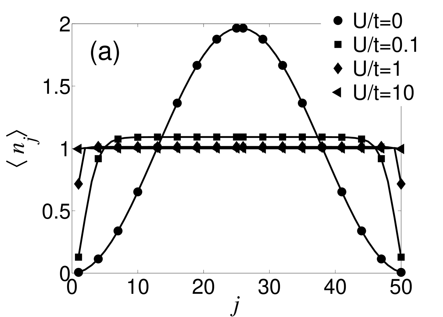
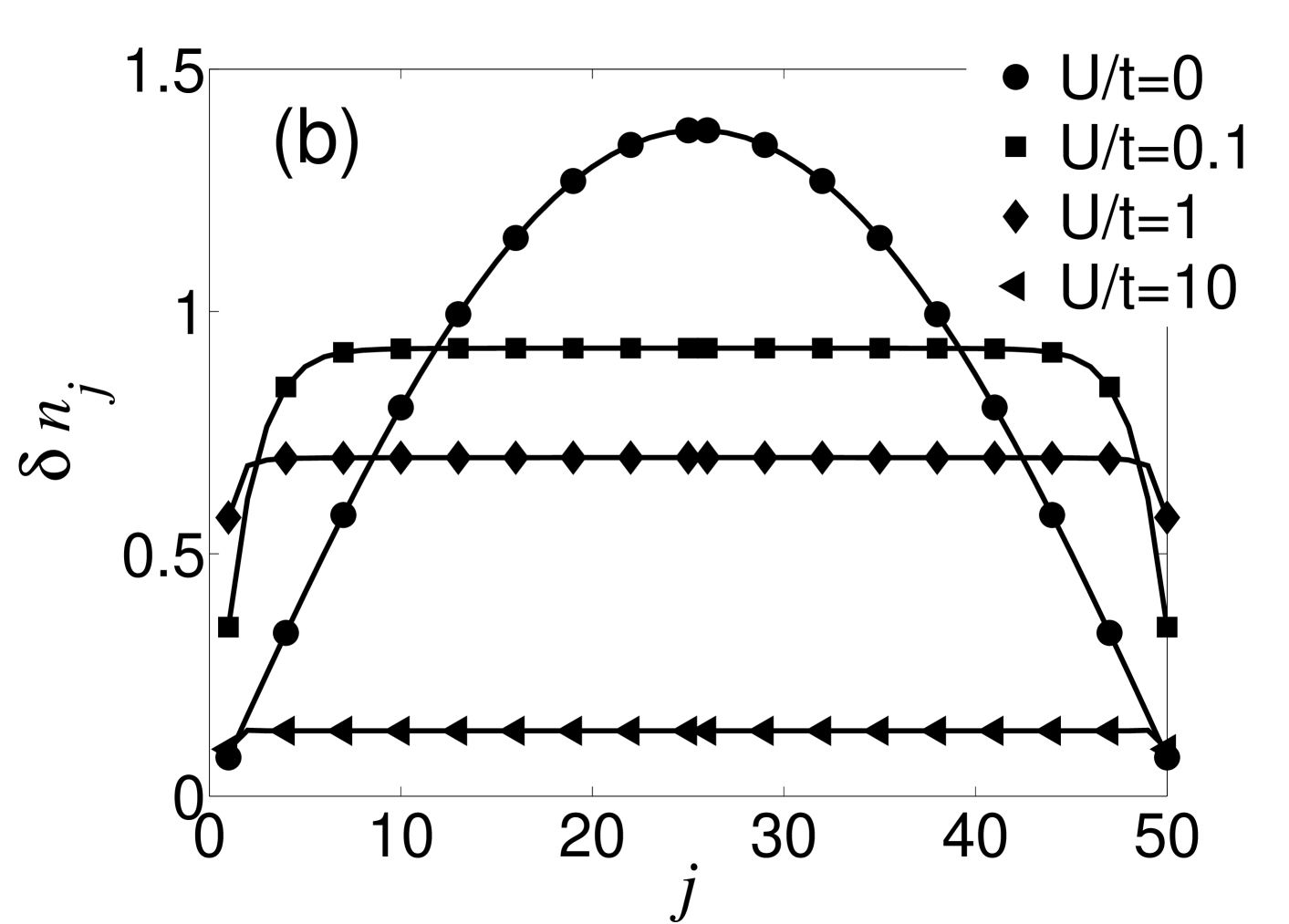
Figure 1: (a) Mean phonon number $\langle n_{j}\rangle$, and (b) fluctuations $\delta n_{j}$, at each ion in the phonon ground state in an array of microtraps. Number of ions $N=50$, and total phonon number $N_{\textmd{ph}}=50$.

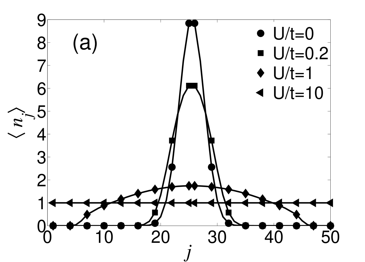
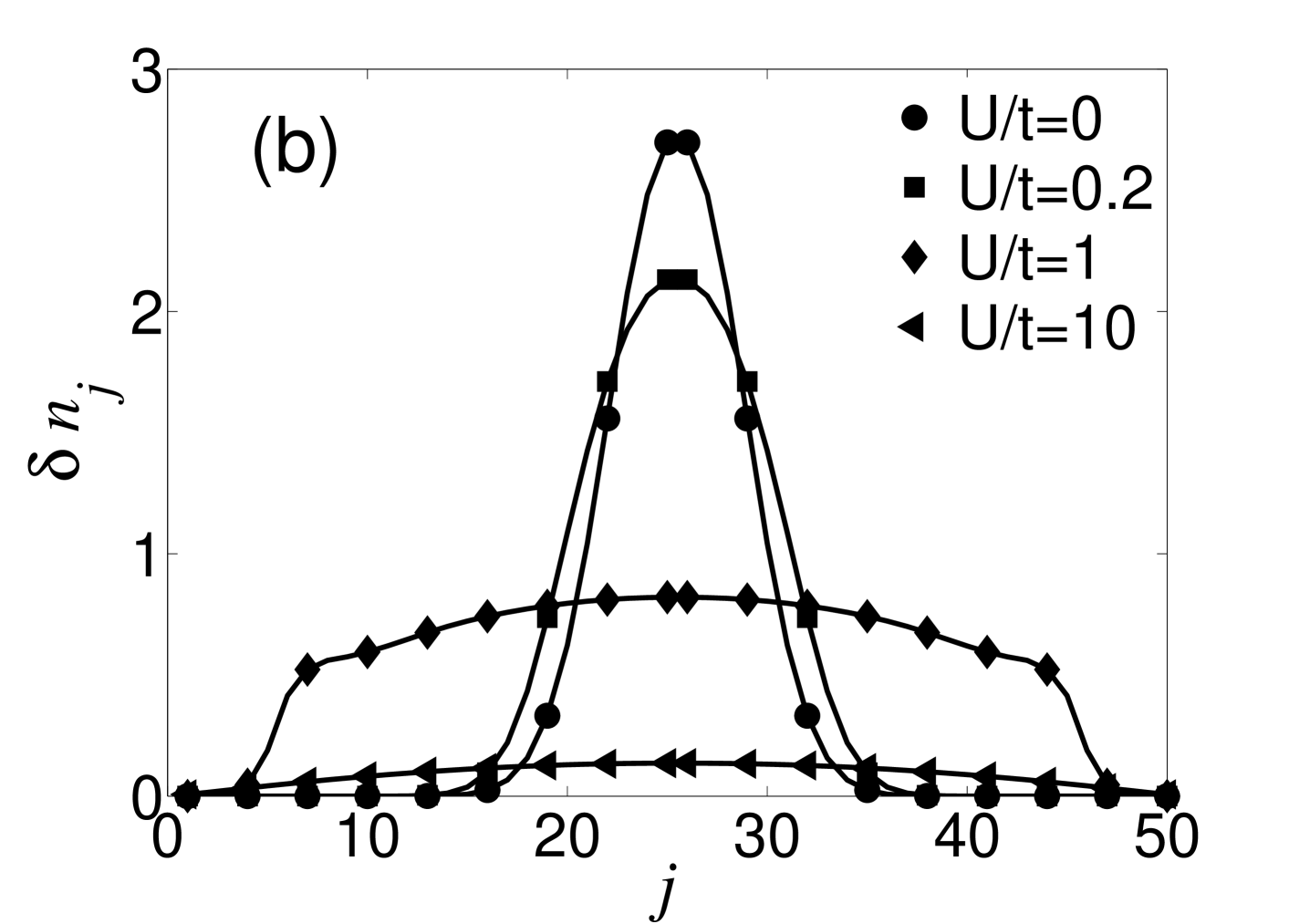
Figure 2: (a) Mean phonon number and (b) fluctuations, at each ion in the phonon ground state in a linear Paul trap. $N=50$, $N_{\textmd{ph}}=50$.

In Figs. 1 and 2, we plot the local density and its fluctuations in the cases of an array of microtraps, and a linear Paul trap, respectively. These figures show a signature of the different phases which can be observed in the model defined by the Hamiltonian (14). Figs. 1(a) and 2(a), in particular, show the variation of the density of phonons along the chain. The evolution of the density profile shows the transition from the phonon superfluid to the Mott–insulating phase. When $t\gg U$, the ground state of the system is a condensate such that all the phonons occupy the lowest energy vibrational mode. In the case of a linear Paul trap, phonons are confined in the center of the chain, due to the effective trapping potential induced by the nonconstant ion–ion distance. At $U\gg t$, the ground state is a phonon Mott insulator with approximately one phonon per site, and no phonon number fluctuations. Note that due to the effective harmonic trapping potential, the Mott phase in the whole chain is reached for lower values of $U$ in the case of the array of microtraps (Fig. 1) than in the linear Paul trap case (Fig. 2).

In the following subsections, we study these two quantum phases separately, paying particular attention to their correlation functions.

IV.1 Superfluid phase

When the tunneling dominates the on–site interactions, the system is in the superfluid phase note1 . The non-interacting ground state is given by a condensate solution in which the $N_{\textmd{ph}}$ phonons are in the lowest vibrational mode:

$$|\psi_{SF}\rangle=\frac{1}{\sqrt{N_{\textmd{ph}}!}}\left(\frac{1}{\sqrt{N}}\sum_{i}{\cal M}^{0}_{i}a^{\dagger}_{i}\right)^{N_{\textmd{ph}}}|0\rangle,$$ (18)

where ${\cal M}^{0}_{i}$ is the wave–function of the lowest energy vibrational mode. Interactions suppress long range order in 1D, even in the weak interacting limit, $U\ll t$, in which Luttinger liquid theory allows us to make predictions on the scaling of correlation functions:

$$C^{aa}_{i,j}\propto|i-j|^{-\alpha},$$

$$C^{nn}_{i,j}\propto|i-j|^{-2},$$ (19)

where $\alpha$ depends on the parameters of the model:

$$\alpha\propto\sqrt{\frac{U/t}{n_{0}}}.$$ (20)

In deriving (19) one has to neglect phonon tunneling beyond nearest–neighbor ions, and assume an homogeneous system Haldane . In the following we will check if Luttinger theory describes also our numerical results in the case of phonons in a chain of trapped ions, by fitting our results to the form (19).

(1) Array of microtraps. We start with the case of the superfluid phase in an array of ion microtraps, see Fig. 3. Correlation functions $C^{aa}_{i,j}$ and $C^{nn}_{i,j}$ decay algebraically in an intermediate range of ion–ion separations, with exponents which satisfy the predictions of Luttinger theory. In particular, the evolution of $\alpha$ in Eq. (19) is well described by the Luttinger liquid scaling law (20), as shown in Fig. 4.

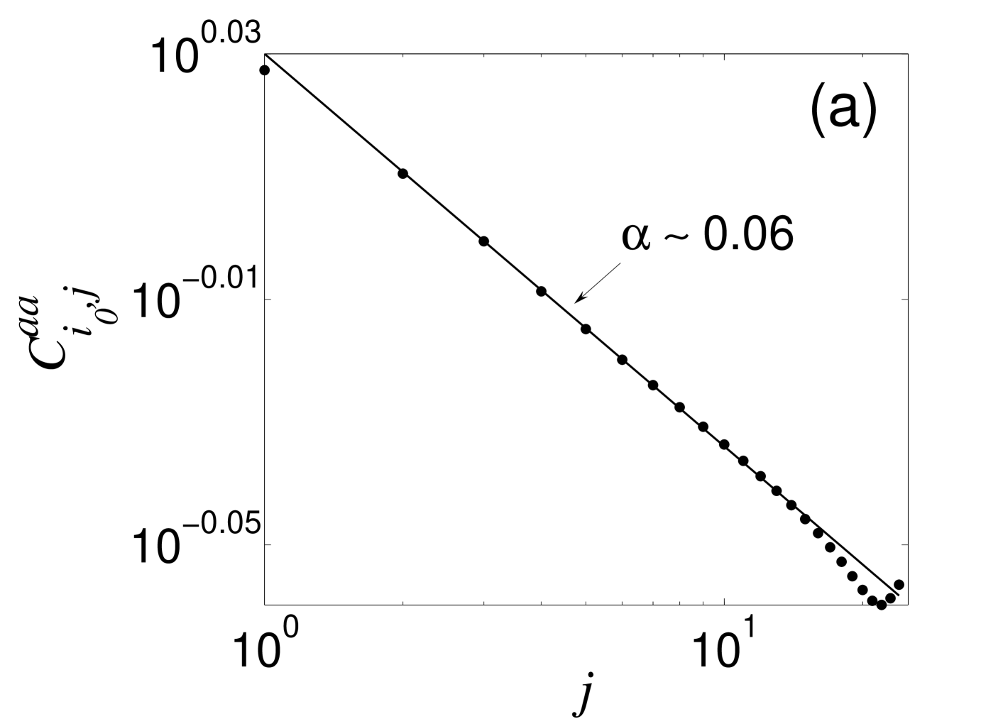
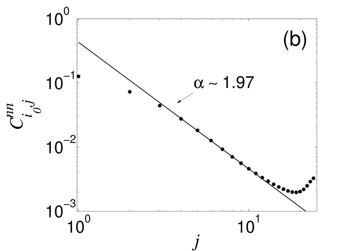
Figure 3: Correlation functions (a) $C^{aa}_{i_{0},j}$ and (b) $C^{nn}_{i_{0},j}$ as a function of coordinate $j$, at the superfluid phase ($U/t=0.1$) in an array of ion microtraps. We choose $i_{0}=26$ (center of the chain), $N=N_{\textmd{ph}}=50$. The dotted and solid lines are numerical results and fittings in the region where the functions show algebraic decay.

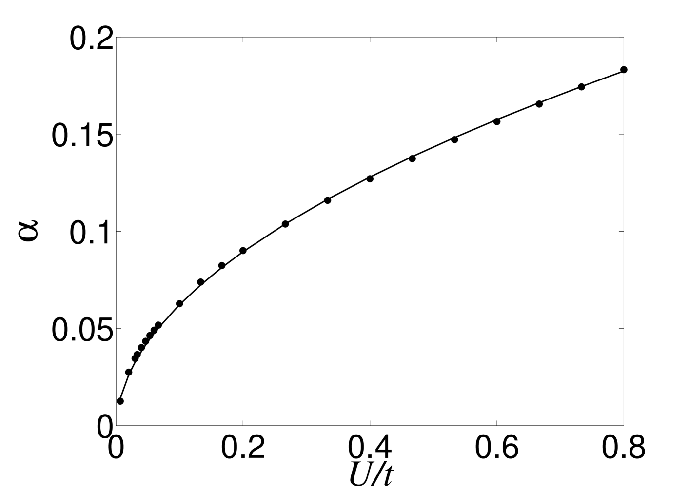
Figure 4: The evolution of the exponent $\alpha$ of $C^{aa}_{i_{0},j}$ as a function of $U/t$ in the regime of superfluid phase, in an array of ion microtraps ($i_{0}=26$, $N=N_{\textmd{ph}}=50$). The dotted line is from numerical data, and the solid line the fitting result from the Luttinger liquid, that is, $\alpha\approx A\sqrt{\frac{U/t}{n_{0}}}$, where the coefficient $A\approx 1.68$.

(2) Linear ion trap. In the case of ions in a linear Paul trap, finite size effects play a more important role, because of the inhomogeneities of the on–site phonon energy. Correlation functions still decay algebraically for short distances in the superfluid regime, but boundary effects spoil this behavior at large separations between ions. In the algebraic regime, exponents are close to those predicted by Luttinger theory in the homogeneous case, see Figs. 5 and 6.

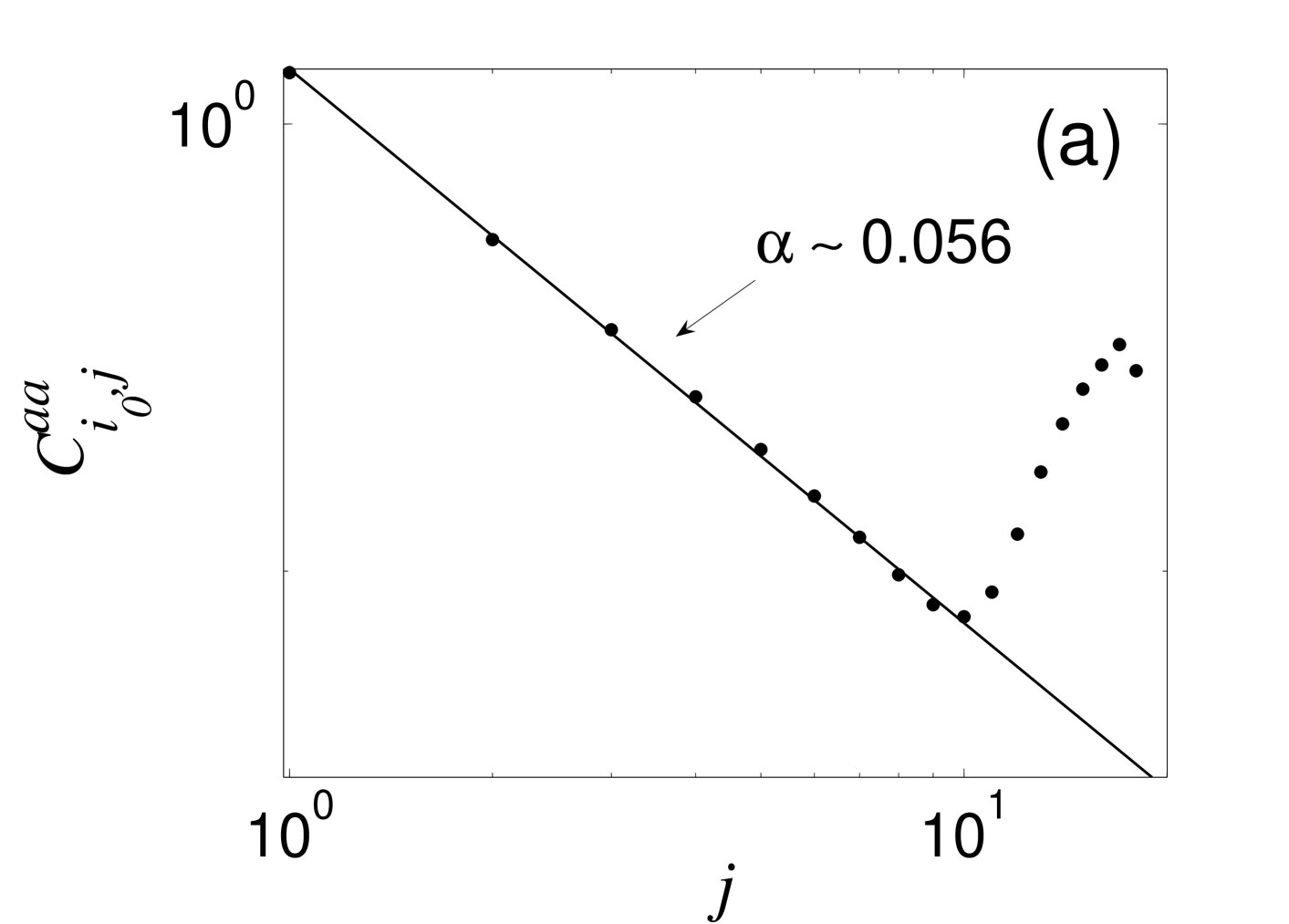
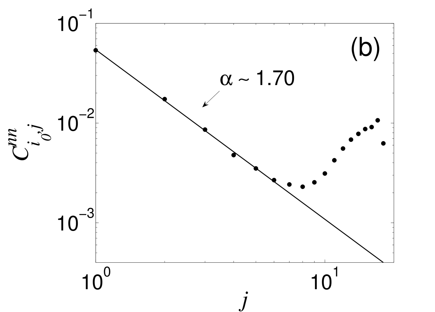
Figure 5: Correlation functions (a) $C^{aa}_{i_{0},j}$ and (b) $C^{nn}_{i_{0},j}$ at the superfluid phase $U/t=0.2$ in a linear Paul trap ($N=N_{\textmd{ph}}=50$). The dotted lines are numerical data, and the solid lines are fittings in the region where the correlations decay algebraically.

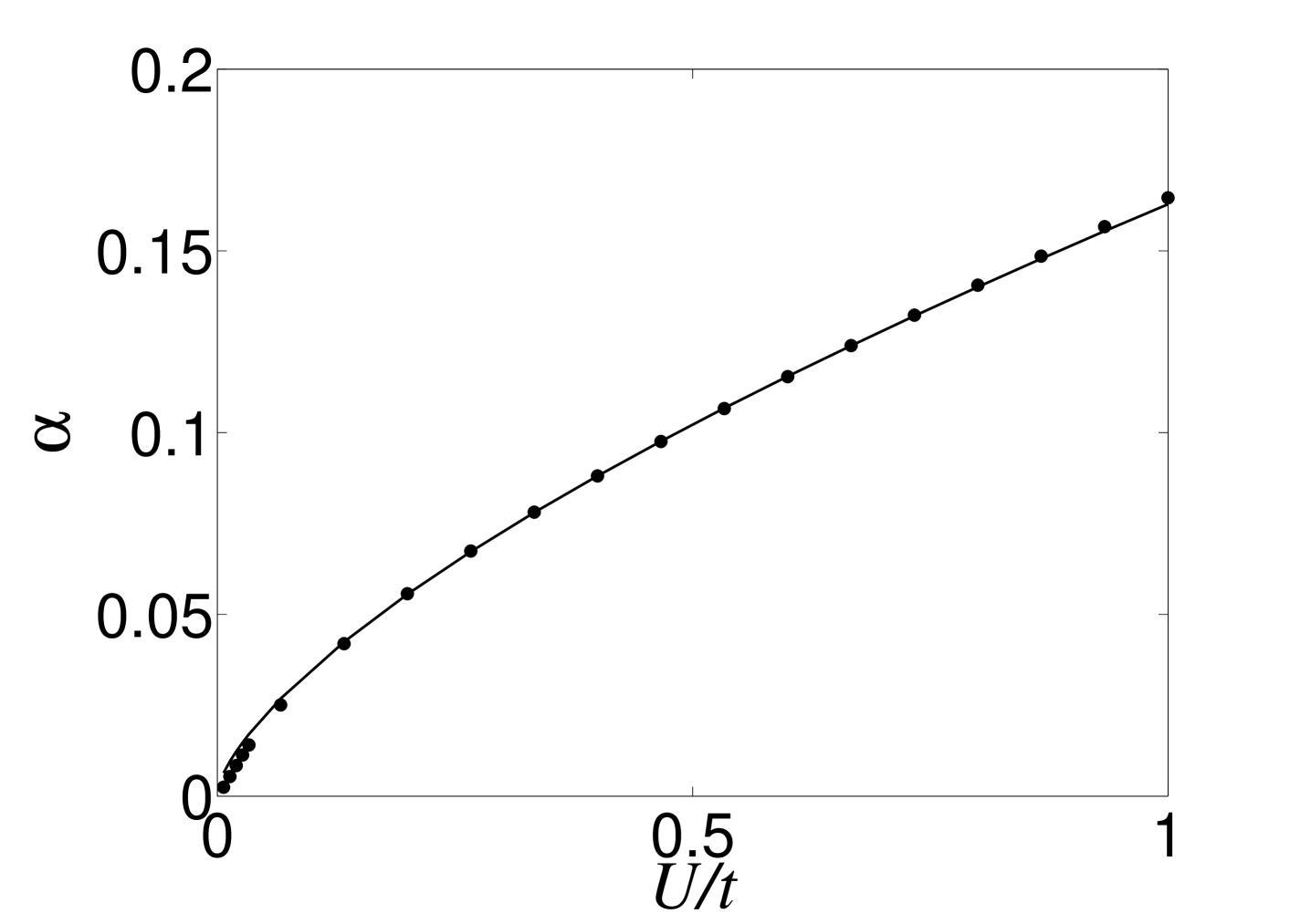
Figure 6: The evolution of the parameters $\alpha$ in $C^{aa}_{i_{0},j}$ with $U/t$. The dotted line is the values from the correlation, and the solid line is the fitting data from $\alpha\approx 0.215\sqrt{\frac{U/t}{n_{0}}}$, corresponding to the Luttinger liquid theory.

Due to the localization of phonons as we increase $U/t$, a Mott insulator phase appears first at the sides of the ions chain, which coexists with a superfluid core at the center. This coexistence of the phases can be observed in the correlation functions, which show regions of algebraic or exponential decay, as shown in Fig. 7.

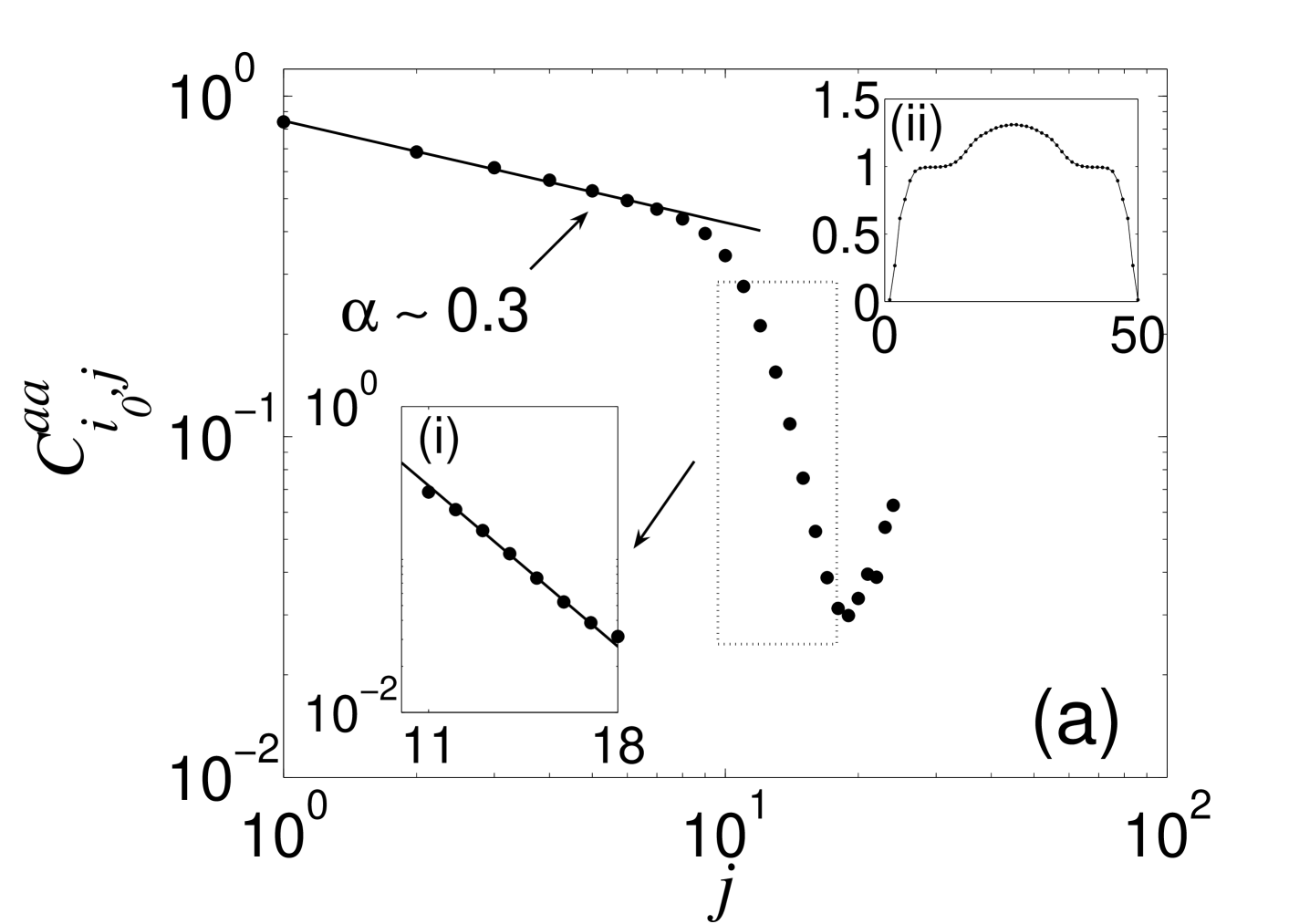
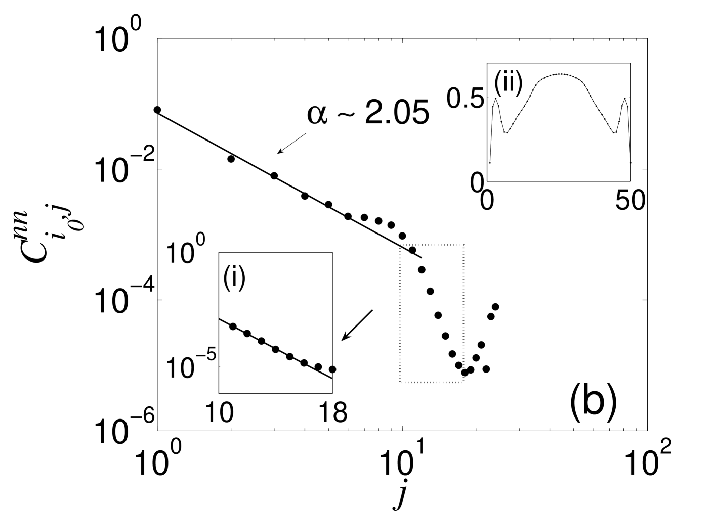
Figure 7: Correlation functions (a) $C^{aa}_{i_{0},j}$ and (b) $C^{nn}_{i_{0},j}$ in a linear Paul trap when $U/t=2$ ($N=N_{\textmd{ph}}=50$). Both of them show the coexistence of superfluid and Mott-insulator phases. In (a) and (b), the insets (i) show the exponential decay in the region of the Mott phase, and the insets (ii) show the occupation number and fluctuations at the same parameters. The exponents $\alpha$ of the algebraic decay are also given in the figures. The dotted and solid lines are numerical and fitting data, respectively.

IV.2 Mott-insulator phase

In the commensurate case, by increasing the on-site interaction $U$, a quantum phase transition from a superfluid to a Mott-insulator state takes place at about $U\approx 2t$. In the limit in which interaction dominates over hopping, the ground state for a commensurate filling of $\bar{n}$ particles per site is simply a product state of local phonon Fock states,

$$|\psi_{MI}\rangle=\prod_{i=1}^{N}\frac{1}{\sqrt{\bar{n}!}}(a^{\dagger}_{i})^{\bar{n}}|0\rangle.$$ (21)

In the Mott insulator phase correlations decay exponentially with distance, $C^{aa,nn}_{i,j}\propto{\textrm{e}}^{-|i-j|/\xi}$, where $\xi$ is the correlation length. The correlation length diverges when approaching the quantum phase transition.

(1) Array of ion microtraps. In Fig. 8 (a) we plot the correlation functions in the phonon Mott phase in the case of an array of ion microtraps. These curves can be fitted to an exponential decay, and the correspond correlation lengths are plotted in Fig. 8 (b) as a function of the interaction strength. Due to the finite size of the system, $\xi$ does not diverge at the critical value of $U$. However, the extrapolation of the curves in the linear regime allows us to estimate the critical point, which lies at $U_{c}/t\approx 1.55$. This critical value is smaller than the one in the BHM with tunneling between nearest–neighbors only, $U^{nn}_{c}/t\approx 2$. The condition $U_{c}<U_{c}^{nn}$ is due to the frustration induced by hopping between next–nearest–neighbors, which makes the superfluid phase more unstable against the effect of on–site interactions.

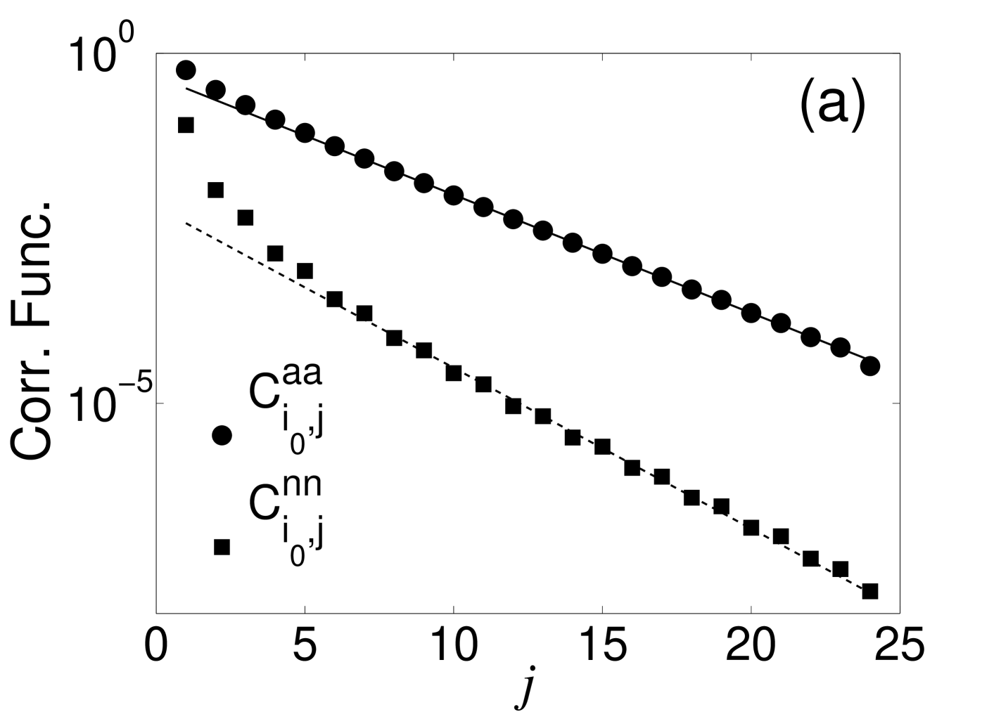
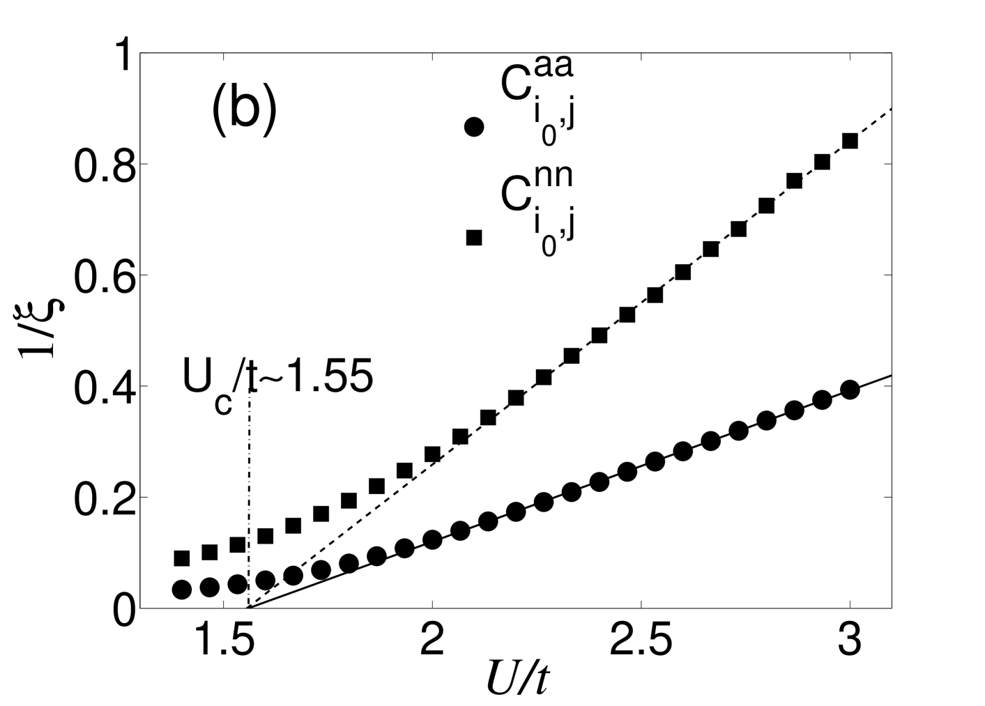
Figure 8: (a) Correlation functions $C^{aa}_{i_{0},j}$ at $U/t=3$ and $C^{nn}_{i_{0},j}$ at $U/t=2.4$ decay exponentially with the coordinate $j$ at the Mott-insulator phase for an array of microtraps ($N=N_{\textmd{ph}}=50$, $i_{0}=26$). (b) The inverse of the correlation lengths in $C^{aa}_{i_{0},j}$ and $C^{nn}_{i_{0},j}$. The circle markers represent $C^{aa}_{i_{0},j}$ and the square markers $C^{nn}_{i_{0},j}$. The solid lines are the fitting data. The extrapolation in (b) show that the critical point in the microtraps is $U_{c}/t\approx 1.55$.

(2) Linear ion trap. In the case of a linear trap, the behavior of spatial correlations is similar, see Fig. 9. $C^{nn}_{i,j}$ is difficult to fit due to the few points with exponential decay, therefore we only plot the correlation length corresponding to $C^{bb}_{i,j}$.

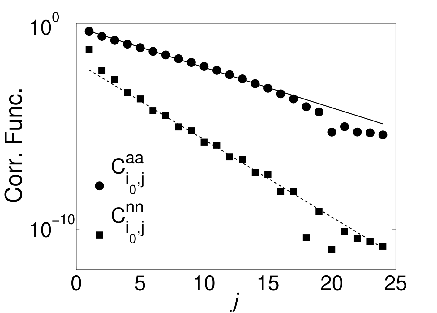
Figure 9: The exponential decay correlations $C^{aa}_{i_{0},j}$ and $C^{nn}_{i_{0},j}$ at the Mott phase $U/t=2.8$ for a linear Paul trap ($N=N_{\textmd{ph}}=50$, $i_{0}=26$).

Due to the effective phonon trapping potential, the Mott insulator and superfluid phases coexist in a range of values of $U$ (Fig. 7). For this reason, in the case of a linear Paul trap, one cannot follow the extrapolation procedure of Fig. 8 to find a critical value of the interaction.

Finally, in the Mott-insulator phase the long-range hopping terms which decay like $1/|z^{0}_{i}-z^{0}_{j}|^{3}$ play a major role, since they induce a peculiar long-range correlation in this phase. In Fig. 10, we show that $C^{aa}_{i,j}$ indeed also behaves like $1/|z^{0}_{i}-z^{0}_{j}|^{3}$ at long distances. The existence of power–law decay in correlation functions of non–critical systems due to long–range interactions was also observed in the case of spin models in trapped ions, see the discussion in Ref. DengPorrasCirac.spin .

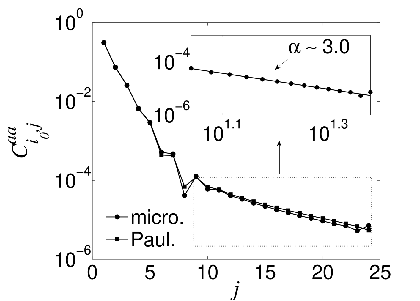
Figure 10: The correlation $C^{aa}_{i_{0},j}$ at the Mott phase $U/t=6$ in an array of microtraps (circle markers) and a linear Paul trap (square markers), respectively. $N=N_{\textmd{ph}}=50$, $i_{0}=26$. The inset shows the power-law decay with exponent $\alpha\approx 3$ for the microtraps only.

IV.3 Tonks-gas phase

We turn now to the incommensurate filling case, where in the limit $U\gg t$ the system forms a Tonks-Girardeau gas, which can be described in terms of effective free fermions. A Tonks-Girardeau gas has recently been realized in an experiment with ultracold bosons in an optical lattice Paredes.Tonks .

(1) Array of ion microtraps. We have studied numerically the Tonks–Girardeau regime in the case of phonons in ion traps, starting with the case of an array of ion microtraps with $N=50$ sites and $N_{ph}=25$ phonons, that is, $1/2$ filling. The density of phonons evolves from a superfluid to a Tonks-gas profile when increasing the interaction, and at the end it approaches a constant value of $1/2$. Correlation functions decay algebraically, with an exponent that approaches $\alpha\approx 0.58$ for large interactions (see Fig. 11). Note that $\alpha$ deviates from $1/2$, which is the value that corresponds to a Tonks gas with nearest–neighbor tunneling only. The deviation can be explained by the mapping from the BHM model (14) with $U\gg t$ to an XY model with antiferromagnetic interactions of the form $J_{i,j}=J/|i-j|^{3}$. The long–range terms in the antiferromagnetic interaction induces a change in the exponent of the correlation functions, as shown with the numerical calculations of our previous work on spin models in ion traps DengPorrasCirac.spin .

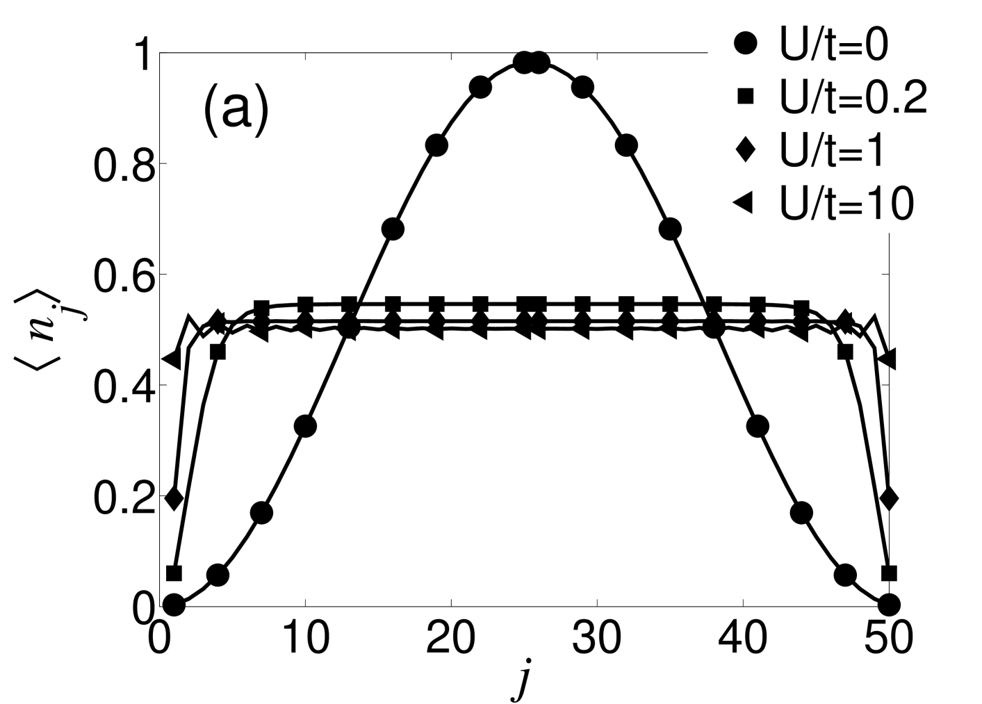
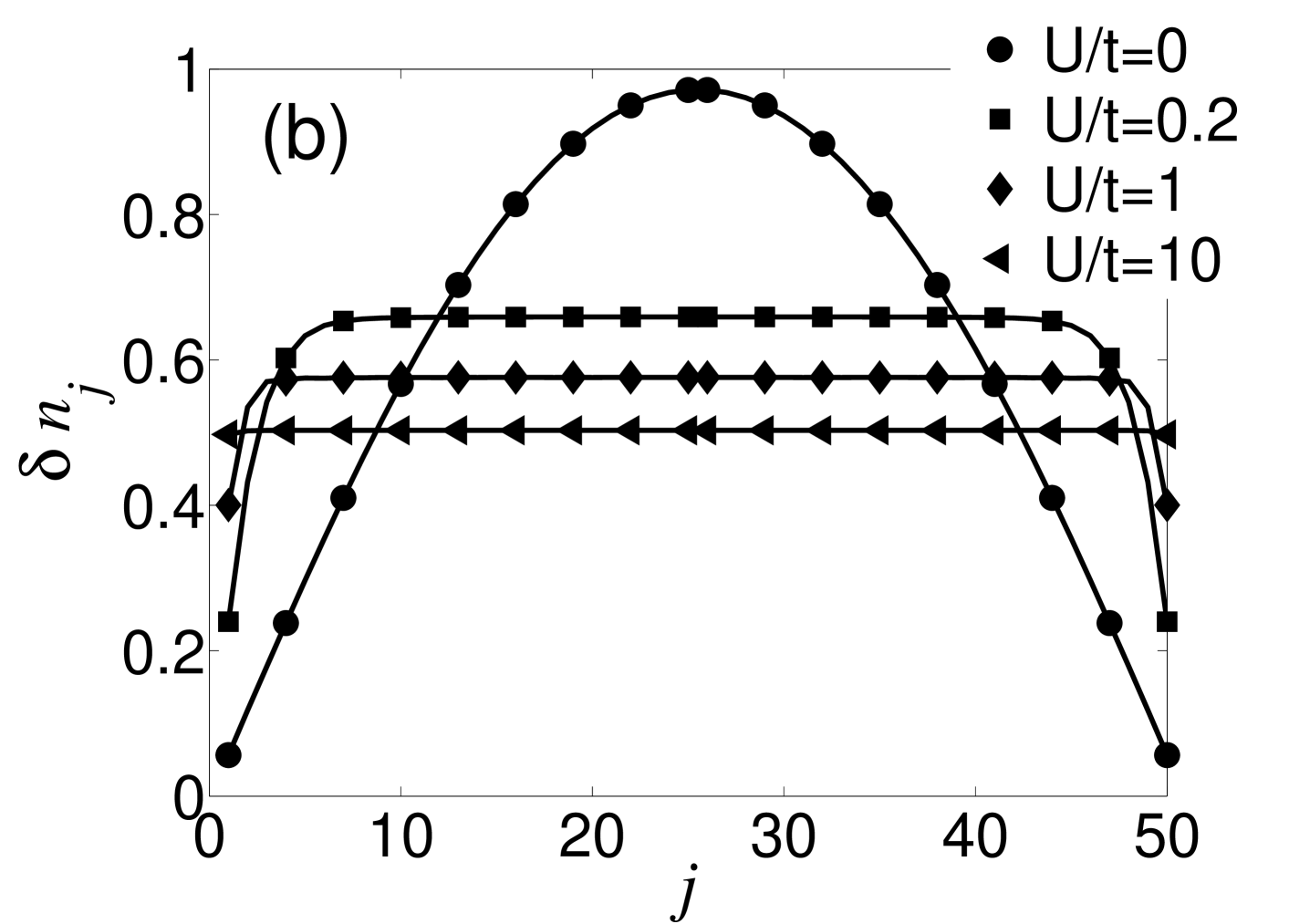
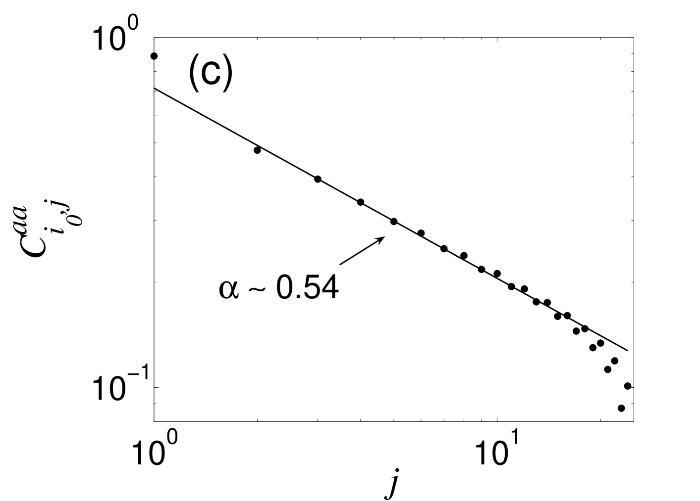
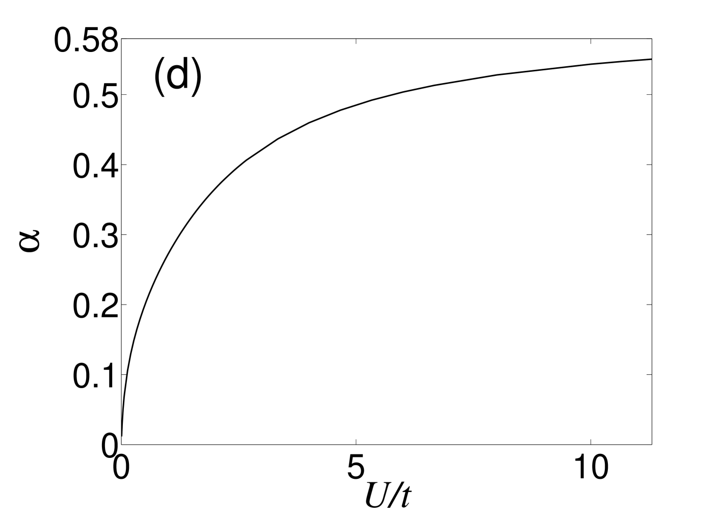
Figure 11: (a) Densities of phonons in an array of microtraps with $N=50$, $N_{ph}=25$. (b) Fluctuations at the same conditions. (c) The correlation function $C^{aa}_{i_{0},j}$ ($i_{0}=26$) at Tonks-gas phase $U/t=10$ with exponent $\alpha\approx 0.54$, where the dotted and solid lines are numerical and fitting data, respectively. (d) Evolution of exponent $\alpha$ of $C^{aa}_{i_{0},j}$ with the interaction $U/t$, which would approach $\alpha\approx 0.58$.

(2) Linear ion trap. We study now the case of phonons in a linear Paul trap under the same conditions, see Fig. 12. Correlation functions decay algebraically, with an exponent that is extrapolated to $\alpha=0.53$ in the limit of strong interactions. This result can also be explained by the mapping to the $XY$ model, and coincides with the result found in DengPorrasCirac.spin .

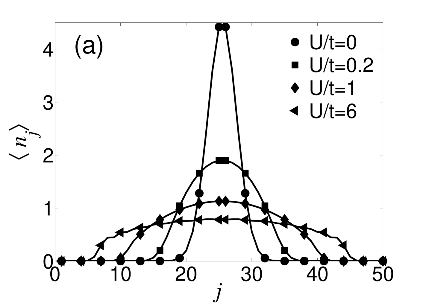
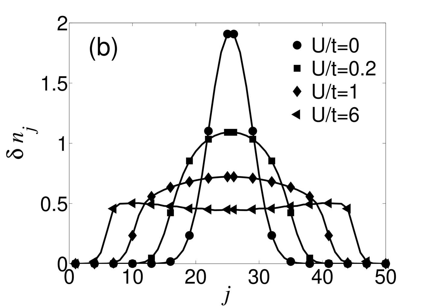
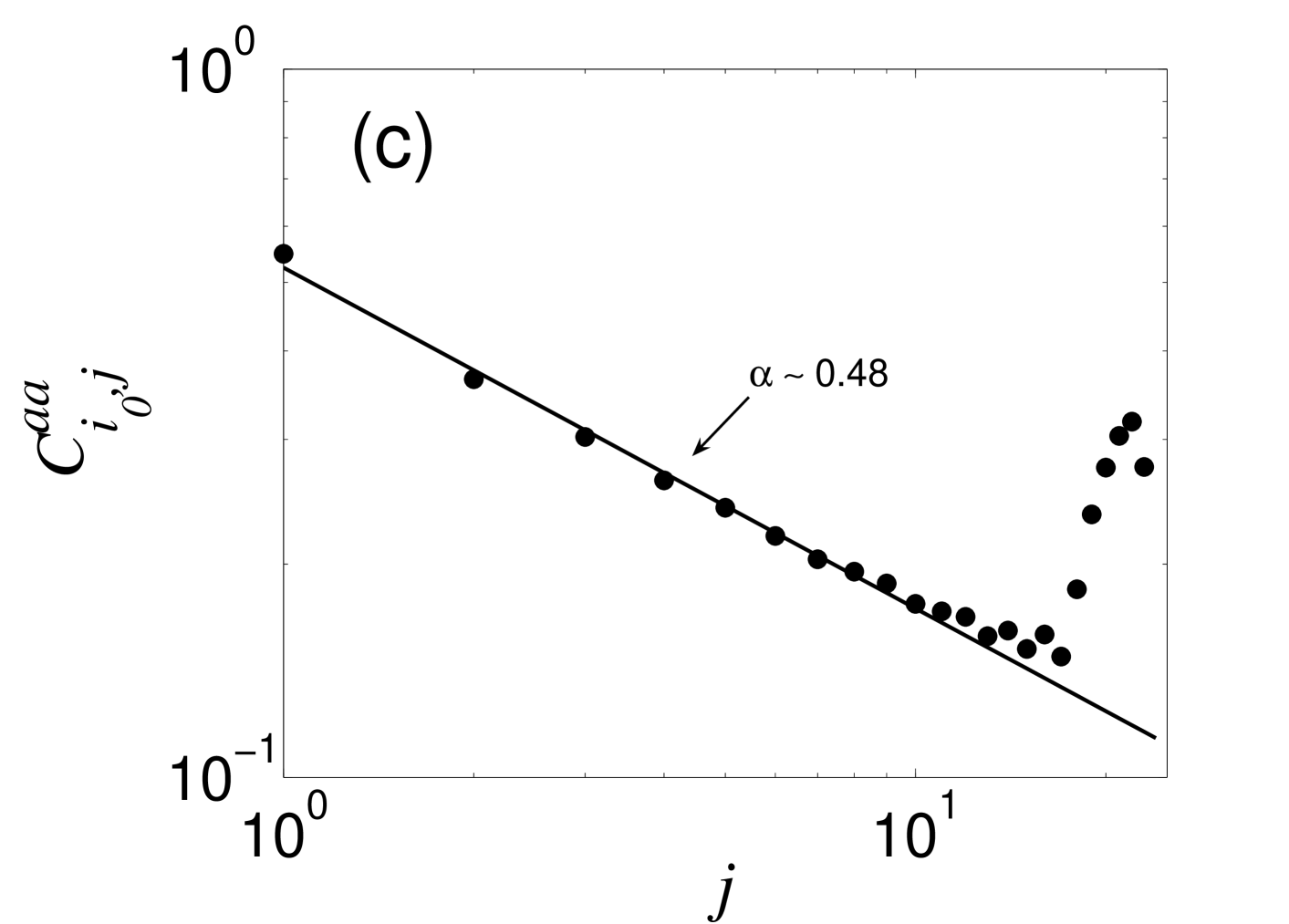
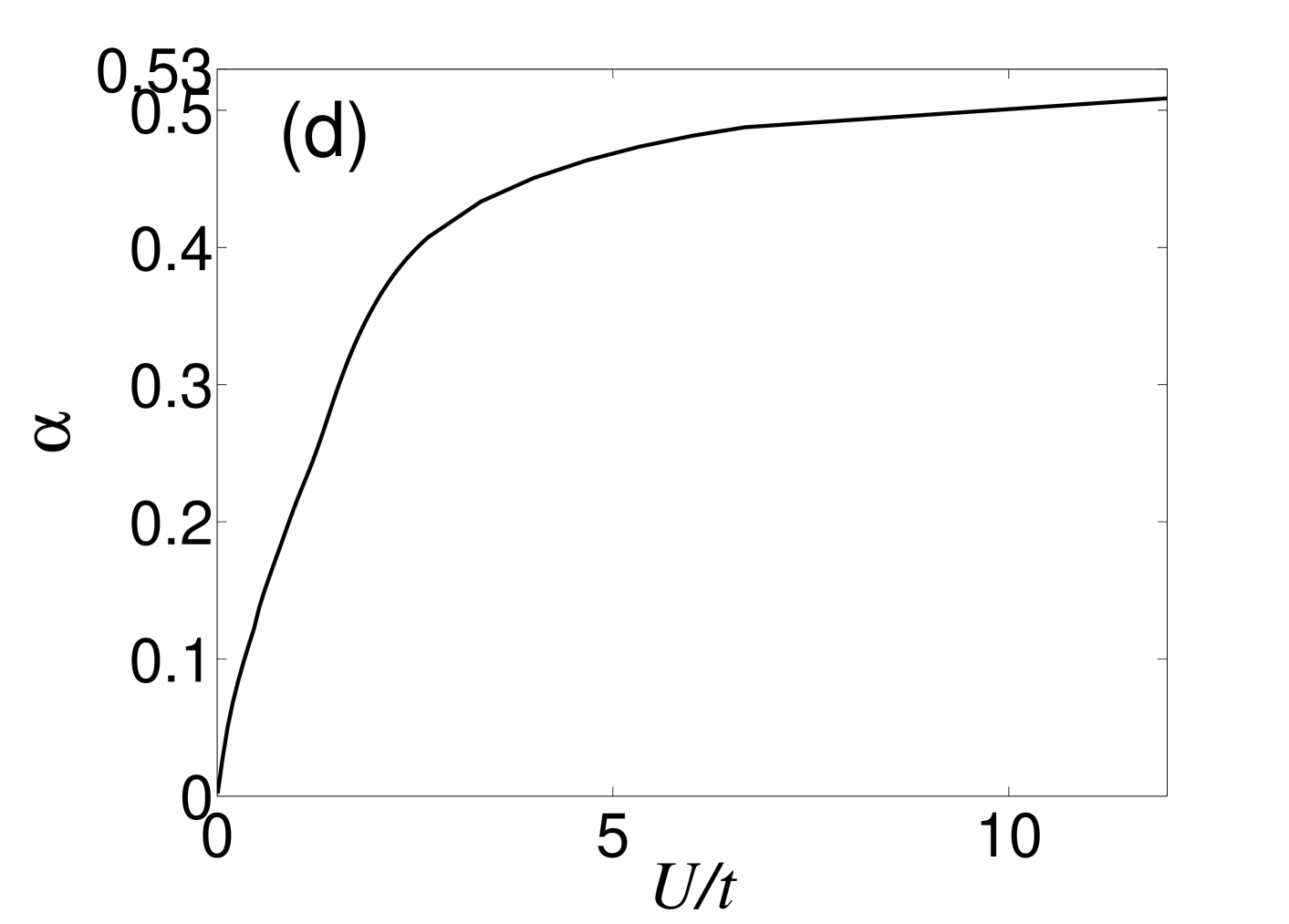
Figure 12: (a) and (b) show densities and fluctuations of phonons, respectively, in a linear Paul trap with $N=50$ and $N_{ph}=50$; (c) The correlation $C^{aa}_{i_{0},j}$ at the Tonks-gas phase $U/t=6$, whose exponent is $\alpha\approx 0.48$; (d) Evolution of the exponents $\alpha$ of $C^{aa}_{i_{0},j}$, approaching $\alpha\approx 0.53$. In (c) the dotted and solid lines represent numerical and fitting data, respectively.

In order to test if the system is really in the Tonks–gas phase, we introduce the quantity $\langle O\rangle=\langle\sum_{i}n_{i}(n_{i}-1)\rangle/N$, which measures the probability of phonon occupancies larger than one. In the Tonks–gas regime $\langle O\rangle\sim 0$. The parameter $\langle O\rangle$ as a function of the interaction $U$ is plotted in Fig. 13, showing the continuous evolution into the Tonks–gas regime.

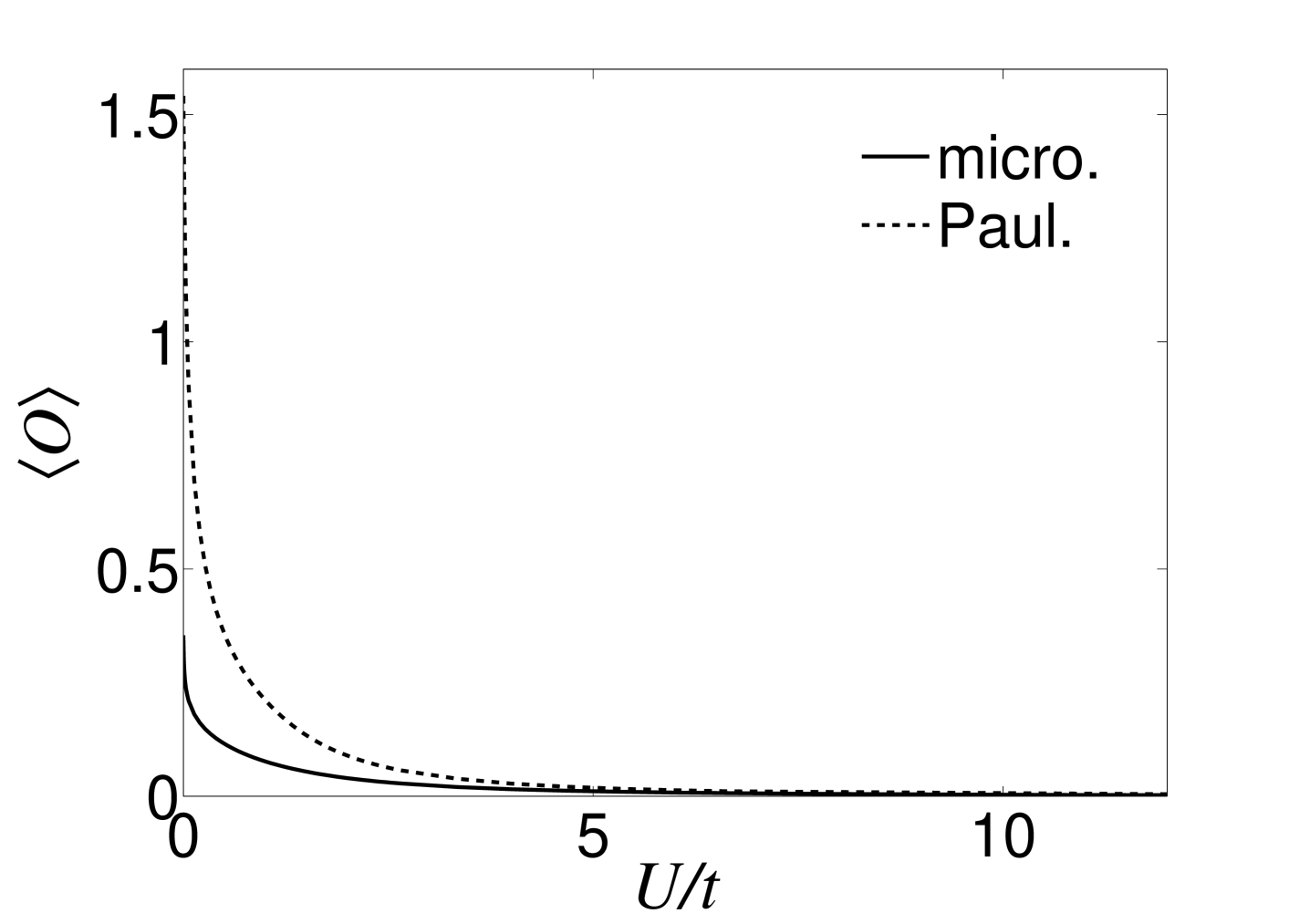
Figure 13: The evolution of the parameter $\langle O\rangle$ with the interaction $U/t$ in an array of microtraps (solid line) and a linear Paul trap (dashed line). $N=50$, $N_{\textmd{ph}}=25$.

Our results are consistent with the behaviors observed in optical lattices Paredes.Tonks . The numerical analysis shows that phonons in ion traps are also a good candidate like atoms in optical lattices for studying Tonks gases.

V Bose-Hubbard model with Attractive interactions: $U<0$

The BHM with attractive interactions in optical lattices has been the focus of recent theoretical studies JackYamashita . The sign of phonon–phonon interactions in trapped ions can be made negative simply by changing the relative position of the standing–wave relative to the ion chain. For a qualitative understanding of this model, it is useful to consider a Bose–Einstein condensate in a double well potential JackYamashita ; SteelCollett . In a symmetric potential in the absence of tunneling, energy is decreased when bosons accumulate in one of the wells. When tunneling is switched on, the ground state of the system is a linear superposition of states with all the bosons placed in one of the wells, showing large phonon number fluctuations.

The increase of phonon number fluctuations in our model when we switch on a negative interaction is also shown in our numerical calculations. In Fig. 14, the density at the center of the ion chain and its fluctuations increase with the magnitude of the interaction for $N=10$ ions and $N_{ph}=10$ phonons with open boundary conditions. Due to the open boundary condition and the symmetry of the potential, the phonons tend to collect themselves on one of the two sites at the center when increasing $|U|$ with an even number of sites. The ground state is then a superposition of $N_{ph}$ phonons on site $N/2$ and $N_{ph}$ phonons on site $N/2+1$.

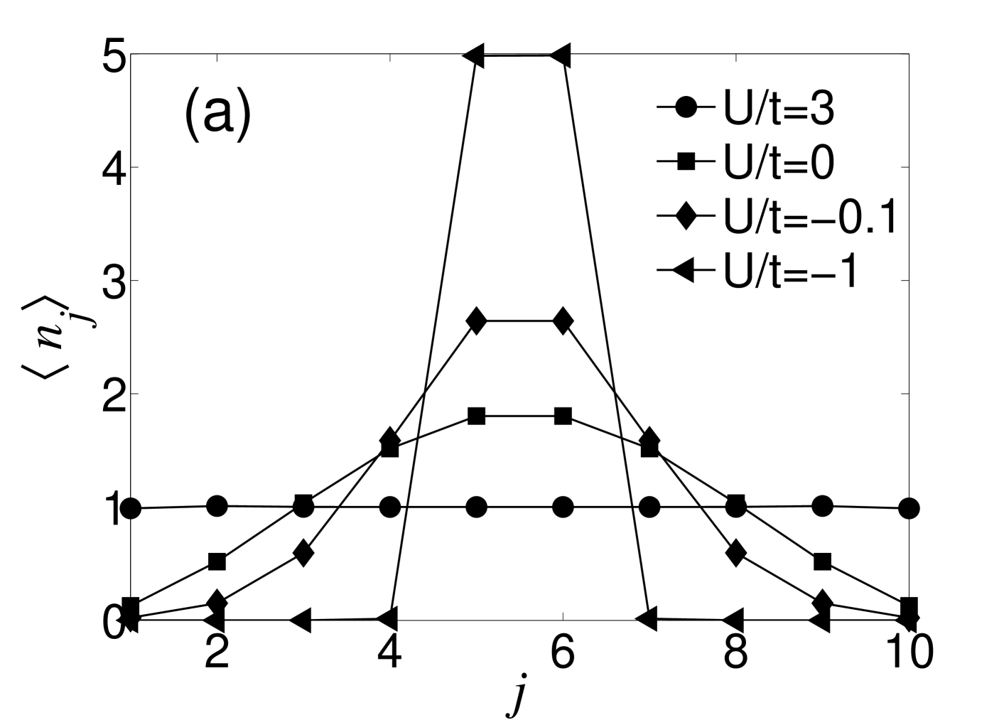
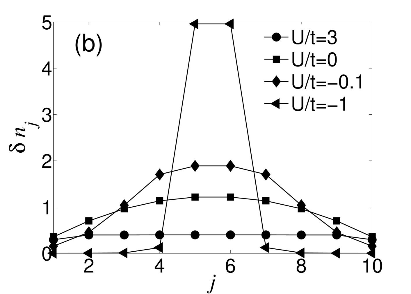
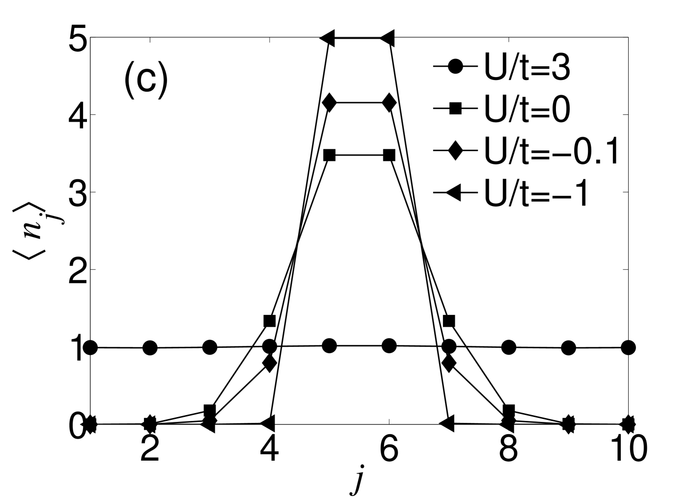
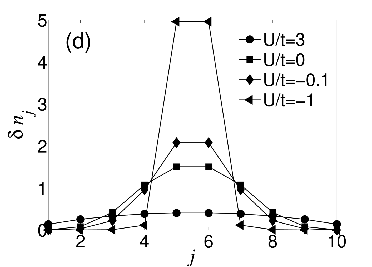
Figure 14: (a) Density of phonons and (b) phonon number fluctuations in an array of microtraps with $N=10$, $N_{ph}=10$, and negative on–site interactions . (c) Density of phonons and (d) phonon number fluctuations in a linear Paul trap under the same conditions.

When $|U|$ is large enough, our numerical calculations yield a ground state with all the phonons in a single ion, such that the spatial symmetry of the problem is broken. This effect is an artifact of the DMRG calculation, due to the small energy difference between the exact ground state of the system and the one which breaks the spatial symmetry. Thus, in order to study properly the phonon phases with negative interaction, it is convenient to define the following order parameter, whose value is independent on the breaking of the spatial symmetry in the problem:

$$\langle O\rangle=\frac{1}{N^{2}}\langle\sum_{j}(a^{\dagger}_{j}a_{j})^{2}\rangle.$$ (22)

In Fig. 15 we show the evolution of this quantity, which shows a sudden increase for negative interactions.

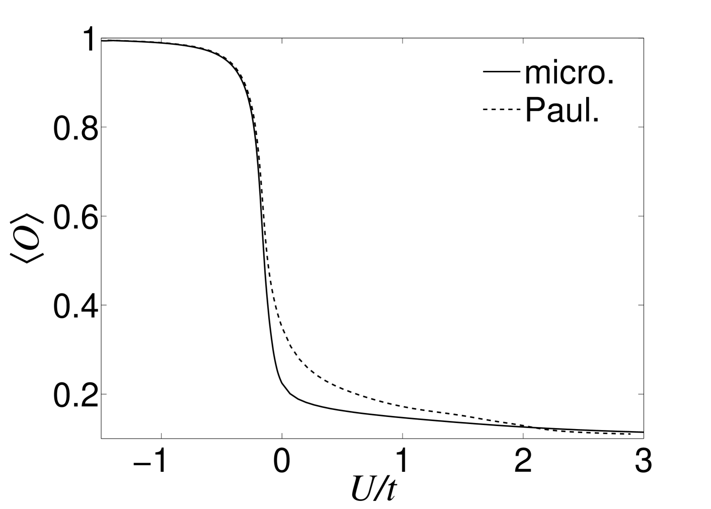
Figure 15: Evolution of the order parameter $\langle O\rangle$ with the ratio $U/t$ for an array of ion microtraps (solid line) and a linear Paul trap (dashed line). $N=N_{\textmd{ph}}=10$.

VI Bose-Hubbard model with site-dependent interactions

Phonons in trapped ions have a higher controllability than ultracold neutral atoms in optical lattices, due to the possibility of individual addressing. In particular, on–site interactions can be induced in such a way that they depend on the ion position. In this section we present a model which shows how this possibility can be exploited for the engineering of quantum phases.

Let us consider repulsive on-site interactions which vary over the ion chain in the following way:

$$U_{i}=U_{\textmd{odd}}=U,\hskip 17.07182pt \textmd{i odd},$$

$$U_{i}=U_{\textmd{even}}=2U,\hskip 17.07182pt \textmd{i even},$$ (23)

We focus on the case with filling factor 2, $N_{\textmd{ph}}=2N$, in the regime where interactions dominate over tunneling, $U/t\gg 1$. In the limit $t=0$, the ground state of this model is highly degenerate. For instance, in a chain with two sites the ground state manifold in the Fock basis spans the states $|2,2\rangle$ and $|3,1\rangle$. In a chain with even number $N$ of sites and $N_{\textmd{ph}}=2N$, the ground state degeneracy is $\left(\begin{array}[]{c}N\\ N/2\end{array}\right)$ .

Our DMRG algorithm allows us to calculate the density and fluctuations in the phonon number, which are shown in Fig. 16, for the case where the interactions defined by Eq. (23) are induced on an array of ion microtraps. In the ground state of the chain, the number of phonons fluctuates between $|2\rangle$ and $|3\rangle$, and $|2\rangle$ and $|1\rangle$, in odd and even sites, respectively.

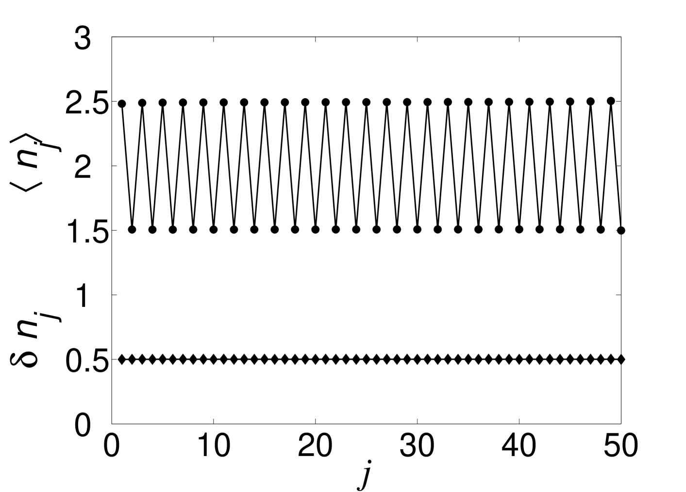
Figure 16: The phonon density $\langle n_{j}\rangle$ and phonon number fluctuations, $\delta n_{j}$, in an array of ion microtraps, with the on–site interactions defined by Eq. (23), $U/t=40$, $N=50$, and $N_{ph}=2N=100$.

This model can be understood in the hard–core boson limit by introducing a spin representation, which is valid near filling factor 2. At each site in the ion chain, we define a two level system by means of the following rule:

$$|\bar{0}\rangle_{i}=|2\rangle_{i},\hskip 5.69046pt|\bar{1}\rangle_{i}=|3\rangle_{i},\hskip 2.84544pt \textmd{i odd},$$

$$|\bar{0}\rangle_{i}=|1\rangle_{i},\hskip 5.69046pt|\bar{1}\rangle_{i}=|2\rangle_{i},\hskip 2.84544pt \textmd{i even}.$$ (24)

Where $|\bar{0}\rangle$ and $|\bar{1}\rangle$ are the two levels which define the spin states of the spin representation of the hard–core bosons. Spin and phonon annihilation operators satisfy:

$$\sigma^{+}_{i} = \frac{1}{\sqrt{3}}a^{\dagger}_{i},\hskip 5.69046pt\textmd{i odd},$$

$$\sigma^{+}_{i} = \frac{1}{\sqrt{2}}a^{\dagger}_{i},\hskip 5.69046pt\textmd{i even}.$$ (25)

where the equality is understood to hold within the ground state manifold. In terms of this operators, the Hamiltonian of the system is described by an XY model (for simplicity we consider here the nearest-neighbor case):

$$H={\tilde{J}}\sum_{i}(\sigma^{+}_{i}\sigma^{-}_{i+1}+h.c.),$$ (26)

with ${\tilde{J}}=\sqrt{6}t$. Under the condition $N_{\textmd{ph}}/N=2$, the ground state of our hard–core boson Hamiltonian corresponds to the solution of the $XY$ model (26) with the constraint $\sum_{i}\sigma^{z}_{i}=0$.

Spin-spin correlation functions are related to the bosonic correlations functions of the BHM by the relation Eq. (25). In Fig. 17 we plot $\langle\sigma^{+}_{i}\sigma_{j}\rangle$ calculated by means of correlation functions of hard–bosons. This correlation function shows an algebraic decay for short distances, which is spoiled for long separations between ions due to boundary effects. The exponent $\alpha\sim 0.56$, differs from the one that we expect from the mapping to the XY model, that is, $\alpha=0.5$, due to the effect of further than nearest–neighbor interactions terms, which we have neglected.

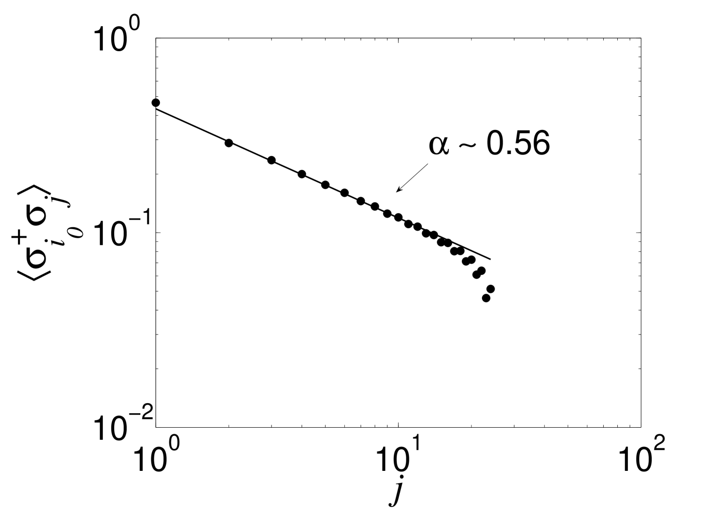
Figure 17: The correlation function $\langle\sigma^{+}_{i_{0}}\sigma_{j}\rangle$ defined by (24). $i_{0}=26$, $N=50$, $N_{\textmd{ph}}=100$, $U/t=40$.

Another interesting possibility is to study the phase diagram of the BHM with filling factor 2, and alternating interactions, beyond the $XY$ point $U_{\textmd{even}}=2U_{\textmd{odd}}$. If we change the ratio $U_{\textmd{even}}/U_{\textmd{odd}}$ in the vicinity of this point, the ground state degeneracy with zero tunneling is lifted. The system is in a Mott insulator phase, with constant phonon density if $U_{\textmd{even}}>2U_{\textmd{odd}}$, $|2,2,2,\dots\rangle$, or alternating occupation numbers if $U_{\textmd{even}}<2U_{\textmd{odd}}$ , $|3,1,3,1,\dots\rangle$. The phase diagram as a function of the ratio $U_{\textmd{even}}/U_{\textmd{odd}}$, shows two gaped regions, separated by a single critical point, which corresponds to the $XY$ limit studied above. This is shown in Fig. 18, where we calculate the energy gap $\Delta E$ for small chains ($N=6$).

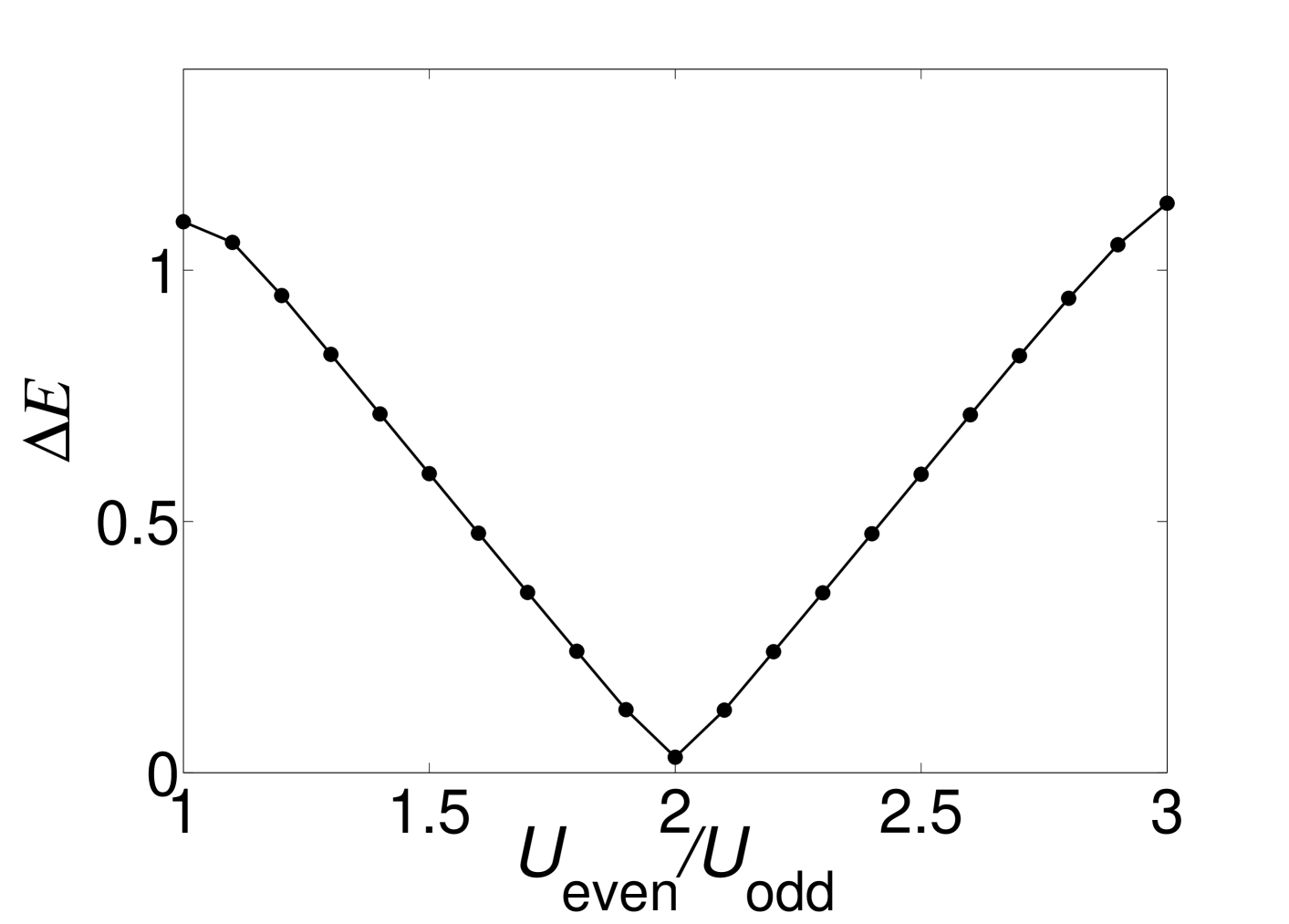
Figure 18: The energy gap $\Delta E$ between the ground state and the first excited state as a function of $U_{\textmd{even}}/U_{\textmd{odd}}$. $U_{\textmd{odd}}/t=40$. For simplicity, we consider here a small system of ions $N=6$.

To generalize, the same also takes place with other distributions of the on–site interactions, whenever the number of sites where phonons interact with $U$ is the same as the number of sites with $2U$ interaction. For example, the chain can be divided in two regions, left and right, such that the interactions depend on the site in the way $U,U,...,2U,2U,...$, that is, $U_{i}=U_{\textmd{left}}=U$ and $U_{i}=U_{\textmd{right}}=2U$.

VII Conclusions

In conclusion, we have studied the quantum phases of interacting phonons in ion traps. The superfluid–Mott insulator quantum phase transition can be detected by the evolution of the phonon density profile, as well as by the divergence of the correlation length near the quantum critical point. Although boundary effects are important, specially in the case of a Coulomb chain of ions, correlation functions show a similar behavior as those of systems in the thermodynamical limit. For example, Luttinger liquid theory gives an approximate description of the algebraic decay of correlations in the superfluid regime.

We have also shown that the ability to control phonon–phonon interactions allows us to study a variety of situations like attractive interactions, where a phase with large phonon number fluctuations takes place. The ability to tune locally the value of the on–site interactions also leads to the realization of new exciting models, where the degeneracy of the classical ground state can be tuned by choosing properly the value of the phonon–phonon interactions.

Work supported by the Deutscher Akademischer Austausch Dienst, SCALA and CONQUEST projects and the DFG.

References

- (1)
- (2)
- (3) D. Jaksch, C. Bruder, J.I. Cirac, C. Gardiner and P. Zoller, Phys. Rev. Lett. 81, 3108 (1998); M. Greiner, T. Esslinger, T.W. Haensch and I.Bloch, Nature 415, 39 (2001).
- (4) D. Porras and J.I. Cirac, Phys. Rev. Lett. 92, 207901 (2004).
- (5) D. Porras and J.I. Cirac, Phys. Rev. Lett. 93, 263602 (2004).
- (6) X.-L. Deng, D. Porras, and J.I. Cirac, Phys. Rev. A 72, 063407 (2005).
- (7) J. P. Barjaktarevic, G. J. Milburn, and Ross H. McKenzie Phys. Rev. A 71, 012335 (2005).
- (8) D. Porras and J.I. Cirac, Phys. Rev. Lett. 96, 250501 (2006).
- (9) D. Leibfried, R. Blatt, C. Monroe, and D. Wineland, Rev. Mod. Phys. 75, 281 (2003).
- (10) D.M. Meekhof, C. Monroe, B.E. King, W.M. Itano, and D.J. Wineland, Phys. Rev. Lett. 76, 1796 (1996).
- (11) M. Fisher, P. Weichman, G. Grinstein, and D. Fisher, Phys. Rev. B 40, 546 (1989).
- (12) S. Sachdev, Quantum Phase transitions (Cambridge University Press, Cambridge, U.K. 1999).
- (13) S. White, Phys. Rev. Lett. 69, 2863 (1992); S. White, Phys. Rev. B. 48, 10345 (1993).
- (14) U. Schollwöck, Rev. Mod. Phys. 77, 259 (2005).
- (15) C. Kollath, U. Schollwöck, J. von Delft, and W. Zwerger, Phys. Rev. A 69, 031601(R) (2004).
- (16) F.M.D. Haldane, Phys. Rev. Lett. 47, 1840 (1981).
- (17) D.M. Gangardt and G.V. Shlyapnikov, Phys. Rev. Lett. 90, 010401 (2003).
- (18) K.V. Kheruntsyan, D.M. Gangardt, P.D. Drummond, and G.V. Shlyapnikov, Phys. Rev. A 71, 053615 (2005).
- (19) Note that long–range order is destroyed by quantum fluctuations even at zero temperature in one spatial dimension. However we use here the usual terminology in lattice models, and choose the term “superfluid phase” for the quantum phase of the Bose–Hubbard model. This phase does not show long–range order, but algebraic decay of the phase correlations.
- (20) B. Paredes, A. Widera, V. Murg, O Mandel, S. Fölling, I. Cirac, G. V. Shlyapnikov, T. W. Hänsch and I. Bloch, Nature 429, 227 (2004).
- (21) M.W. Jack and M. Yamashita, Phys. Rev. A. 71, 023610 (2005).
- (22) M.J. Steel and M.J. Collett, Phys. Rev. A 57, 2920 (1998).