Transport and Entanglement Generation in the Bose-Hubbard Model

Abstract

We study entanglement generation via particle transport across a one-dimensional system described by the Bose-Hubbard Hamiltonian. We analyze how the competition between interactions and tunneling affects transport properties and the creation of entanglement in the occupation number basis. Alternatively, we propose to use spatially delocalized quantum bits, where a quantum bit is defined by the presence of a particle either in a site or in the adjacent one. Our results can serve as a guidance for future experiments to characterize entanglement of ultracold gases in one-dimensional optical lattices.

, , , and

1 Introduction

The generation of entanglement between distant nodes of a quantum network has profound implications for quantum computation and information [1], and has triggered a remarkable effort into the study of entanglement generation and quantum state transport between distant lattice sites (see, e.g., Refs. [2, 3, 4, 5] for discussions of transport in spin chains; entanglement dynamics in such systems is, e.g., studied in [6, 7, 8]). Furthermore, the recent experimental achievements in loading either bosonic and/or fermionic ultracold atomic gases into optical lattices, which permits to reproduce very accurately several spin Hamiltonians, have spurred an enormous interest in lattice systems (see [9] and references therein).

Here we focus on one of the simplest but yet non-trivial lattice model, the so-called one-dimensional (1D) Bose-Hubbard Model (BHM) [10, 11]. It describes a system of spinless bosons with (repulsive) on-site interaction, which can hop (tunnel) between adjacent sites of a 1D lattice. In general, this genuinely many-body model cannot be reduced to an effective non-interacting one. As proposed in [12] and later experimentally demonstrated [13], it can be realized by confining ultracold atoms in an optical lattice. In this article we study transport properties in this system. Here, by transport we refer to the dynamics obtained when an extra particle is loaded onto a system that previously was cooled to its ground state. In some limiting cases, transport can be described in the language of continuous time quantum walks (a quantum analogue of classical random walks) and closed analytical expressions can be found [14]. When competition between hoping and on-site interactions arises, the transport properties as well as the generation of entanglement between distant locations of the lattice is substantially modified.

The article is structured as follows: in the present section we review the essential properties of the Bose-Hubbard model. As one limiting case we identify transport across the lattice with continuous time quantum walks. We discuss quantification and characterization of entanglement for a single particle propagating in a 1D lattice. In Sec. 2, we analyze the generation of entanglement between distant lattice sites when an extra particle is loaded on top of the ground state. In Sec. 3, we discuss entanglement in the so-called Spatially Delocalized Qubit (SDQ) basis and investigate the role of interactions within this scheme. Finally, we summarize briefly in Sec. 4.

1.1 The Bose-Hubbard Hamiltonian

The Bose-Hubbard Hamiltonian for a 1D lattice of $M$ sites (with open-boundary conditions) has the form

$$\hat{H}_{\rm BH}=-J\sum_{i=1}^{M-1}\left(\hat{a}^{{\dagger}}_{i}\hat{a}_{i+1}+\hat{a}^{{\dagger}}_{i+1}\hat{a}_{i}\right)+\sum_{i=1}^{M}\epsilon_{i}\hat{n}_{i}+\frac{U}{2}\sum_{i=1}^{M}\hat{n}_{i}(\hat{n}_{i}-1),$$ (1)

where $\hat{a}_{i}$ and $\hat{a}^{{\dagger}}_{i}$ are the bosonic annihilation and creation operators for a particle on the $i$-th lattice site, $\hat{n}_{i}=\hat{a}^{{\dagger}}_{i}\hat{a}_{i}$ is the corresponding bosonic number operator, and $\epsilon_{i}$ accounts for the single-particle on-site energy. The Bose-Hubbard model assumes only nearest-neighbour tunneling with constant amplitude $J$ and pairwise interaction between bosons on the same site leading to an energy shift $U$.

A particularly clean realization of such a Hamiltonian is obtained by trapping neutral bosons via the dipole force in an optical lattice [12]. By taking the trapping sufficiently tight in two directions (say $y$ and $z$), an effective one-dimensional system can be realized. The corresponding Hamiltonian in second quantization notation reads

$$\hat{\mathcal{H}}_{\rm OL} = \int dx\,\hat{\psi}^{\dagger}(x)\left(\frac{p_{x}^{2}}{2m}+V_{0}\sin^{2}(\pi x/d)\right)\hat{\psi}(x)+g\int dx\,\hat{\psi}^{\dagger}(x)\hat{\psi}^{\dagger}(x)\hat{\psi}(x)\hat{\psi}(x)$$ (2)

$$\equiv \int dx\,\hat{\psi}^{\dagger}(x)H_{\rm free}\hat{\psi}(x)+\hat{\mathcal{H}}_{\rm int}.$$

The optical lattice is completely characterized by its depth $V_{0}$, that can be controlled through the laser intensity, and by the wave number ${\it k}=2\pi/\lambda$ where $d=\lambda/2$ is the lattice periodicity. The effective 1D interaction strength $g=2\pi\hbar a_{s}\omega_{t}$ (where $\omega_{t}$ is the transversal frequency of the trap assumed equal in the $y,z$ directions and $a_{s}$ is the atomic scattering length) can be changed either by modifying the confinement of the atoms in the two orthogonal directions or, alternatively, via a Feshbach resonance, which even allows to change the sign of $a_{s}$ [15]. For periodic boundary conditions (or large enough lattices) the bosonic operators can be expanded in terms of Bloch functions. In the low temperature regime and with typical bosonic interaction strengths, excitations to higher bands can be neglected for sufficiently deep lattices. The dynamics is then restricted to the lowest Bloch band and the field operators can be expanded in terms of single-particle Wannier functions localized at each lattice site $x_{i}=d\,i$ as $w(x-x_{i})\equiv\langle x|w_{i}\rangle$. The bosonic creation operators $\hat{a}^{{\dagger}}_{i}$ are now defined via $|w_{i}\rangle=\hat{a}^{{\dagger}}_{i}|\Omega\rangle$, $|\Omega\rangle$ being the vacuum. Eq. (1) is derived from Eq. (2) by keeping only nearest-neighbor hopping and restricting the interactions between bosons to a contact (zero-range) potential. Under these approximations, the tunneling amplitude between adjacent sites reads $J=\langle w_{i}|H_{\rm free}|w_{i+1}\rangle$, and the on-site boson-boson interaction is given by $U=g\int dx|w(x)|^{4}$.

The Bose-Hubbard ground state with filling factor $\bar{n}$ is obtained by minimizing $\langle\hat{H}_{\rm BH}-\mu\sum_{i}\hat{n}_{i}\rangle$, where the chemical potential $\mu$ fixes the total number of particles. In the limit $U/J\rightarrow 0$ (strictly speaking, in the thermodynamic limit for $U/J<(U/J)_{c}\approx 3.44$ for $\bar{n}=1$ [16]) it is energetically favorable to spread each particle over the whole lattice. For periodic boundary conditions, a ground state with filling factor $\bar{n}$ can be explicitly written as

$$|\psi^{\bar{n}}_{\rm GS,SF}\rangle=\frac{1}{\sqrt{(M\bar{n})!}}\left(\frac{1}{\sqrt{M}}\sum_{i}^{M}\hat{a}^{{\dagger}}_{i}\right)^{{M\bar{n}}}|\Omega\rangle,$$ (3)

where $M\bar{n}$ is the total number of particles. This superfluid (SF) state is characterized by large fluctuations of the on-site number of particles, divergent correlation length, and a vanishing gap. In the opposite limit, for $U/J\rightarrow\infty$, the ground state is a Mott Insulator (MI) state, i.e., a product state with well-defined number $\bar{n}$ of atoms per site

$$|\psi^{\bar{n}}_{\rm GS,MI}\rangle=\frac{1}{\sqrt{{\bar{n}}!}}\prod_{i}^{M}\left(\hat{a}^{{\dagger}}_{i}\right)^{\bar{n}}|\Omega\rangle,$$ (4)

where $\bar{n}-1<\mu/U<\bar{n}$. The MI state has finite correlation length and a gapped spectrum. Increasing $U/J$ from $0$ to $\infty$ for integer filling factor (at $T=0$ and in the infinite system), the 1D-Bose-Hubbard model undergoes a quantum phase transition (which corresponds to a Kosterliz-Thouless phase transition). There is also a generic phase transition which is crossed when the value of $U/J$ is fixed and the chemical potential $\mu$ changes. In this case, the number of particles is not conserved and the behavior of the ground state near the phase transition simply corresponds to a weakly interacting condensate with a non-integer filling factor. See [9] and references therein for a detailed review of the properties of the Bose-Hubbard model.

1.2 Continuous time quantum walks

For the simplest transport case in the Bose-Hubbard model, namely, for a single boson placed in an otherwise empty lattice, the dynamics is equivalent to the one of a free particle moving in (finite) discretized one-dimensional space. Recently, such a model and its generalizations to more complex underlying graphs have been studied intensively in the context of Continuous Time Quantum Walks (CTQWs). Quantum walks, either continuous or discrete, have been proposed as quantum versions of classical random walks and analyzed with the aim of constructing new types of algorithms. They have also been studied, e.g., in relation to decoherence properties of lattice systems. See [17] (and references therein) for an excellent review of the topic.

The definition of a CTQW is closely related to classical continuous time random walks [18, 17]. Let us consider the classical situation of a “particle” which can move on a set of vertices. The probability to jump from vertex $i$ to another vertex $j$ per unit time is denoted as $J_{ij}$, with $J_{ij}>0$ if both vertices are connected and $J_{ij}=0$ otherwise. To conserve the total probability we demand $J_{ii}=-\sum_{j\neq i}J_{ij}$. If $p_{i}(t)$ is the probability of being at time $t$ at vertex $i$, then

$$\frac{dp_{i}(t)}{dt}=\sum_{j}J_{ij}p_{j}(t).$$ (5)

Given a quantum state $|\psi\rangle$ in the Hilbert space $\mathcal{H}=\left\{|i\rangle,\,i=1\ldots M\right\}$ spanned by the vertices, the similarity between Eq. (5) and the Schrödinger equation for the amplitudes $\langle i|\psi(t)\rangle$,

$${\rm i}\frac{d\>\langle i|\psi(t)\rangle}{dt}=\sum_{j}\langle i|\hat{H}|j\rangle\langle j|\psi(t)\rangle,$$ (6)

suggests to define a quantum analogue of the classical random walk by identifying $J_{ij}$ with the Hamiltonian matrix elements: $H_{ij}=\langle i|\hat{H}|j\rangle=J_{ij}$. For vertices arranged on a finite line with $M$ sites and constant nearest-neighbour transition probabilities $J_{ij}\equiv J$ in the graph, equation (6) is equivalent to the Schrödinger equation of a single particle evolving under the Bose-Hubbard Hamiltonian (1). To generate entanglement in an effective way, transport should be symmetric, thus we impose an odd number $M$ of sites. Placing the particle in the middle of the chain, i.e., preparing $|\psi(t=0)\rangle=\hat{a}^{{\dagger}}_{(M+1)/2}|\Omega\rangle$, dynamics after a time $t$ leads to the state

$$|\psi(t)\rangle=\sum_{i=1}^{M}c_{i}(t)\hat{a}^{{\dagger}}_{i}|\Omega\rangle,$$ (7)

where the coefficients $c_{i}(t)$ are given by [2, 3]

$$c_{i}(t)=\frac{2}{M+1}\sum_{k=1}^{M}\left[\sin\left(\frac{\pi k}{2}\right)\sin\left(\frac{\pi ki}{M+1}\right)\right]\exp\left[2{\rm i}Jt\cos\left(\frac{k\pi}{M+1}\right)\right].$$ (8)

The probability distribution $p_{i}(t)=|c_{i}(t)|^{2}$, see Fig. 1, is symmetric with respect to the point $(M+1)/2$. For times $t$ such that $p_{1}(t)=p_{M}(t)\ll 1$, its standard deviation $\Delta=\sqrt{\sum_{i}p_{i}i^{2}-(\sum_{i}p_{i}i)^{2}}$ grows linearly in time: $\Delta\propto t$ [17]. This is in strong contrast to a classical 1D random walk, where $\Delta\propto\sqrt{t}$.

Figure 1: (a) Probability distribution $|c_{i}(t)|^{2}$ versus time for a CTQW starting at site $(M+1)/2$ in a chain of $M=41$ sites; (b) probability distribution at time $t=5J$.

1.3 Characterizing entanglement

Here we first discuss shortly how to characterize entanglement distributed in a CTQW. We will later generalize this discussion to the transport of a defect, namely an extra particle, loaded on top of the ground state of the Bose-Hubbard Hamiltonian. Since particles in the CTQW as well as in the spinless Bose-Hubbard model have no internal degrees of freedom, the notion of quantum bit (or quantum dit) and its extensions to entangled states and entanglement measures have to be redefined. S. Bose has discussed the distribution of entanglement in the CTQW for a single particle as well as for $N$ non-interacting indistinguishable bosons [14] (corresponding to $N$ [symmetrized] versions of the quantum walk), quantifying entanglement between the two outer lattice sites (say $1,\,M$) in the occupation number basis. To this aim, the reduced density matrix of sites $1$ and $M$ is expanded in the basis $\{|n_{1},n_{M}\rangle\}$, where $n_{i}$ corresponds to the number of particles at site $i$. Within this basis, usual entanglement measures can be applied. Quantifying entanglement in this “second quantized” formalism was introduced by P. Zanardi [19] and subsequently intensively discussed in the literature [20, 21, 22, 23]. For just a single particle, mapping its presence (absence) on site $\it{i}$ to spin-up (spin-down) reduces the propagation of a single boson in the lattice to the dynamics of a single, initially localized, excitation in the $XY$ spin-chain [2, 3]. This analogy between “space” and “spin-$1/2$” entanglement is, however, limited: a spin at site $i$ can be in any superposition of “up” and “down”; $|\rm up\rangle_{i}+|\rm down\rangle_{i}$, while $|n_{i}=0\rangle+|n_{i}=1\rangle$ has no physical meaning for massive particles. Also, in the occupation number basis, operators must correspond to a direct sum of operators acting in sectors with fixed number of particles. For these reasons, it is not clear whether entanglement in the occupation number basis can be identified at all with usual “spin”-entanglement. In particular, there are no protocols that convert a (highly) entangled state in the occupation number basis to a “spin”-entangled state containing the same amount of entanglement.

Despite its practical drawbacks, we investigate first the generation of entanglement in the occupation number basis, thereby merely using it as a tool to characterize transport in the system. For a single particle (i.e., the CTQW), the reduced density matrix of sites $1$ and $M$ is always of the form

$$\hat{\rho}_{1M}(t)=\hat{\rho}^{(0)}\oplus\hat{\rho}^{(1)},\quad\hat{\rho}^{(0)}=1-2p_{1}(t),\quad\hat{\rho}^{(1)}=2p_{1}(t)|\Psi^{+}\rangle\langle\Psi^{+}|,$$ (9)

where the upper indexes correspond to the total particle number, and $|\Psi^{+}\rangle=(|1,0\rangle+|0,1\rangle)/\sqrt{2}$. To later be able to generalize to states with more than one particle, we measure the entanglement through the logarithmic negativity ${\rm LN}$ [24]. From Eq. (9),

$${\rm LN}(\hat{\rho}_{1M}(t))=\log_{2}||\hat{\rho}^{\Gamma}_{1M}(t)||_{1}$$ (10)

$$=\log_{2}\left[2p_{1}(t)+\sqrt{\frac{\alpha+(1-2p_{1}(t))\sqrt{\beta}}{2}}+\sqrt{\frac{\alpha-(1-2p_{1}(t))\sqrt{\beta}}{2}}\right],$$

where $\alpha=1-4p_{1}(t)+6p_{1}(t)^{2},\,\beta=1-4p_{1}(t)+8p_{1}(t)^{2}$. Since we are considering open boundary conditions, the logarithmic negativity presents several local maxima in time (as well as periodic revivals) due to multiple reflections. In order to characterize the CTQW and subsequently the Bose-Hubbard model through the generated entanglement, we consider only its first maximum.

2 Transport properties of the Bose-Hubbard model: from the Mott Insulator to the superfluid phase

2.1 Transport of an additional particle on a Bose-Hubbard ground state background

We now generalize the previous discussion transport of a single particle in an empty lattice system to an extra particle propagating on a background given by a Bose-Hubbard ground state. Let us start by discussing the two extreme cases (i) $U/J\rightarrow\infty$ (Mott insulator phase) and (ii) $U/J\rightarrow 0$ (superfluid phase).

(i) Mott Insulator phase. Adding an extra-particle at site $(M+1)/2$ to the MI ground state with an integer filling factor $\bar{n}$ leads to the initial state

$$|\psi(t=0)\rangle=\frac{\hat{a}^{{\dagger}}_{(M+1)/2}}{\sqrt{\bar{n}+1}}|\psi_{\rm GS,MI}^{\bar{n}}\rangle=\frac{\hat{a}^{{\dagger}}_{(M+1)/2}}{\sqrt{\bar{n}+1}}\left(\frac{1}{\sqrt{{\bar{n}}!}}\right)^{M}\prod_{i=1}^{M}(\hat{a}^{{\dagger}}_{i})^{\bar{n}}|\Omega\rangle$$ (11)

For $U/J$ large, during time evolution the system will remain in the subspace spanned by states $\{|i_{\bar{n}}\rangle=\hat{a}^{{\dagger}}_{i}|\psi_{\rm GS,MI}^{\bar{n}}\rangle/\sqrt{\bar{n}+1},i=1\ldots M\}$. Noticing that $(-J\hat{a}^{{\dagger}}_{i+1}\hat{a}_{i})\hat{a}^{{\dagger}}_{i}|\psi_{\rm GS,MI}^{\bar{n}}\rangle=-J({\bar{n}}+1)\hat{a}^{{\dagger}}_{i+1}|\psi_{\rm GS,MI}^{\bar{n}}\rangle$, we find that the effective Hamiltonian, up to corrections of order $(U/J)^{-1}$, reads

$$H_{\rm eff}=-J({\bar{n}}+1)\sum_{i}\left[|i_{\bar{n}}\rangle\langle(i+1)_{\bar{n}}|+|(i+1)_{\bar{n}}\rangle\langle i_{\bar{n}}|\right].$$ (12)

Thus, $|\psi(t)\rangle=\sum_{i}c_{i}^{\bar{n}}(t)|i_{\bar{n}}\rangle$, with $c_{i}^{\bar{n}}=c_{i}(({\bar{n}}+1)t)$, i.e., from bosonic enhancement the propagation is ${\bar{n}}+1$ times faster than in the pure CTQW, while the magnitude of the distributed entanglement is as before.

(ii) Superfluid phase. In the opposite limiting case, for $U/J=0$, approximating the ground state of the system with open boundaries by the one for periodic boundary conditions, the initial state reads

$$|\psi(0)\rangle=\alpha\hat{a}^{{\dagger}}_{(M+1)/2}|\psi^{\bar{n}}_{\rm GS,SF}\rangle=\alpha\frac{\hat{a}^{{\dagger}}_{(M+1)/2}}{\sqrt{(M\bar{n})!}}\left[\frac{1}{\sqrt{M}}\sum_{i=1}^{M}\hat{a}^{{\dagger}}_{i}\right]^{M\bar{n}}|\Omega\rangle,$$ (13)

where $\alpha$ is a normalization constant. Evolution of this state leads to

$$|\psi(t)\rangle=\frac{\alpha}{\sqrt{(M\bar{n})!}}\sum_{i=1}^{M}c_{i}(t)\hat{a}^{{\dagger}}_{i}|\psi^{\bar{n}}_{\rm GS,SF}\rangle,$$ (14)

since $-J[\sum_{i}(\hat{a}^{{\dagger}}_{i+1}\hat{a}_{i}+\hat{a}^{{\dagger}}_{i-1}\hat{a}_{i}),\hat{a}^{{\dagger}}_{j}]=-J(\hat{a}^{{\dagger}}_{j+1}+\hat{a}^{{\dagger}}_{j-1})$. Thus, the extra particle added on top of the superfluid ground state propagates as a single particle in an otherwise empty lattice.

The entanglement between the two outer sites however is strikingly different for the Mott insulator and the superfluid state, as we will discuss now. Let us first consider entanglement between the outer sites just for the ground state, without any additional particle. In the insulator case, we have

$$|\psi^{\bar{n}}_{\rm GS,MI}\rangle = \frac{1}{(\sqrt{{\bar{n}}!})^{M}}\prod_{i=1}^{M}(\hat{a}^{{\dagger}}_{i})^{\bar{n}}|\Omega\rangle=\frac{1}{{\bar{n}}!}(\hat{a}^{{\dagger}}_{1}\hat{a}^{{\dagger}}_{M})^{\bar{n}}\frac{1}{(\sqrt{{\bar{n}}!})^{M-2}}\prod_{i=2}^{M-1}(\hat{a}^{{\dagger}}_{i})^{\bar{n}}|\Omega\rangle$$ (15)

$$\equiv |\phi_{\rm MI}\rangle_{1M}\otimes|\psi_{\rm MI}\rangle_{2\ldots M-1}.$$ (16)

The reduced density matrix of sites $1,\,M$ then reads

$$\hat{\rho}_{\rm MI,\bar{n}}={\rm tr}_{2\ldots M-1}(|\psi^{\bar{n}}_{\rm GS,MI}\rangle\langle\psi^{\bar{n}}_{\rm GS,MI}|)=|\phi_{\rm MI}\rangle\langle\phi_{\rm MI}|=|\bar{n},\bar{n}\rangle\langle\bar{n},\bar{n}|,$$ (17)

where the latter expression is in the occupation number basis. $\hat{\rho}_{\rm MI\bar{n}}$ is a non-entangled pure state. On the other hand, for the superfluid ground state and $M>2$,

$$|\psi^{\bar{n}}_{\rm GS,SF}\rangle = \frac{1}{\sqrt{(M{\bar{n}})!}}\left[\frac{1}{\sqrt{M}}\sum_{i=1}^{M}\hat{a}^{{\dagger}}_{i}\right]^{M\bar{n}}|\Omega\rangle$$

$$= \sum_{k=0}^{M\bar{n}}\gamma_{k}\frac{1}{\sqrt{k!}}\left(\frac{\hat{a}^{{\dagger}}_{1}+\hat{a}^{{\dagger}}_{M}}{\sqrt{2}}\right)^{k}\frac{1}{\sqrt{(M\bar{n}-k)!}}\left(\frac{1}{\sqrt{M-2}}\sum_{j=2}^{M-1}\hat{a}^{{\dagger}}_{j}\right)^{M\bar{n}-k}\!\!\!\!\!|\Omega\rangle$$

$$\equiv \sum_{k=0}^{M\bar{n}}\gamma_{k}|\phi^{\,k}_{\rm SF}\rangle_{1M}\otimes|\psi^{\,k}_{\rm SF}\rangle_{2\dots M-1}$$ (19)

with

$$\gamma_{k}=\sqrt{{{M\bar{n}}\choose k}\frac{2^{k}(M-2)^{M\bar{n}-k}}{M^{M\bar{n}}}}.$$ (20)

The reduced density matrix reads

$$\hat{\rho}_{\rm SF,\bar{n}}=\sum_{k=0}^{M\bar{n}}\gamma_{k}^{2}|\phi_{\rm SF}^{\,k}\rangle\langle\phi_{\rm SF}^{\,k}|.$$ (21)

Except for the trivial cases $M\bar{n}=0$ or $M=2$, the state $\hat{\rho}_{\rm SF,\bar{n}}$ is mixed, has a direct sum structure in the occupation number basis, and is entangled. As Fig. 2 shows, entanglement in the ground state grows (weakly) with the total number of particles $M\bar{n}$ in the system (keeping the number of sites $M$ fixed). This happens despite the fact that the purity of the reduced state decreases at the same time, meaning that the outer sites also become entangled to the inner part of the chain. The reason is that adding more particles corresponds to adding more degrees of freedom which can be entangled in the occupation number basis. For this particular case, this leads to an increase in entanglement.

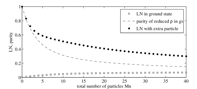
Figure 2: Entanglement (as measured by the logarithmic negativity ${\rm LN}$) between the outer sites for the superfluid ground state (squares) and the superfluid ground state with an extra particle using $c_{i}=(\delta_{i1}+\delta_{iM})/\sqrt{2}$ (filled circles) as discussed in the text. The number of sites is $M=20$. The purity $\rm{tr}[(\hat{\rho}_{\rm SF})^{2}]$ of the reduced density matrix is plotted as a dashed line. For the insulator case (with integer $\bar{n}$), always ${\rm LN}(\hat{\rho}^{\prime}_{{\rm MI},\bar{n}})=0$ for the ground state and ${\rm LN}(\hat{\rho}^{\prime}_{{\rm MI},\bar{n}})=1$ for the ground state with an additional particle and $c_{i}$ as above.

In order to discuss the entanglement generated from an extra particle on top of the ground state, let us consider the simplified situation $c_{i}=(\delta_{i1}+\delta_{iM})/\sqrt{2}$. For the Mott case,

$$\hat{\rho}^{\prime}_{\rm MI,\bar{n}}=\frac{1}{4}\left(|\bar{n}+1,\bar{n}\rangle+|\bar{n},\bar{n}+1\rangle\right)\left(\langle\bar{n}+1,\bar{n}|+\langle\bar{n},\bar{n}+1|\right),$$ (22)

which is a pure state with logarithmic negativity ${\rm LN}(\hat{\rho}^{\prime}_{{\rm MI},\bar{n}})=1$, independently of $\bar{n}$. Note that the entanglement is completely contained in the sector of $2\bar{n}+1$ particles shared between the outer sites. This is different for the superfluid phase. Here the extra particle on top of the ground state with filling factor $\bar{n}$ leads to

$$\hat{\rho}^{\prime}_{\rm SF,\bar{n}}=\sum_{k=0}^{M\bar{n}+1}(\gamma^{\prime}_{k})^{2}|\phi_{\rm SF}^{\,k}\rangle\langle\phi_{\rm SF}^{\,k}|,$$ (23)

with $\gamma^{\prime}_{0}=0$, and

$$(\gamma^{\prime}_{k})^{2}=\frac{k(\gamma_{k-1})^{2}}{1+2\bar{n}}\quad\textrm{for}\quad k>0.$$ (24)

Clearly, for an empty lattice, $\bar{n}=0$, the choice of $c_{i}$ leads to ${\rm LN}(\hat{\rho}^{\prime}_{{\rm SF},\bar{n}=0})=1$. For $\bar{n}>0$, the logarithmic negativity $\hat{\rho}^{\prime}_{\rm SF}$ decreases (Fig. 2). Again, as $\bar{n}$ grows the number of degrees of freedom which potentially can be entangled increases also. Still, in this case the two outer sites are less entangled due to the smaller purity of the reduced density matrix (the outer sites are more entangled to the inner part of the chain). It might seem counter-intuitive that

$${\rm LN}(\hat{\rho}^{\prime}_{\rm SF,\bar{n}})<{\rm LN}(\hat{\rho}^{\prime}_{\rm SF,\bar{n}=0}),$$ (25)

despite the additivity property of the logarithmic negativity [24]. Here we should again remark, that the occupation number basis which is used to quantify entanglement does not reflect the tensor product structure of individual particles. In fact, the bosonic particles themselves live in a symmetrized subspace which does not have the structure of a full tensor product (this indeed is the reason why for bosonic particles new measures of entanglement have to be introduced).

Let us finally note that if the systems dynamics is governed by the Bose-Hubbard Hamiltonian, then the logarithmic negativity will always be below the values of Fig. 2, as in this case the $c_{i}(t)$’s are given by Eq. (8).

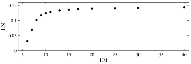
Figure 3: Entanglement between the two outer sites of the lattice, measured by the logarithmic negativity ${\rm LN}(\hat{\rho}_{1M})$, versus $U/J$ for a chain of $M=41$ sites (after inserting an extra particle at site at $(M+1)/2$). The chemical potential $\mu$ is adapted to have a ground state with mean number of particles per site $\bar{n}=1$ ($\mu=U/(2J)$ for $U\gg J$). The data is obtained through MPS simulations truncating the basis to states of up to $5$ particles per site and using $D\leq 20$.

To study how the competition between interactions and tunneling affects the generation of entanglement when adding an extra particle, we numerically calculate time evolution of the initial state for a wide range of parameters, $6<U/J<40$. We use standard numerical MPS algorithms [25]. As we limit the number of particles per site to $5$ in our simulations, we cannot study states well inside the superfluid regime, where for $\bar{n}=1$ up to $M$ particles per site have to be taken into account. Still, already for values of $U/J<15$ drastic changes due to the possibility of tunneling are manifested in the entanglement between the outer lattice sites. To calculate $|\psi(t)\rangle=\exp(-{\rm i}\hat{H}_{\rm BH}t)|\psi^{\bar{n}=1}_{GS}\rangle$, we first obtain the ground state of the Bose-Hubbard Hamiltonian for different values of the parameter $U/J$. We choose the chemical potential as $\mu/J=U/(2J)$ in the case of large $U/J$. For small values of the ratio $U/J$, we adjust $\mu$ appropriately, in order to obtain the ground state $|{\Psi}^{\bar{n}=1}_{GS}\rangle$ with filling factor $\bar{n}=1$. Having the ground state, we add a particle to the system and obtain the dynamics through a time-dependent MPS simulations. From the MPS state, the reduced density matrix $\hat{\rho}_{1,M}$ of the outer sites can be extracted efficiently, such that we can compute the logarithmic negativity as a function of time. In Fig. 3 we display the value of ${\rm LN}(\hat{\rho}_{1,M})$ at its first maximum as a function of $U/J$. In Fig. 4 we analyze time evolution in detail for two cases: well in the MI phase ($U/J=40$) and close to the SF phase ($U/J=6$). Figs. 4 (a,c) show the propagation of the excitation, i.e., the mean occupation number $\langle n_{i}\rangle$ versus time. The propagation in the two cases is very similar (as it is visible from the figures, the evolution is slower for $U/J=6$, though not by a factor of $2$ as it would be the case for $U/J=0$). The propagation of entanglement, visualized in Figs. 4 (b,d) through the logarithmic negativities of the reduced density matrices of sites $(M-1)/2\pm k$, is different in the two cases. Clearly, the efficient generation of entanglement in the occupation number basis requires a Mott insulator background. As we demonstrated, entanglement generation is much less efficient if tunneling becomes comparable to or larger than interactions.

A strategy to increase entanglement in a system of ideal (interactionless) bosons in the occupation number basis consists in loading several bosons in a given site of an otherwise empty lattice [14]. For interacting particles, however, in the limit $U\gg J$, entanglement does not increase if all $N$ particles are initially located at the same site. In this case, tunneling of a single particle alone is strongly suppressed and atoms tunnel together. Treating the tunneling term perturbatively, it can be seen that the evolution is slower by a factor $J/(UN)$.

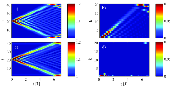
Figure 4: Left column: mean ocupation number $n_{i}=\langle\hat{n}_{i}\rangle$ of site $i$ as a function of time for a chain of $M=41$ lattice sites ((a) $U/J=40$; (c) $U/J=6$). The system is initially cooled to its ground state with filling factor $\bar{n}=1$. At $t=0$, a further particle is loaded at site $i=20$. Right column: logarithmic negativity ${\rm LN}(\hat{\rho}_{21-k,21+k})$ of the reduced density matrix of sites $21-k$ and $21+k$, $k=1,\ldots,20$ versus time for (b) $U/J=40$, (d) $U/J=6$.

3 Creating entangled “spatially delocalized quantum bits”

In this section we discuss an alternative way of defining a quantum bit in a lattice filled with spinless bosons. This definition does not rely on the occupation number basis, leading to a notion of entanglement which is physically more sound. We use the concept of “spatially delocalized quantum bits” (SDQs), in which the binary alternative consists in having an atom either in one side or in the adjacent one.

To be specific, we use a single particle shared between two (adjacent) sites $i,\,i+1$ of the chain to define a quantum bit by identifying $|0\rangle_{\rm SDQ}\equiv|n_{i}=1,n_{i+1}=0\rangle$ and $|1\rangle_{\rm SDQ}\equiv|n_{i}=0,n_{i+1}=1\rangle$. Though in this definition again a qubit is defined via absence or presence of a particle on a lattice site, now one particle is necessary per qubit. In this way, for any unitary transformation the number of particles is conserved locally. For such “charge” or “spatially delocalized” qubits, implementations of quantum gates have been proposed for bosonic atoms in optical lattices [27], as well as for electrons in quantum dots [28] or photons in photonic crystals [29].

To entangle two such qubits at the ends of a 1D chain of even length $M$, we place two particles at sites $M/2$ and $M/2-1$ (in the middle of the chain) and let the system evolve. As before, we start by considering an otherwise empty chain, i.e., the quantum walk with two particles: $|\psi(t=0)\rangle=\hat{a}^{{\dagger}}_{M/2}\hat{a}^{{\dagger}}_{M/2+1}|\Omega\rangle$. For a spatially delocalized qubit defined through a particle shared between sites $i,j$, we introduce the corresponding projection operators $\hat{P}^{(i,j)}_{\alpha}=|\alpha\rangle_{\rm SDQ}\langle\alpha|$. For instance,

$$\hat{P}^{(i,j)}_{0}=|0\rangle_{\rm sdq\!}\langle 0|=|n_{i}=1,n_{j}=0\rangle\langle n_{i}=1,n_{j}=0|.$$ (26)

$\hat{P}_{0}^{(i,j)}+\hat{P}_{1}^{(i,j)}$ thus projects onto the subspace having a single particle shared between sites $i$ and $j$. If two qubits are defined on sites $(1,2)$ and $(M-1,M)$ respectively, we obtain the density matrix for the two spatially delocalized qubits as

$$\hat{\rho}^{\rm sdq}_{\alpha\beta,\alpha^{\prime},\beta^{\prime}}(t)=\hat{P}^{(1,2)}_{\alpha}\otimes\hat{P}^{(M-1,M)}_{\beta}|\psi(t)\rangle\langle\psi(t)|\hat{P}^{(1,2)}_{\alpha^{\prime}}\otimes\hat{P}^{(M-1,M)}_{\beta^{\prime}}.$$ (27)

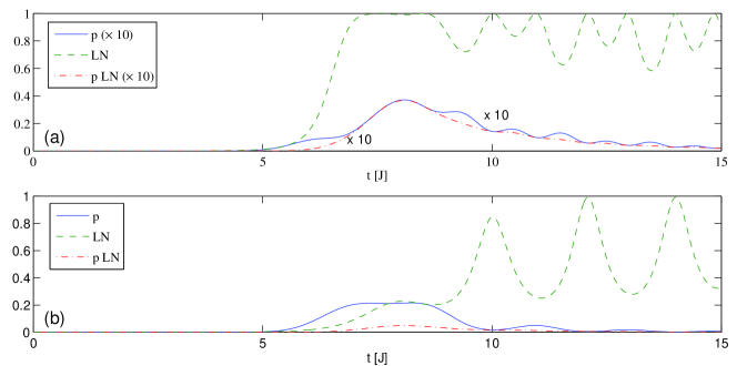
Figure 5: Probability $p$ for the successful projection onto the subspace of one particle per spatially delocalized qubit (straight blue line) , logarithmic negativity ${\rm LN}$ (dashed green line) between the qubits after successful projection, and the product $p\;{\rm LN}$ (dashed red line) for a chain of $24$ sites with (a) no interaction $U/J=0$ and (b) strong interaction $U/J=20$. Results from MPS simulations with $D=18$.

The probability $p$ of a successful projection onto the subspace of one particle per SDQ is given by $p=\tr{\hat{\rho}^{\rm sdq}}\leq 1$, and the entanglement between the two spatially delocalized qubits in case of a successful projection is measured by the logarithmic negativity of the correctly normalized state ${\rm LN}(\hat{\rho}^{\rm sdq}/p)$. The probability $p$, the logarithmic negativity ${\rm LN}$, and the probabilistic entanglement $p\;{\rm LN}$ are plotted in Fig. 5 (a) for the case of no interaction between the two bosons ($U/J=0$) and for strong interaction between them ($U/J\gg 1$) in Fig. 5 (b).

The time-dependence of the logarithmic negativity, as well as of the probability $p$, is clearly different in the two cases. It is illustrative to consider the case of only four sites, (with the two particles initially located at sites $2$ and $3$). Then the initial state is $|10\rangle_{\rm SDQ}$, which is a separable state of the two spatially delocalized qubits. If interactions are absent, then already at early times populations of states lying in the delocalized qubit space can originate from two possible paths (starting at sites $2$ or $3$, respectively). It is this interference which leads to a fast generation of entanglement. If interactions are strong, then one of this paths is effectively suppressed at early times as each particle is confined to “its” qubit (this leads to the larger probability $p$ for a successful projection). Entanglement in this case is (initially) only generated through the collisional phase shift (this effect can be used to implement a phase gate for spatially delocalized qubits [27]), which however is small. As a consequence, entanglement is smaller if interactions are large.

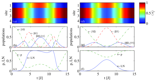
Figure 6: Generation of entanglement between two spatially delocalized qubits formed from sites $1,\,2$ and $3,\,4$, respectively. Left column: $U/J=0$, right column: $U/J=20$. (a,d) show the mean site occupation $\langle n_{i}\rangle$, (b,e) the populations ${}_{\rm SDQ}\langle\alpha\beta|\hat{\rho}^{\rm SDQ}(t)/p|\alpha\beta\rangle_{\rm SDQ}$, and (c,f) give the probability $p$ of successful projection into the subspace of one particle per spatially delocalized qubit and the entanglement measured via the logarithmic negativity ${\rm LN}$.

In the presence of a ground state background with an average number $\bar{n}$ of particles per site, generating (entangled) spatially delocalized quantum bits from the evolution of two extra particles only can be done effectively in the Mott case. Here the definition of the basis can be modified as $|0\rangle_{\rm SDQ}\equiv|n_{i}=\bar{n}+1,n_{i+1}=\bar{n}\rangle,\,|1\rangle_{\rm SDQ}\equiv|n_{i}=\bar{n},n_{i+1}=\bar{n}+1\rangle$. In the superfluid case, the on-site particle number fluctuations in the ground state require a projection onto the subspace of fixed number of particles per spatially delocalized qubit, which strongly reduces the efficiency of the scheme.

4 Conclusions

Summarizing, we have analyzed the generation of entanglement between the outer extremes of a 1D Bose-Hubbard chain by loading an extra particle on top of the ground state. We have investigated effects arising from direct competition between tunneling and interactions in the entanglement behavior. In some limiting cases, the bosonic propagation can be adequately described as continuous time quantum walks. As part of our analysis, we have discussed two conceptually different “computational bases” to quantify entanglement between particles which have no internal degrees of freedom, namely the occupation number basis and a spatially delocalized qubit basis.

References

References

- [1] C.H. Bennett and D.P. DiVincenzo. Quantum information and computation. Nature, 404:247, March 2000.
- [2] S. Bose. Quantum communication through an unmodulated spin chain. Phys. Rev. Lett., 91(20):207901, 2003.
- [3] M. Christandl, N. Datta, A. Ekert, and A.J. Landahl. Perfect state transfer in quantum spin networks. Phys. Rev. Lett., 92(18):187902, 2004.
- [4] O. Romero-Isart, K. Eckert, and A. Sanpera. Quantum state transfer in spin-1 chains: Uncovering the magnetic order. quant-ph/0610210.
- [5] T.S. Cubitt and J.I. Cirac. Engineering correlation and entanglement dynamics in spin systems. quant-ph/0701053.
- [6] S. Montangero, G. Benenti, and R. Fazio. Dynamics of Entanglement in Quantum Computers with Imperfections. Phys. Rev. Lett. 91:187901, 2003.
- [7] J. Vidal, G. Palacios, and C. Aslangul. Entanglement dynamics in the Lipkin-Meshkov-Glick model. Phys. Rev. A 70:062304, 2004.
- [8] L. Amico, A. Osterloh, F. Plastina, R. Fazio, and G. Massimo Palma. Dynamics of entanglement in one-dimensional spin systems. Phys. Rev. A 69:022304, 2004.
- [9] M. Lewenstein, A.Sanpera, V. Ahufinger, B. Damski, A. Sen De, and U. Sen. Ultracold atomic gases in optical lattices: Mimicking condensed matter physics and beyond. cond-mat/0606771.
- [10] F.D.M. Haldane. Solidification in a soluble model of bosons on a one-dimensional lattice: The Boson-Hubbard chain. Phys. Lett. A 80:281, 1980.
- [11] M.P.A. Fisher, P.B. Weichman, G. Grinstein, and D.S. Fisher Boson localization and the superfluid-insulator transition Phys. Rev. B 40:546, 1989.
- [12] D. Jaksch, C. Bruder, J.I. Cirac, C.W. Gardiner, and P. Zoller. Cold bosonic atoms in optical lattices. Phys. Rev. Lett., 81:3108, 1998.
- [13] M. Greiner, O. Mandel, T. Esslinger, T.W. Hänsch, and I. Bloch. Quantum phase transition from a superfluid to a mott insulator in a gas of ultracold atoms. Nature, 415:39, 2002.
- [14] S. Bose. Entanglement from the dynamics of an ideal bose gas in a lattice. cond-mat/0610024.
- [15] S. L. Cornish, N. R. Claussen, J. L. Roberts, E. A. Cornell, and C. E. Wieman. Stable bose-einstein condensates with widely tunable interactions. Phys. Rev. Lett., 85(9):1795–1798, Aug 2000.
- [16] T.D. Kühner, S.R. White, and H. Monien. One-dimensional bose-hubbard model with nearest-neighbor interaction. Phys. Rev. B, 61:12474, 2000.
- [17] J. Kempe. Quantum random walks: an introductory overview. Cont. Phys., 44:307, 2003.
- [18] A. Childs, E. Farhi, and S. Gutmann. An example of the difference between quantum and classical random walks. Quantum Information processing, 1:35, 2002.
- [19] P. Zanardi. Quantum entanglement in fermionic lattices. Phys. Rev. A, 65:042101, 2002.
- [20] J.R. Gittings and A.J. Fisher. Describing mixed spin-space entanglement of pure states of indistinguishable particles using an occupation number basis. Phys. Rev. A, 66:032305, 2002.
- [21] Y. Omar, N. Paunkovic, S. Bose, and V. Vedral. Spin-space entanglement transfer and quantum statistics. Phys. Rev. A, 65:062305, 2002.
- [22] C. Simon. Natural entanglement in Bose-Einstein condensates. Phys. Rev. A, 66:052323, 2002.
- [23] Y. Shi. Quantum entanglement of identical particles. Phys. Rev. A, 67:024301, 2003.
- [24] M.B. Plenio and S. Virmani. An introduction to entanglement measures. Quant. Inform. Comp., 7:1, 2007.
- [25] J.J. Garcia-Ripoll. Time evolution algorithms for Matrix Product States and DMRG. New J. Physics 8:305, 2006.
- [26] J.k. Freericks and H. Monien. Strong-coupling expansions for the pure and disordered Bose-Hubbard model. Phys. Rev. B 53:2691, 1996,
- [27] J. Mompart, K. Eckert, W. Ertmer, G. Birkl, and M. Lewenstein. Quantum computing with spatially delocalized qubits. Phys. Rev. Lett., 90:147901, 2003.
- [28] F. Renzoni and T. Brandes. Charge transport through quantum dots via time-varying tunnel coupling. Phys. Rev. B, 64:245301, 2001.
- [29] D.G. Angelakis, M.F. Santos, V. Yannopapas, and A. Ekert. Quantum computation in photonic crystals. quant-ph/0410189.