Abstract

In view of the current discussion on the subject, an effort is made to show very accurately both analytically and numerically how the Drude dispersion model gives consistent results for the Casimir free energy at low temperatures. Specifically, for the free energy near $T=0$ we find the leading term proportional to $T^{2}$ and the next-to-leading term proportional to $T^{5/2}$. These terms give rise to zero Casimir entropy as $T\rightarrow 0$, and is thus in accordance with Nernst’s theorem.

PACS numbers: 05.30.-d, 12.20.Ds, 42.50.Nn, 65.40.Gr

1 Introduction

In recent years there has been a lively discussion about the thermodynamic consistency of the expression for the Casimir pressure at finite temperature $T$. The problem gets accentuated at low values of $T$, where one has to satisfy the Nernst theorem saying that $S=-\partial F/\partial T$ goes to zero as $T\rightarrow 0$. (Here $S$ is the entropy and $F$ the free energy, both referring to unit plate area.) What we shall consider in the following is the standard Casimir configuration, implying two semi-infinite homogeneous metallic media separated by a vacuum gap of width $a$. We take the two media to be identical, and assume that they are nonmagnetic with a frequency dependent relative permittivity $\varepsilon(\omega)$. Spatial dispersion is neglected. The two surfaces lying at $z=0$ and $z=a$ are assumed to be perfectly plane, and to be of infinite extent.

A central ingredient in the discussion of the thermodynamic consistency of calculated results for the Casimir attractive force between real materials is the form of dispersion relation used as input in the conventional Lifshitz formula. A very useful dispersion relation - the one that in our opinion is by far the most preferable one amongst simple dispersion relations for real systems at arbitrary frequencies - is the Drude expression

$$\varepsilon(i\zeta)=1+\frac{\omega_{p}^{2}}{\zeta(\zeta+\nu)}.$$ (1)

Here $\omega=i\zeta$, $\omega_{p}$ is the plasma frequency, and $\nu$ is the relaxation frequency (we use the same notation as in Ref. [1]). The plasma wavelength is $\lambda_{p}=2\pi c/\omega_{p}$. For gold, the substance that we shall focus on in the following, we use

$$\omega_{p}=9.03\,{\rm eV},\quad\nu=34.5\,{\rm meV},\quad\lambda_{p}=137.4\,{\rm nm}.$$ (2)

In Ref. [1], we employed the values $\omega_{p}=9.0$ eV, $\nu=35$ meV, what amounts roughly to a difference on the 1% level. The exact determination of Drude parameters is a non-trivial matter as discussed in [2]. Using a slightly different set of Drude parameters will shift our numerical results slightly, but does not alter any of our conclusions.

When comparing with experimental values it turns out that the Drude relation fits optical data very accurately for $\zeta<2\times 10^{15}$ rad/s [3, 4]. In this connection we should bear in mind the following fact (cf. also the discussion in Ref. [5]): There exist no measurements of the permittivity at very low frequencies. What is available, is a series of measurements of the imaginary part $\varepsilon^{\prime\prime}(\omega)$ of the complex permittivity $\varepsilon(\omega)=\varepsilon^{\prime}(\omega)+i\varepsilon^{\prime\prime}(\omega)$. The Kramers-Kronig relations then permit us to calculate the real part $\varepsilon^{\prime}(\omega)$, and thus the complete $\varepsilon(\omega)$ is known. Permittivity data kindly supplied by Astrid Lambrecht cover a very large frequency region, from $1.5\times 10^{11}$ rad/s to $1.5\times 10^{18}$ rad/s. From these data, the relaxation frequency $\nu$ can be derived. As mentioned, from comparison with experimental data it turns out that $\nu$ can be taken to be constant to a good accuracy, up to about $\zeta=2\times 10^{15}$ rad/s. For low frequencies the Drude relation yields the proper extrapolation down to $\zeta=0$.

A word of caution is called for, as regards the circumstance that permittivity measurements are done at room temperature in practice. The frequency $\nu$ is in principle temperature dependent, and we do not know the value of $\nu(T=0)$ very accurately. It might seem natural here to invoke the Bloch-Grüneisen formula for the temperature dependence of the electrical resistivity (cf. [6] or also the discussion in Ref. [1]). From this, a form for $\nu=\nu(T)$ can in principle be found. According to the formula, the value of $\nu$ should go to zero as $T\rightarrow 0$. However, in practice this is not true. There are always impurities present, which make the value of $\nu$ finite at $T=0$ [7]. The Bloch-Grüneisen formula, thus, is not followed in this limit. Mathematically, the important point is that

$$\zeta^{2}[\varepsilon(i\zeta)-1]\rightarrow 0\quad{\rm as}\quad\zeta\rightarrow 0.$$ (3)

This relation ensures that the zero-frequency transverse electric (TE) mode does not contribute to the Casimir force at all, as discussed in detail in Ref. [1]. Strictly, the Drude parameters of Eq. (2) are valid at room-temperature, and $\nu$ will take significantly smaller values for low temperatures. This affects our numerical results quantitatively, but not qualitatively; as long as $\nu$ is nonzero, the TE part of the free energy vanishes at zero frequency which is the central point.

The recent series of works on the Casimir effect by the present group of authors [1, 8, 9, 10, 5, 11, 12, 13] - built upon the Lifshitz formula and the measured values of $\varepsilon(\omega)$ in combination with the Drude relation - have nowhere been found to run into conflict with basic thermodynamic principles. And there are other papers in agreement with ours: for instance, Jancovici and Šamaj [14], and Buenzli and Martin [15] considered the Casimir force between two plates in the high-temperature limit. They found that the linear dependence in $T$ for the Casimir force to be reduced by a factor of two from the behavior of of an ideal metal, this being a signal of the vanishing influence from the zero-frequency TE mode. (The first observation of the vanishing influence from this particular mode was made by Boström and Sernelius [16].) Further support is found in the paper of Sernelius [17], who calculates the Casimir force taking spatial dispersion into account as well. It is found that at high temperatures and/or at large separations the force is reduced by the same factor of two compared with the ideal-metal result.

There is no universal agreement on these issues, however. In a series of recent papers - cf., for instance, Refs. [18, 19, 20, 21, 22] - it is argued that the Drude dispersion relation runs into trouble explaining recent experiments, and moreover comes into conflict with the Nernst theorem. These authors favor, instead of the Drude relation, the plasma relation

$$\varepsilon(i\zeta)=1+\frac{\omega_{p}^{2}}{\zeta^{2}},$$ (4)

which corresponds to setting $\nu=0$ in Eq. (1). (It should be noted that the expression (4) does not satisfy the condition (3).)

An argument of the latter references is that omission of a zero frequency TE-mode would add a term linear in $T$ to the free energy. This would violate the Nernst theorem as it would give a non-zero contribution to the entropy at $T=0$. However, this argument is based upon use of the IM (idealized metal) model where $\varepsilon=\infty$ for all $\zeta$, or use of the plasma model (4) where no relaxation is present. With $\nu>0$ the term in question is still linear away from $T=0$, but the precise behavior as $T\rightarrow 0$ has been less obvious. As argued in Ref. [1] the straight line should bend to become horizontal at $T=0$. This was not verified in utmost detail, however; the numerical results of Ref. [1] did not go sufficiently close to $T=0$ to show the behavior very distinctly, and the previous discussion and disagreement about violation of the Nernst theorem has accordingly continued. The main purpose of the present work is to investigate the issue more closely: we will show in detail, both analytically and numerically, how the Casimir energy behaves close to $T=0$ and by that show how it is consistent with the Nernst theorem.

We shall not go into a study of experimental aspects in this paper. Rather, the objections referred to above makes it mandatory to reconsider the thermodynamics associated with the Drude relation anew, which brings us to the central theme of this paper. We will aim at showing, via a combination of analytical and numerical methods, how the basic theory sketched above (essentially the Drude theory) satisfies the Nernst theorem to a very high accuracy. We consider this point to be important; a simple physical model of course cannot be permitted to run into conflict with thermodynamics.

In the next section we show analytically, by using the Euler-Maclaurin formula, that the dominant contribution to the free Casimir energy $F$ near $T=0$ is proportional to $T^{2}$. We evaluate both this term and the leading correction term, which is proportional to $T^{5/2}$. This implies that the entropy $S=-\partial F/\partial T$ tends to zero as $T\rightarrow 0$, in accordance with the Nernst theorem. In Sect. 3 we calculate $F$ numerically, and find agreement with the previous analytical result to a very high degree of accuracy. The results are illustrated in various figures. Thus we can conclude that the Drude ansatz does not run into conflict with thermodynamics at all.

Readers interested in recent reviews on the Casimir effect may consult Milton’s book [23], and several review articles [24, 25, 26, 27]. A great deal of recent information can also be found in the special issues of J. Phys. A: Math. Gen. [28] and of New J. Phys. [29].

As mentioned above, we shall not be concerned with comparison between theory and experiment in the present paper. We mention, though, the recent experiment of Obrecht et al. [30], which seems to report the first accurate measurement of thermal Casimir effects. The experiment is important, but it lies outside the scope of the present investigation since it deals with non-uniformly heated systems.

Finally, we mention the special variant of the thermal Casimir problem consisting in studying, instead of a metal, a semiconductor endowed with a small but finite conductivity at zero frequency [31, 32]. According to the authors of these references this situation implies an interchange of the roles of the TE and TM (transverse magnetic) modes, as compared with the case of a metal. Namely, within an idealized approach, they find that the TM reflection coefficient gets a discontinuity at $\zeta=0$, implying in turn an apparent conflict with the Nernst theorem. The problem is interesting, and we hope to return to it in a later paper.

2 Analytical approach: Casimir free energy near $T=0$ for real metals

As mentioned, we use the same notation as in Ref. [1]. We will evaluate the leading $T$-dependence of the Casimir free energy near $T=0$ for metals using the Drude relation (1),

$$\varepsilon(i\zeta)-1=\frac{\omega_{p}^{2}}{\zeta(\zeta+\nu)}\approx\frac{D}{\zeta},\quad{\zeta\ll\nu},$$ (5)

with $D=\omega_{p}^{2}/\nu$. The free energy is given by expression (3.4a) in [1] as

$$\beta F=\frac{1}{2\pi}{\sum\limits_{m=0}^{\infty}}^{\prime}\int\limits_{\zeta/c}^{\infty}[\ln(1-\lambda^{\mathrm{TM}})+\ln(1-\lambda^{\mathrm{TE}})]qdq$$ (6)

where $\beta=1/kT$ and

$$\lambda^{\mathrm{TM}} = Ae^{-2qa},$$

$$\lambda^{\mathrm{TE}} = Be^{-2qa}.$$

The prime on the summation sign means that the case $m=0$ is taken with half weight. The coefficients $A$ and $B$ are the squared Fresnel reflection coefficients for the two media and are given by

$$A=\left(\frac{s-\epsilon p}{s+\epsilon p}\right)^{2},\quad B=\left(\frac{s-p}{s+p}\right)^{2},$$ (7)

with

$$s=\sqrt{\varepsilon-1+p^{2}},\quad p=\frac{qc}{\zeta}.$$

Here $a$ is the plate separation, $\varepsilon$ the relative permittivity, $c$ the velocity of light in vacuum, and $\zeta$ is the Matsubara frequency given by

$$\zeta=\frac{2\pi k}{\hbar}mT.$$ (8)

Note that the quantities of $A,B,s,p$ and $\zeta$ all depend upon the summation variable $m$. (Units $c=\hbar=k=1$ are not used.) The term of interest is the TE mode, since this is the term that gives rise to the controversy about the Nernst theorem.

With the small $\zeta$ dependence of Eq. (5) the $B$ has a scaling form such that it can be expressed in terms of one variable. So by introducing a new variable $x$ to replace $q$ the $\zeta$-dependence can be removed fully

$$x^{2}=\frac{q^{2}c^{2}}{(\varepsilon-1)\zeta^{2}}\approx\frac{q^{2}c^{2}}{D\zeta},\quad\zeta\ll\nu.$$ (9)

With this we have

$$B=\left(\frac{\sqrt{1+x^{2}}-x}{\sqrt{1+x^{2}}+x}\right)^{2}=(\sqrt{1+x^{2}}-x)^{4},$$ (10)

and the TE free energy expression can be written as

$$\beta F^{TE}=C{\sum\limits_{m=0}^{\infty}}^{\prime}g(m),$$ (11)

with

$$g(m)=m\int_{x_{0}}^{\infty}x\ln{(1-Be^{-y})}\,dx,$$ (12)

where

$$C=\frac{D}{c^{2}\hbar\beta}=\frac{\omega_{p}^{2}}{c^{2}\hbar\nu\beta},\quad y=2qa=2\frac{a}{c}\sqrt{D\zeta}\,x,\quad x_{0}=\sqrt{\frac{\zeta}{D}}.$$ (13)

The small $T$-behavior can now be obtained by use of the Euler-Maclaurin summation formula

$${\sum_{n=0}^{\infty}}^{\prime}g(n)=\int\limits_{0}^{\infty}g(u)\,du-\frac{1}{12}g^{\prime}(0)+\frac{1}{720}g^{\prime\prime\prime}(0)-...$$ (14)

One easily sees that

$$g^{\prime}(0)=\int_{0}^{\infty}x\ln{(1-B)}\,dx.$$ (15)

This integral can be performed analytically. First introduce a new variable $x=\sinh t$ with $dx=\cosh t\,dt$

$$g^{\prime}(0)=\int\limits_{0}^{\infty}\sinh t\,\cosh t\,\ln(1-e^{-4t})\,dt=\frac{1}{4}\int\limits_{0}^{\infty}(e^{2t}-e^{-2t})\ln(1-e^{-4t})\,dt.$$ (16)

Next we substitute $e^{-2t}=u$ for which $-2e^{-2t}\,dt=du$ and use partial integration to obtain

$$g^{\prime}(0) = -\frac{1}{8}\int\limits_{0}^{1}\left(1-\frac{1}{u^{2}}\right)\ln(1-u^{2})\,du$$ (17)

$$= -\frac{1}{8}\left\{\frac{1}{u}[(1+u)^{2}\ln(1+u)+(1-u)^{2}\ln(1-u)]-2u\right\}_{0}^{1}$$

$$= -\frac{1}{4}(2\ln 2-1)\approx-0.09657.$$

At $T=0$ the free energy is determined by the integral in Eq. (14) (besides contribution from the TM-mode). For small $T\rightarrow 0$ the deviation from the $T=0$ value is thus ($\beta=1/kT$)

$$\Delta F^{TE}=\frac{C}{\beta}\left[-\frac{1}{12}g^{\prime}(0)\right]=\frac{C}{48\beta}(2\ln 2-1).$$ (18)

This result was presented by Milton at the QFEXT03 Workshop, and is given as Eq. (22) in Ref. [8], or Eq. (4.9) in Ref. [11].

It can be noted that $\Delta F^{TE}$ is independent of the plate separation $a$ and can thus be valid only sufficiently close to $T=0$ for a given $a$ such that $\Delta F^{TE}\ll F^{TE}\sim\hbar c/a^{3}$. Evaluation of the next term as given by result (30) below verifies this. The leading term of $\Delta F^{TE}$ dominates its next term only when the dimensionless quantity $aC^{1/2}\ll 1\;$ or $a^{2}kT\ll\hbar\nu c^{2}/\omega_{p}^{2}$. A consequence of this is that for increasing $a$ the temperature interval where (18) is valid decreases rapidly, and $\Delta F^{TE}$ becomes more and more negligible compared to $F^{TE}$ since then $\Delta F^{TE}\sim C/\beta=\omega_{p}^{2}(kT)^{2}/(c^{2}\hbar\nu)\ll c^{2}\hbar\nu/(\omega_{p}^{2}a^{4})$. (Thus in the present case $\Delta F^{TE}\ll F^{TE}$ provided $a>c\nu/\omega_{p}^{2}\approx 0.1$ nm with $a^{2}kT\ll\hbar\nu c^{2}/\omega_{p}^{2}$ fulfilled.) In the limit $a\rightarrow\infty$ the IM ($\varepsilon=\infty$), but now with the linear term included, is recovered. But the latter does not violate the Nernst theorem as long as $a$ is finite, and for $a=\infty$ there is no Casimir free energy anyway.

Inserting the value for $g^{\prime}(0)$ and the values $\hbar\omega_{p}=9.03$ eV and $\hbar\nu=34.5$ meV for Au we find with $C$ given by (13) ($\hbar=1.0545\cdot 10^{-34}$ Js, $k=1.381\cdot 10^{-23}$ J/K, $c=2.998\cdot 10^{8}$ m/s)

$$\Delta F^{TE}=C_{1}T^{2}\quad\mbox{with}\quad C_{1}\approx 5.81\cdot 10^{-13}\,\mbox{J/(m}^{2}{\rm K}^{2}).$$ (19)

It turns out that Eq. (18) holds only very close to $T=0$ (i. e. $T\ll 0.01$ K), but there will be a leading correction that we can obtain with good accuracy. Expanding $g(m)$ in powers of $m$ one notes that half integer powers will occur. Thus formula (14) is not quite valid as $g^{\prime\prime\prime}(0)$ and higher order derivatives will diverge. However, this problem can be avoided since the formula can be applied to summation starting at $m=p$ ($p=1,2,3,\cdots$). Thus we have

$$\sum_{n=0}^{\infty}g(n) = \sum_{n=0}^{p-1}g(n)+\int\limits_{p}^{\infty}g(u)\,du+\frac{1}{2}g(p)-\frac{1}{12}g^{\prime}(p)+\frac{1}{720}g^{\prime\prime\prime}(p)+\cdots$$ (20)

$$= \int\limits_{0}^{\infty}g(u)\,du+S-\frac{1}{12}g^{\prime}(p)+\frac{1}{720}g^{\prime\prime\prime}(p)+\cdots$$

where

$$S=\sum_{n=0}^{p-1}g(n)+\frac{1}{2}g(p)-\int\limits_{0}^{p}g(u)\,du.$$ (21)

For a power term $g_{\sigma}(m)=m^{\sigma}$ (for small $m$) we have

$$g^{\prime}_{\sigma}(p)=\sigma p^{\sigma-1},\quad g^{\prime\prime\prime}_{\sigma}(p)=\sigma(\sigma-1)(\sigma-2)p^{\sigma-3},\quad\int\limits_{0}^{p}g_{\sigma}(u)\,du=\frac{1}{1+\sigma}p^{\sigma+1}.$$ (22)

With the choice $p=1$ we get

$$S=S_{\sigma}(1)=\frac{1}{2}-\frac{1}{1+\sigma}.$$ (23)

One may note that $S_{1}(1)=0$ as should be expected. The power of key interest here will be $\sigma=3/2$ by which $S_{\sigma}=1/10$ , and thus

$$\Delta S_{\sigma}(1)\equiv S_{\sigma}(1)-\frac{1}{12}g^{\prime}_{\sigma}(1)+\frac{1}{720}g^{\prime\prime\prime}_{\sigma}(1)\approx-0.02552\approx-0.204\frac{1}{12}g^{\prime}_{\sigma}(1).$$ (24)

When other terms are neglected the error can be estimated from the next term in the series (provided the sum of higher order terms converge)

$$\frac{1}{30240}g^{(V)}_{\sigma}(1)=\frac{-1}{30240}\,\frac{3}{2}\left(\frac{1}{2}\right)\left(\frac{-1}{2}\right)\left(\frac{-3}{2}\right)\left(\frac{-5}{2}\right)\approx 4.65\cdot 10^{-5},$$ (25)

which is only about 0.2% of the value (24). For increasing values of $p$ the error goes further down rapidly. (Instead of result (24) $p=2$ yields $\approx-0.02549$.) Thus (24) with $p=1$ is a good estimate for the sum of interest.

With $g(m)$ given by (12) we can expand to leading order in $m$ or $y~{}(\propto T^{1/2})$. To this leading order the limit of integration $x_{0}~{}(\propto T^{1/2})$ can be put equal to zero since the integrand vanishes for $x=0$. We find

$$g(m)=mg^{\prime}(0)+myI+\cdots$$ (26)

Now from (8) and (13)

$$y=2a\sqrt{2\pi C}xm^{1/2},$$ (27)

with $C$ given by (13). Thus the derivative becomes

$$g^{\prime}(m)=g^{\prime}(0)+3a\sqrt{2\pi C}\,Im^{1/2}+\cdots$$ (28)

where $g^{\prime}(0)$ is given by (17) and (with substitution $x=\sinh t$ as in (16))

$$I=\int\limits_{0}^{\infty}\frac{x^{2}B}{1-B}\,dx=\frac{1}{8}\int\limits_{0}^{\infty}(e^{-t}-e^{-3t})\,dt=\frac{1}{12}.$$ (29)

Now we will use Eq. (21) for the most simple case $m=p=1$ for which $S_{\sigma}(1)$ is given by (23), and with exponent $\sigma$ equal to 1 and 3/2 for the two separate terms in (26) the corresponding values of $S_{\sigma}(1)$ are 0 and 1/10 respectively. Thus with (24) and (28) we have $12\,\Delta S_{1}(1)=-g_{1}^{\prime}(0)=-g^{\prime}(0)$ and $12\,\Delta S_{3/2}(1)=-0.204\,g_{3/2}^{\prime}(1)=-0.204\cdot 3a\sqrt{2\pi C}I$. So with (18) the change in free energy becomes

$$\Delta F^{TE}=\frac{C}{\beta}[\Delta S_{1}(1)+\Delta S_{3/2}(1)+\cdots]$$

$$=\frac{C}{\beta}\left[-\frac{1}{12}g^{\prime}(0)\right]\left[1-0.204\cdot\frac{3a\sqrt{2\pi C}}{-12g^{\prime}(0)}+\cdots\right],$$ (30)

which gives the small $T$ correction to the result (18). Again inserting the previous values for $\omega_{p}$ and $\nu$ we obtain with plate separation $a=1000$ nm

$$\Delta F^{TE}=C_{1}T^{2}[1-C_{2}T^{1/2}+\cdots]\quad\rm{with}\quad C_{2}\approx 3.03\,\rm{K}^{-1/2}.$$ (31)

This result can only be valid for very small $T$ as it otherwise becomes negative already for $T$ slightly larger than 0.1 K. To avoid this one may instead write

$$\Delta F_{th}^{TE}=\frac{C_{1}T^{2}}{1+C_{2}T^{1/2}}.$$ (32)

as the theoretical or analytical result for $\Delta F^{TE}$ for small $T$. This Padé approximant form (which is equivalent to Eq. (31) with respect to the first two terms), turns out to be convenient for comparison with numerical evaluations. If the corresponding numerical result for $\Delta F^{TE}$ is $\Delta F_{num}^{TE}$ one can evaluate the ratio

$$R=\frac{\Delta F_{th}^{TE}-\Delta F_{num}^{TE}}{\Delta F_{th}^{TE}},$$ (33)

and consider the limit $T\rightarrow 0$ for which the limiting value should be $R=0$ (cf. more details in Appendix B).

3 Numerical calculation of free energy at low temperatures

We have calculated the free energy $F^{TE}$ as a function of temperature given by (6) for two gold half-spaces separated by a vacuum gap of width $a=1.0\,\mu$m. This would be a typical experimental situation where the influence from the finite temperature is large, about 15% increase in the magnitude of the Casimir free energy [1], and a corresponding decrease of the Casimir force according to our theory with no contribution from the TE mode at zero frequency. The calculations use the permittivity data for gold, received from Astrid Lambrecht as mentioned. At $T=0$ the free energy is calculated numerically as a double integral rather than a sum of integrals using a two-dimensional version of Simpson’s method.

a)

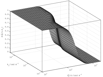
b)

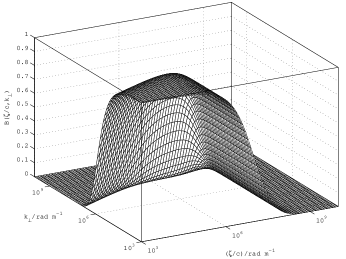
c)

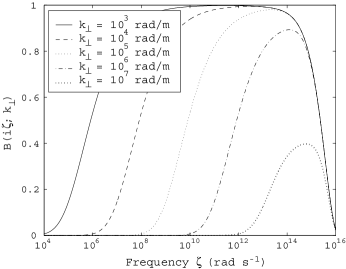
Figure 1: Squared reflection coefficients $A$ and $B$ of the metal interfaces as defined in (7) for the TM and TE modes, as a function of $\zeta/c$ and the transverse momentum $k_{\perp}$. a) $A$ for the TM mode, b) $B$ for the TE mode, c) $B$ for $k_{\perp}$ and $\zeta$ close to zero.

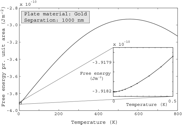
Figure 2: Numerical evaluation of the free energy (6) between two gold halfspaces as a function of temperature. The inset gives details for low $T$.

The vanishing of the zero frequency mode is intimately connected with the behavior of the reflection coefficient $B$ at vanishing frequency. According to the Drude model (or any model satisfying (3)) the TE mode reflection coefficient tends to zero as $\zeta\to 0$. To illuminate this point, we have plotted $A$ and $B$ as a function of imaginary frequency and transverse momentum, $k_{\perp}$, for an interface between gold and vacuum in Fig. 1. In part c) of this figure, we clearly see how $B$ vanishes smoothly when $\zeta\rightarrow 0$ for $k_{\perp}\neq 0$ consistent with Maxwell’s equations of electrodynamics. However, the coefficient $A$ in Fig. 1a) for the TM mode equals 1 for all $k_{\perp}$ as $\zeta\rightarrow 0$, as is also the case for for all $\zeta$ for an ideal metal. In the latter limit we also have $B\rightarrow 1$, but for $\zeta=0$, $B$ remains zero.

For ideal or non-ideal metals it is well known that the temperature correction for the TM mode behaves as $T^{4}$. Thus it does not add to the $T^{2}$ and $T^{5/2}$ terms that we find from the TE mode .

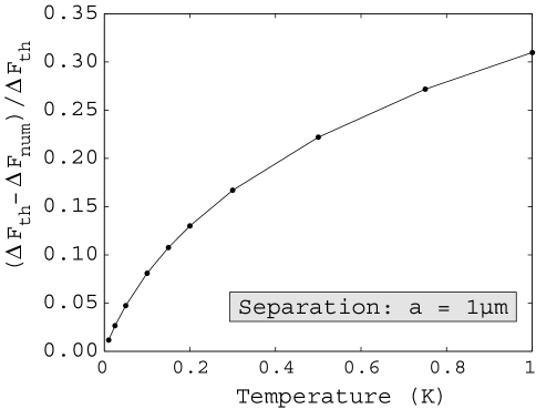
Figure 3: Plot of the ratio $R$ defined in Eq. (33).

By direct numerical integration and lengthy summations independent of the analytic derivations made in Section 2, we obtain the free energy numerically. Figure 2 shows the free energy versus temperature up to 800 K, while the inset shows details of the parabolic shape close to $T=0$. First of all the figure shows the controversial decrease of the magnitude of the Casimir free energy and thus also the related decrease of the Casimir force up to a certain temperature. Secondly, the inset shows that the tangent of the curve is horizontal at $T=0$ as predicted. This implies that the entropy due to the Casimir force is indeed zero at $T=0$. Thus the Nernst theorem is not violated when using the realistic Drude dispersion model. In contrast, it would be violated if a TE-term were added for $\zeta=0$. This conclusion, as mentioned above, is clearly in contrast to that presented in various earlier works [18, 19, 20, 21, 22]. The reader should note that the dependency of $\nu$ on temperature has been neglected in figure 2.

Now there are always some uncertainties connected with numerical calculations. Also the analytic derivation has some uncertainties , e.g., concerning proper use of the Euler-Maclaurin formula, and concerning convergence and neglect of of higher order terms. In Fig.3 we have therefore made a more accurate and much more sensitive test of the behavior near $T=0$ comparing the analytic result with the numerical one, by plotting the ratio $R$ defined in Eq. (33). We see that $R$ when extrapolated approaches zero linearly with a finite slope (when taking the curvature of the plot into account). Thus, with high accuracy we find full agreement concerning the $T^{2}$ and $T^{5/2}$ terms in the free energy and their coefficients $C_{1}$ and $C_{2}$. As the number of terms to be summed numerically increases rapidly when $T=0$ is approached, our evaluations were terminated at $T=0.008~{}$K. The extrapolated value $R=0$ for $T=0$ means that the coefficient $C_{1}$ is correct while the finite slope means that $C_{2}$ is correct too within numerical uncertainties. Also if a more dominant power were present, $R$ would diverge at $T=0$. The finite slope of $R$ at $T=0$ means that the next term in $\Delta F^{TE}$ is of higher order (see also Appendix B for details).

Acknowledgment

We thank Astrid Lambrecht for providing accurate dispersive data for gold, and we thank Kimball A. Milton for valuable comments.

Appendix A Alternative derivation by expansion of $g(m)$

As a variant of the analytic approach, let us show how the essential dependence of the free energy $F^{TE}$ on $T$ near $T=0$ also can be recovered by making use of complex integration. We begin with the TE expression

$$\beta F^{TE}=C{\sum_{m=0}^{\infty}}^{\prime}m\int_{x_{0}}^{\infty}x\ln(1-Be^{-\alpha x})dx,$$ (A1)

where

$$C=\frac{\omega_{p}^{2}}{\beta\hbar\nu c^{2}},\quad\alpha=2a\sqrt{2\pi Cm}.$$ (A2)

The essential step now is to expand the logarithm to the first term,

$$\beta F^{TE}=-C\sum_{m=1}^{\infty}m\int_{0}^{\infty}xBe^{-\alpha x}dx,$$ (A3)

($m=0$ does not contribute to the sum (A1)), where we have also replaced the lower limit $x_{0}$ by zero. We next use the formula [34]

$$e^{-\alpha x}=\frac{1}{2\pi i}\int_{c-i\infty}^{c+i\infty}ds(\alpha x)^{-s}\Gamma(s),\quad c>0,$$ (A4)

where $\Gamma(s)$ is the gamma function. The summation over $m$ is easily done,

$$\sum_{m=1}^{\infty}m^{1-s/2}=\zeta(\frac{s}{2}-1).$$ (A5)

Here $\zeta$ is the Riemann zeta function, defined by the analytic continuation of

$$\zeta(s)=\frac{1}{\Gamma(s)}\int_{0}^{\infty}\frac{t^{s-1}}{e^{t}-1}dt$$ (A6)

for Re$(s)<1$ [33]. As is known, $\zeta(s)$ is one-valued everywhere except for $s=1$, where it has a single pole with residue 1. As $\Gamma(s)$ has simple poles at $s=-n$ with residue $(-1)^{n}/n!$, $n=0,1,2,...$ we get, by taking $c>4$ and closing the contour of integral (A4) as a large semicircle on the left,

$$\beta F^{TE}=-C\int_{0}^{\infty}Bx\left[\frac{\Gamma(4)}{(2ax)^{4}}\frac{1}{(2\pi C)^{2}}+\zeta(-1)-2ax\sqrt{2\pi C}\,\zeta(-\frac{3}{2})+...\right]dx.$$ (A7)

The first term in (A7) diverges, the reason being that we have replaced the lower limit $x_{0}$ by zero. This term is independent of $T$, and can thus be omitted in the present context. Thus using $\zeta(-1)=-1/12,$ $\zeta(-3/2)=-0.025485$, together with the integrals $\int_{0}^{\infty}Bxdx=1/12$ and $\int_{0}^{\infty}Bx^{2}dx=8/105$ gives the temperature-dependent free energy to first order in $B$.

However, this is easily extended to arbitrary order in $B$ by expansion of the integrand in (A1) since $(B\,e^{-\alpha x})^{n}=B^{n}(1-\alpha nx+\frac{1}{2}(\alpha nx)^{2}+\cdots)$. Thus by summation $xB\rightarrow x\sum_{n=1}^{\infty}B^{n}/n=-x\ln(1-B)$ and $x(Bx)\rightarrow x\sum_{n=1}^{\infty}(nB^{n}/n)x=x^{2}B/(1-B)$. By this the above integrals become those of Eqs. (15) and (29), and for the temperature dependent part of the free energy we thus get

$$\Delta F^{TE}=-\frac{C}{\beta}\left[-g^{\prime}(0)\,\zeta(-1)-2a\sqrt{2\pi C}I\,\zeta\left(-\frac{3}{2}\right)+\cdots\right]$$

$$=\frac{C}{\beta}\left[-\frac{1}{12}g^{\prime}(0)\right]\left[1-8\,\zeta\left(-\frac{3}{2}\right)\frac{3a\sqrt{2\pi C}}{-12g^{\prime}(0)}+\cdots\right].$$ (A8)

fully consistent with result (30). Note that $\zeta(-3/2)$ is close to the approximate value (24) and even closer to the more accurate value (25). Thus we have reason to consider $\zeta(-3/2)$ to be the exact result for the Euler-Maclaurin expansion performed in Sec. 2.

Appendix B Remarks on the quantity $R$

Let us explain in some more detail the interpretation of the quantity $R$, defined in Eq. (33). This quantity gives the relative difference between the temperature dependent theoretical free energy $\Delta F_{th}^{TE}$, having the form (32), and the temperature dependent numerical free energy $\Delta F_{num}^{TE}$ calculated from Eq. (6). (As mentioned in Sec. 3, the TM mode behaves as $T^{4}$ and is thus negligible near $T=0$.)

Let us assume that $\Delta F_{th}^{TE}$ has the same form (32) as before, with coefficients $C_{1}$ and $C_{2}$, and that $\Delta F_{num}^{TE}$ has the form

$$\Delta F_{num}^{TE}=D_{1}(T^{2}-D_{2}T^{5/2}+D_{3}T^{3}+\cdots),$$ (B1)

with calculated values for the coefficients $D_{1}$, $D_{2}$, and $D_{3}$. Then,

$$R=\frac{\Delta F_{th}^{TE}-\Delta F_{num}^{TE}}{\Delta F_{th}^{TE}}=\frac{C_{1}-D_{1}}{C_{1}}+\frac{D_{1}}{C_{1}}(D_{2}-C_{2})T^{1/2}+\frac{D_{1}}{C_{1}}(C_{2}D_{2}-D_{3})T+\cdots$$ (B2)

If $C_{1}=D_{1}$ and $C_{2}=D_{2}$, we see that $R$ is zero at $T=0$ and is linear in $T$ for low $T$. From Fig. 3 we see that the fit is perfect insofar as it may be determined from the graph. A constant term would have caused a nonzero value at $T=0$, and a nonzero $T^{1/2}$ term would have caused a vertical slope near $T=0$. None of these effects are perceivable within the numerical accuracy, from which we must conclude that $C_{1}$ and $C_{2}$ are correct within numerical accuracy.

References

- [1] J. S. Høye, I. Brevik, J. B. Aarseth, and K. A. Milton, Phys. Rev. E 67, 056116 (2003).
- [2] I. Pirozhenko, A. Lambrecht and V. B. Svetovoy, New. J. Phys. 8 238 (2006)
- [3] A. Lambrecht and S. Reynaud, Eur. Phys. J. D 8, 309 (2000).
- [4] A. Lambrecht and S. Reynaud, Phys. Rev. Lett. 84, 5672 (2000).
- [5] I. Brevik and J. B. Aarseth, J. Phys. A: Math. Gen. 39, 6187 (2006).
- [6] Handbook of Physics, edited by E. U. Condon and H. Odishaw, 2nd ed. (McGraw-Hill), New York, 1967),Eq. (6.12).
- [7] Khoshenevisan, W. P. Pratt, Jr., P. A. Schroeder, and S. D. Steenwyk, Phys. Rev. B 19, 3873 (1979).
- [8] I. Brevik, J. B. Aarseth, J. S. Høye, and K. A. Milton, in Quantum Field Theory under the Influence of External Conditions, edited by K. A. Milton (Rinton Press, Princeton, NJ, 2004), p. 54.
- [9] I. Brevik, J. B. Aarseth, J. S. Høye, and K. A. Milton, Phys. Rev. E 71, 056101 (2005).
- [10] J. S. Høye, I. Brevik, J. B. Aarseth, and K. A. Milton, J. Phys. A: Math. Gen. 39, 6031 (2006).
- [11] I. Brevik, S. A. Ellingsen, and K. A. Milton, New J. Phys. 8, 236 (2006).
- [12] S. A. Ellingsen, J. Phys. A: Math. Theor. 40, 1951 (2007).
- [13] S. A. Ellingsen and I. Brevik, J. Phys. A: Math. Theor.40, 3643 (2007).
- [14] B. Jancovici and L. Šamaj, Europhys. Lett. 72, 35 (2005).
- [15] P. R. Buenzli and Ph. A. Martin, Europhys. Lett. 72, 42 (2005).
- [16] M. Boström and Bo E. Sernelius, Phys. Rev. Lett. 84, 4757 (2000).
- [17] Bo E. Sernelius, J. Phys. A: Math. Gen. 39, 6741 (2006).
- [18] V. B. Bezerra, G. L. Klimchitskaya, V. M. Mostepanenko, and C. Romero, Phys. Rev. A 69, 022119 (2004).
- [19] R. S. Decca, D. López, E. Fischbach, G. L. Klimchitskaya, D. E. Krause, and V. M. Mostepanenko, Ann. Phys. (NY) 318, 37 (2005).
- [20] V. B. Bezerra, R. S. Decca, E. Fischbach, B. Geyer, G. L. Klimchitskaya, D. E. Krause, D. López, V. M. Mostepanenko, and C. Romero, Phys. Rev. E 73, 028101 (2006).
- [21] V. M. Mostepanenko, V. B. Bezerra, R. Decca, B. Geyer, E. Fischbach, G. L. Klimchitskaya, D. E. Krause, D. López, and C. Romeo, J. Phys. A: Math. Gen. 39, 6589 (2006).
- [22] V. M. Mostepanenko, e-print quant-ph/0702061; G. L. Klimchitskaya, U. Mohideen, and V. M. Mostepanenko, J. Phys. A: Math. Theor. 40, F339 (2007).
- [23] K. A. Milton, The Casimir Effect: Physical Manifestation of Zero-Point Energy (World Scientific, Singapore, 2001).
- [24] M. Bordag, U. Mohideen, and V. M. Mostepanenko, Phys. Rept. 353, 1 (2001).
- [25] K. A. Milton, J. Phys. A: Math. Gen. 37, R209 (2004).
- [26] V. V. Nesterenko, G. Lambiase, and G. Scarpetta, Riv. Nuovo Cimento 27 No. 6, 1 (2004).
- [27] S. K. Lamoreaux, Rep. Prog. Phys. 68, 201 (2005).
- [28] J. Phys. A: Math. Gen. 39 No. 21 (2006) [Special issue: Papers presented at the 7th Workshop on Quantum Field Theory under the Influence of External Conditions (QFEXT05), Barcelona, Spain, September 5-9, 2005].
- [29] New J. Phys. 8 No. 236 (2006) [ Focus issue on Casimir Forces].
- [30] J. M. Obrecht, R. J. Wild, M. Antezza, L. P. Pitaevskii, S. Stringari, and E. A. Cornell, Phys. Rev. Lett. 98, 063201 (2007).
- [31] B. Geyer, G. L. Klimchitskaya, and V. M. Mostepanenko, Phys. Rev. D 72, 085009 (2005).
- [32] G. L. Klimchitskaya, B. Geyer, and V. M. Mostepanenko, J. Phys. A: Math. Gen. 39, 6495 (2006).
- [33] E. Elizalde, S. D. Odintsov, A. Romeo, A. A. Bytsenko, and S. Zerbini, Zeta Regularization Techniques with Aplications (World Scientific, Singapore, 1994).
- [34] E. T. Whittaker and G. N. Watson A Course of Modern Analysis (Cambridge University Press, 1962) p. 280.