Immeasurability of Zero-point Energy in the Cosmological Constant problem

Abstract

A huge discrepancy between the zero-point energy calculated from quantum theory and the observed quantity in the Universe has been one of the most illusive problems in physics. In order to examine the measurability of zero-point energy, we construct reference frames in a given measurement using observables. Careful and explicit construction of the reference frames surprisingly reveals that not only is the harmonic oscillator fluctuating at the ground level, but so is the reference frame when the measurement is realized. The argument is then extended to examine the measurability of vacuum energy for a quantized electromagnetic field, and it is shown that while zero-point energy calculated from quantum theory diverges to infinity, it is not measurable.

Vacuum, unlike its common perception as emptiness, plays an important role in modern physics. With the development of quantum mechanics, it was soon discovered that, due to the uncertainty principle, the vacuum in quantum theory is not empty, but exists at a non-zero level of energy. This observation presents a significant problem, known as the cosmological constant problem, due to the huge discrepancy between the calculation of vacuum energy from quantum theory and the measured quantity from the direct observation in the Universe (see peebles ; straumann and the references therein).

Let us provide a simple example which will give an outline of the main argument to be presented in this paper. For a particle in one-dimensional classical harmonic oscillation, its position is described as a function of time as follows $x(t)=\eta_{1}\cos(\omega t+\phi)$. Let us now suppose there is a detector positioned on another harmonic oscillator that is also oscillating with the same phase and with the amplitude $\eta_{2}$ as follows, $y(t)=\eta_{2}\cos(\omega t+\phi)$. If we assume $\eta_{1}$ and $\eta_{2}$ are non-negative and $\eta_{2}\leq\eta_{1}$, then the detector would measure the position of the particle as follows, $x(t)-y(t)=(\eta_{1}-\eta_{2})\cos(\omega t+\phi)$ and would observe the energy to be $\frac{1}{2}m\omega^{2}(\eta_{1}-\eta_{2})^{2}$. Note that if $\eta_{1}$ is non-zero, then the energy of the particle oscillation is also non-zero. However, this value does not fully contribute to the measured quantity but only the difference contributes to the observed energy. Also note that when $\eta_{2}=\eta_{1}$, the observed energy is zero.

Therefore, even when the energy of the particle is not zero, if the detector is also oscillating as discussed above, the energy may not be measurable by the detector. In this paper, we will present a similar case for zero-point energy of quantum fields. In quantum theory, observables are referred to as a quantity that can be measured, such as position, momentum or a spin. We will construct reference frames from observables and this will provide us with a tool to examine the measurability of zero-point energy. Interestingly, it will turn out that both the constructed reference frames and the state vectors being measured could be in one of the same possible states. Remarkably, this shows that not only is the harmonic oscillator fluctuating at the ground level, but so is the reference frame when the measurement is done. Since a quantum field may be considered as an infinite collection of harmonic oscillators, this argument naturally generalizes to the case of a quantum field. It will be shown that while each harmonic oscillator has non-zero energy at the ground level, the reference frame for each harmonic oscillator could also be sitting only at the same non-zero energy level, thereby, the measurement outcome only yields zero.

Let us begin by examining measurability in the case of a single qubit. A qubit, a basic unit of quantum information nielsen , is a two-level quantum system written as $|\psi\rangle=a|0\rangle+b|1\rangle$ where $a,b$ are complex numbers. Since our goal is to construct a measurement reference frame and a qubit is defined in two-dimensional complex vector space, it would be convenient to consider the qubit as an object that is easier to be visualized, i.e., as a unit vector in the Bloch sphere notation. Using a Bloch sphere notation, i.e., with $a=\exp(-i\phi/2)\cos(\theta/2)$ and $b=\exp(i\phi/2)\sin(\theta/2)$, a qubit in a density matrix form can be written as $|\psi\rangle\langle\psi|=\frac{1}{2}({\bf{1}}+\hat{\nu}\cdot\vec{\sigma})$ where $({{\hat{\nu}}}_{x},{{\hat{\nu}}}_{y},{{\hat{\nu}}}_{z})$ $=(\sin\theta\cos\phi,\sin\theta\sin\phi,\cos\theta)$ and $\vec{\sigma}=(\sigma_{x},\sigma_{y},\sigma_{z})$ where $\sigma_{x}=|0\rangle\langle 1|+|1\rangle\langle 0|$, $\sigma_{y}=-i|0\rangle\langle 1|+i|1\rangle\langle 0|$, and $\sigma_{z}=|0\rangle\langle 0|-|1\rangle\langle 1|$. Therefore a qubit, $|\psi\rangle\langle\psi|$, can be represented as a unit vector ${{\hat{\nu}}}=({{\hat{\nu}}}_{x},{{\hat{\nu}}}_{y},{{\hat{\nu}}}_{z})$ pointing in $(\theta,\phi)$ of a sphere with $0\leq\theta\leq\pi,0\leq\phi\leq 2\pi$. Having the notation of writing the qubit in a sphere, we wish to construct a reference frame in measuring the qubit in the same sphere. In particular, we wish to use observables in quantum theory. Similar to the case of a qubit, an observable can also be written as a unit vector in the Bloch sphere, ${{\hat{\nu}^{\prime}}}=({{\hat{\nu}^{\prime}}}_{x},{{\hat{\nu}^{\prime}}}_{y},{{\hat{\nu}^{\prime}}}_{z})$ where $({{\hat{\nu}^{\prime}}}_{x},{{\hat{\nu}^{\prime}}}_{y},{{\hat{\nu}^{\prime}}}_{z})$ $=(\sin\vartheta\cos\varphi,\sin\vartheta\sin\varphi,\cos\vartheta)$, pointing $(\vartheta,\varphi)$ direction in a sphere. Therefore if one is to make a measurement in $(\vartheta,\varphi)$ direction, the observable would be ${{\hat{\nu}^{\prime}}}\cdot\vec{\sigma}$.

Note that using the introduced notation, both the state vector and observables are written as unit vectors in the Bloch sphere. If we consider the qubit to be a spin-1/2 particle pointing in some direction $(\theta,\phi)$, the spin could be either pointing up or down in that particular direction. It was noted that just as the state vector can be either spin-up or spin-down in a given direction, $(\theta,\phi)$ in the Bloch sphere, so is the reference frame, i.e., the vector representing the observable can be either up or down in a given direction. For simplicity, let us choose the spin-1/2 particle to be pointing in $z$-direction. As pointed out, the particle could be either pointing in $+z$-direction ($\hat{\nu}=(0,0,1)$) or $-z$-direction ($\hat{\nu}=(0,0,-1)$). If this particle is to be measured in $z$-direction, there are two choices of reference frame, i.e., $+z$-direction ($\hat{\nu}^{\prime}=(0,0,1)$) or $-z$-direction ($\hat{\nu}^{\prime}=(0,0,-1)$). Suppose the particle is initially prepared in spin-up $z$-direction. If the particle is measured with an observable pointing up in $z$-direction, the eigenvalue outcome would be $+1$. This then implies that the particle’s spin is in the same direction as the measurement reference frame, $z$, and it could be concluded that the spin is pointing up in $z$ direction. However, if the measurement reference frame is chosen as pointing down in $z$-direction, $\hat{\nu}^{\prime}=(0,0,-1)$, then the eigenvalue outcome would be $-1$. Obtaining $-1$ implies that the particle’s spin is in the opposite direction as the measurement reference frame, i.e., $-z$ in this case, and therefore, it could be concluded that the particle’s spin is pointing in $+z$. Notice that the reference frame for measurement is not outside of spin up or down in $z$-direction and the measurement result yields spin up or down. The reference frame also lies either up or down just as the particle does. The measurement outcome only tells us if the spin is in the same direction ($+1$) or in the opposite direction ($-1$) as the reference frame, instead of up or down. This observation, where the reference frame not being outside of spin up or down, will be important in considering the reference frame for energy eigenvectors for harmonic oscillators. Moreover, for identically prepared states, the measurement outcomes are opposite depending on the choice of reference frames. That is, the eigenvalue outcomes $\pm 1$ are not the absolute values but they depend on the reference frame of a given measurement. This point will be relevant when we consider the case of harmonic oscillator that the only the relevant quantity of energy eigenvalues will be measurable.

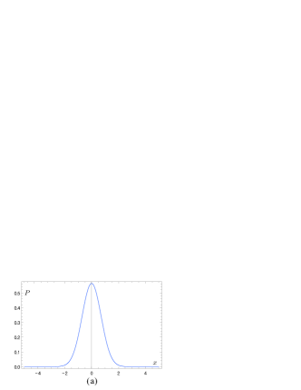
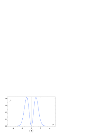
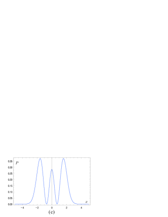
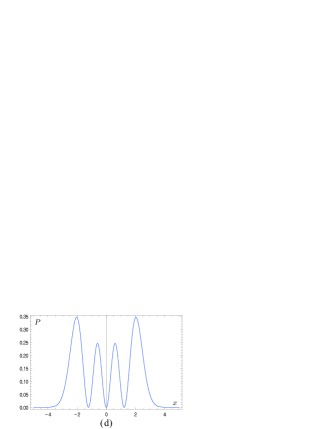
Figure 1: First four probability distribution of energy state of a harmonic oscillator in the position space where we have set $\hbar/m\omega=1$.

Since a quantum field can be considered as an infinite collection of harmonic oscillators, we wish to present our argument starting with a single harmonic oscillator (see sakurai for a review). A Hamiltonian for a single one-dimensional quantum harmonic oscillator is written in terms of position and momentum operators as follows, $\hat{H}=\hat{p}^{2}/2m+m\omega^{2}\hat{x}^{2}/2$. With the introduction of raising and lowering operators, $a^{\dagger}=1/\sqrt{2}(\sqrt{m\omega/\hbar}\hat{x}-i\sqrt{1/m\hbar\omega}\hat{p})$ and $a=1/\sqrt{2}(\sqrt{m\omega/\hbar}\hat{x}-i\sqrt{1/m\hbar\omega}\hat{p})$, the Hamiltonian can be re-written as $\hat{H}=\hbar\omega(N+1/2)$ where $N$ is a number operator, $N=a^{\dagger}a$. The eigenvectors of Hamiltonian can be obtained from the following relations, $\hat{H}|\varepsilon_{n}\rangle=\varepsilon_{n}|\varepsilon_{n}\rangle$ where $\varepsilon_{n}=(n+\frac{1}{2})\hbar\omega$. Let us write the Hamiltonian, or the energy observable, in terms of its eigenvectors as follows, $\hat{H}=\varepsilon_{n}|\varepsilon_{n}\rangle\langle\varepsilon_{n}|$. In order to consider a measurement of the energy eigenstate, we wish to consider the measurement in the position space. In order to measure an energy state $|\varepsilon_{n}\rangle$ in the position space, the outcome can be calculated as $|\varepsilon_{n}\rangle=\int_{x}|x\rangle\langle x|\varepsilon_{n}\rangle$. Therefore, for a given state $|\varepsilon_{n}\rangle$, the measurement outcome would yield the state $|x\rangle$ with the probability, $|\langle x|\varepsilon_{n}\rangle|^{2}$, as follows

$$\frac{1}{2^{n}\sqrt{\pi}n!}\left(\frac{\hbar}{m\omega}\right)^{n-\frac{1}{2}}\left|\left(\frac{m\omega}{\hbar}x-\frac{d}{dx}\right)^{n}e^{\frac{-m\omega}{2\hbar}x^{2}}\right|^{2}$$ (1)

The first four probability distributions are shown in Fig. 1. When the energy state is measured in the position space, and the probability distribution is obtained as in (a) of Fig. 1, then one can determine the energy is in the ground state $|\varepsilon_{0}\rangle$. If the position distribution comes out as seen in (b) of Fig. 1, then it can be determined that the energy state corresponds to $|\varepsilon_{1}\rangle$. Similarly, for (c) and (d), they correspond to $|\varepsilon_{2}\rangle$ and $|\varepsilon_{3}\rangle$, respectively, etc. Our goal was to construct reference frames in measuring the energy state analogous to the qubit case. In order to do so, let us consider the following commuting energy observables defined as follows, $\sum_{m=0}^{\infty}\varepsilon_{m}|\varepsilon_{m+\ell}\rangle\langle\varepsilon_{m+\ell}|$ where $\ell=0,1,2,...$. One can see that, when $\ell=0$, it is identical to the Hamiltonian we studied above. Let us consider the case when $\ell=1$. In such case, when the energy state is $|\varepsilon_{m}\rangle$, the eigenvalue obtained after a measurement would correspond to $\varepsilon_{m-1}$. As was discussed above, we may consider the measurement in the position space. Therefore, when the probability distribution is obtained as in (a) of Fig. 1, then the energy state corresponds to $|\varepsilon_{1}\rangle$. Similarly, when the probability distribution is obtained as in (b), then $|\varepsilon_{2}\rangle$ is the energy state and so on. Similarly, for higher values of $\ell$ for the commuting energy observables, measurements in the position space would yield the determination of the corresponding energy states.

While we have provided energy states and observables, it is not immediately clear how the commuting observables as defined above provide reference frames in measuring the energy states. Although measurement of a energy state $|\varepsilon_{n}\rangle$ in the position space yields the probability shown in (1) (also see Fig. 1), the average value of $x_{n}$ which corresponds to $\varepsilon_{n}=(n+1/2)\hbar\omega$ can be obtained. In fact, the average of $x_{n}$ is zero as can be seen in Fig. 1, however, the expectation value of ${\hat{x}}^{2}$ yields an appropriate value for the energy eigenvalue i.e., $\langle\varepsilon_{n}|{\hat{x}}^{2}|\varepsilon_{n}\rangle=(2n+1)\hbar/2m\omega$. Since the indication of the position state, along with the momentum, could represent the energy state, we wish to introduce the notation of a position vector $\vec{\lambda}_{n}$ to represent $(2n+1)\hbar/m\omega$. It can be checked that the separation between two adjacent vectors $\vec{\lambda}_{j}$ and $\vec{\lambda}_{j+1}$ is $\Delta\lambda=2\hbar/m\omega$ which leads to the energy difference $\hbar\omega$ between two adjacent levels. Therefore, the energy state can now be viewed as a particle being at one of the equally spaced positions in a one-dimensional coordinate starting at $\vec{\lambda}_{0}=\hbar/m\omega$.

Let us construct reference frames in terms of the newly defined position vectors from energy observables, $\sum_{m=0}^{\infty}\varepsilon_{m}|\varepsilon_{m+\ell}\rangle\langle\varepsilon_{m+\ell}|$ where $\ell=0,1,2,...$. In case of a qubit, we constructed reference frames from observables such that the reference frames ended up having the same degrees of freedom as the qubit being measured. We also noted that the eigenvalue outcomes depended on the reference frame, i.e., when the outcome was $+1$ ($-1$), this meant the particle’s spin is in the same (opposite) direction as the reference frame. With these two criteria we wish to consider the observables $\sum_{m=0}^{\infty}\varepsilon_{m}|\varepsilon_{m+\ell}\rangle\langle\varepsilon_{m+\ell}|$ as a detector positioned at $(2n+1)\hbar/m\omega$, which we will denote with a position vector $\vec{\lambda}_{n}^{\prime}$ just as in the case of eigenvectors. Let us examine how this particular construction is consistent with the qubit case. Note that just as a particle could be placed on one of the equally spaced $\vec{\lambda}_{i}$’s, so is the detector. This is analogous to the qubit case where just as particle’s spin could be up or down in a given direction, so is the reference frame in measuring the qubit. Suppose the detector is positioned at $\hbar/m\omega$, i.e., its reference frame corresponds to a vector $\vec{\lambda}_{0}^{\prime}$. When the particle is also positioned at $\lambda_{0}$, i.e., at the ground level, then the outcome would yield zero, meaning the particle’s position is the same as the detector, i.e., $\hbar/m\omega$. Notice that while the measurement outcome is zero, the result reveals that the particle is positioned at $\hbar/m\omega$. When the particle is at $\lambda_{1}$ and the detector is positioned at $\lambda_{0}$, then the outcome would be $\Delta\lambda=2\hbar/m\omega$. However, if the detector is positioned at $\lambda_{1}$, i.e., the reference frame of $\vec{\lambda}_{1}^{\prime}$, measuring the same particle positioned at $\lambda_{1}$ would yield zero rather than $2\hbar/m\omega$. Just as in the qubit case, the measurement outcomes are relative, i.e., they depend on where the detector is positioned at. Therefore, representing energy states and observables through the position vectors $\vec{\lambda}_{i}$ and $\vec{\lambda}_{j}^{\prime}$, respectively, leads us to view the states and reference frames in a clearer picture similar to the case of the Bloch sphere with a qubit. That is, it provides us to show why ground state of a harmonic oscillator is non-zero, yet is not measurable.

We now wish to construct reference frames in measurement for quantum fields. In particular, we wish to study the measurability of quantized electromagnetic field in quantum optics (see vedral for a review). Quantizing the electromagnetic field involves considering the Maxwell’s equation in the absence of charges. From classical Maxwell’s equations in a vacuum, one could obtain the following equation,

$$\nabla^{2}A=\frac{1}{c^{2}}\frac{\partial^{2}A}{\partial t^{2}}$$ (2)

The solution to this has the following form, $A=\sum_{k}(u_{k}(t)v_{k}(r)+c.c.)$. With separation of variables, we could obtain the two equations for $u_{k}(t)$ and $v_{k}(r)$, and the solutions to these equations yield the following for the vector potential,

$$A=\sum_{k}\left(b_{k}{\bf{e}}_{k}e^{-i\omega t}e^{ik\cdot r}+c.c.\right)$$ (3)

where ${\bf{e}}_{k}$ is a unit polarization vector and we are assuming the frequency $\omega$ to be the same for all $k$ modes for simplicity. The classical Hamiltonian of the electromagnetic field is written as

$$H=\frac{1}{2}\int dV(\epsilon_{0}E^{2}+\frac{1}{\mu_{0}}B^{2})$$ (4)

where $\epsilon_{0}$ and $\mu_{0}$ are electric permittivity and magnetic permeability, respectively, that are related to the speed of light, $c=1/\sqrt{\epsilon_{0}\mu_{0}}$. Since $B=\nabla\times A$ and $E=-\partial A/\partial t$ and with newly defined variables, $b_{k}=\sqrt{1/4V\epsilon_{0}}(x_{k}+ip_{k}/\omega)$ and $b_{k}^{*}=\sqrt{1/4V\epsilon_{0}}(x_{k}-ip_{k}/\omega)$, we could obtain the Hamiltonian in the following form,

$$H=\frac{1}{2}\sum_{k}(p_{k}^{2}+\omega^{2}x_{k}^{2})$$ (5)

Quantization can be achieved by replacing $x$ and $p$ with operators ${\hat{x}}$ and ${\hat{p}}$ which follow the usual commutation rules. Now with the newly defined operators

$${\hat{a}}_{k} = \sqrt{\frac{1}{2\hbar\omega}}\left(\omega{\hat{x}}_{k}+i{\hat{p}}_{k}\right)$$

$${\hat{a}}_{k}^{\dagger} = \sqrt{\frac{1}{2\hbar\omega}}\left(\omega{\hat{x}}_{k}-i{\hat{p}}_{k}\right)$$ (6)

the Hamiltonian can be re-written as

$$H=\sum_{k}\hbar\omega({\hat{a}}_{k}^{\dagger}{\hat{a}}_{k}+\frac{1}{2})$$ (7)

If we define the number operator as $N_{k}={\hat{a}}_{k}^{\dagger}{\hat{a}}_{k}$, then the Hamiltonian can be written as $H=\sum_{k}\hbar\omega(N_{k}+1/2)$. Therefore, it can be seen that the quantized electromagnetic field can be considered as an infinite collection of decoupled harmonic oscillators with frequency $\omega$ where the decoupled eigenvectors are $|\varepsilon_{n_{1}}\rangle_{1}\otimes|\varepsilon_{n_{2}}\rangle_{2}\otimes\cdots$. The energy of ground state, a zero-point energy, can be calculated as

$${\mathcal{E}}=\sum\varepsilon_{0,m}=\sum_{m=1}^{\infty}\frac{1}{2}\hbar\omega$$ (8)

where $\varepsilon_{j,m}$ is the eigenvalue for $m$th mode eigenvector $|\varepsilon_{j}\rangle_{m}$ and it can be seen that this value diverges to infinity. In quantum optics vedral , measurement of eigenvectors is done with photon number counting of $N_{k}$ for each mode $k$. Therefore for a $k$th detector, when the photon numbers are registered as $n_{k}$, then the energy state corresponds to $|\varepsilon_{n_{k}}\rangle_{k}$.

In the cases of a qubit and a single harmonic oscillator, we introduced commuting observables in order to construct reference frame in a similar way to state vectors. For a quantum field we wish to do the same and introduce commuting observables as follows, $\sum_{m}\varepsilon_{m,1}|\varepsilon_{m+\ell_{1}}\rangle_{11}\langle\varepsilon_{m+\ell_{1}}|\otimes\sum_{m}\varepsilon_{m,2}|\varepsilon_{m+\ell_{2}}\rangle_{22}\langle\varepsilon_{m+\ell_{2}}|\otimes\cdots$. When $\ell_{1}=0,\ell_{2}=0,...$, then the observable is the same as the Hamiltonian described above. In order to realize this observable, i.e., where all $\ell_{k}$’s are zero, when the $k$th photon number is detected as $n_{k}$, then the corresponding energy state would be determined as $|\varepsilon_{n_{k}}\rangle_{k}$. Let us now consider the case when $\ell_{1}=1,\ell_{2}=0,\ell_{3}=0,...$ This observable can be realized by taking $|\varepsilon_{n_{k}}\rangle_{k}$ for the detection of $n_{k}$ photons registered at $k$th detector except, when $k=1$, the $n_{1}$ photon numbers yield $|\varepsilon_{n_{1}+1}\rangle_{1}$. Similarly, when $\ell_{1}=2$ and all other $\ell_{j}$’s are zero, then for $n_{1}$ photon number detection, the state could be determined as $|\varepsilon_{n_{1}+2}\rangle_{1}$, while for $k\neq 1$, the energy states could be decided the same as described above. This analogy can be extended to higher values of $\ell_{1}$ and for other $\ell_{j}$’s. This describes how the commuting observables can be realized with photon number detectors.

In case of a single harmonic oscillator, we used the fact that the average position which corresponds to the appropriate energy state can be useful in constructing reference frames that are easy to visualize. Therefore the energy eigenvectors for a quantum field could be viewed as a collection of particles where each particle is positioned at $\lambda_{j}=(2n_{j}+1)\hbar/m\omega$ on each coordinate. Since we have an infinite number of harmonic oscillators, we rewrite the energy states, $|\varepsilon_{n_{1}}\rangle_{1}\otimes|\varepsilon_{n_{2}}\rangle_{2}\otimes\cdots$, with the following position vectors $\vec{\lambda}_{n_{1},1}\otimes\vec{\lambda}_{n_{2},2}\otimes\cdots$. We now wish to construct reference frames from observables which have the same degrees of freedom as position vectors. For a single harmonic oscillator, we argued that the commuting observables could be pictured as a detector being positioned at $\lambda_{n}=(2n+1)\hbar/m\omega$. In this way, we were able to construct reference frames of measurement. We now wish to extend this to a multiple number of detectors. We will now assume that a detector positioned at $\lambda_{j}=(2j+1)\hbar/m\omega$ on $k$th coordinate to be denoted as $\vec{\lambda}_{j,k}^{\prime}$. This then yields the commuting observables $\sum_{m}\varepsilon_{m,1}|\varepsilon_{m+\ell_{1}}\rangle_{11}\langle\varepsilon_{m+\ell_{1}}|\otimes\sum_{m}\varepsilon_{m,2}|\varepsilon_{m+\ell_{2}}\rangle_{22}\langle\varepsilon_{m+\ell_{2}}|\otimes\cdots$ to be written as $\vec{\lambda}_{\ell_{1},1}^{\prime}\otimes\vec{\lambda}_{\ell_{2},2}^{\prime}\otimes\cdots$ for all modes. Therefore, when all $\ell_{j}$’s are zero, all detectors are positioned at the position of $\hbar/m\omega$ on each coordinate. In the case where $\ell_{0}=1$ while all other $\ell_{j}$’s are zero, the detector for the first mode is positioned at $\lambda_{1}$ while all other detectors are placed on $\lambda_{0}$’s. Similarly, when $\ell_{0}=2$, the 2nd mode detector is placed at $\lambda_{2}$ and so on. When all $\ell_{j}$’s are zero for detectors and $n_{i}$’s are zero for particles, the measurement outcome for each detector would always be zero, implying each particle is in the same position as the corresponding detector, i.e., $\hbar/m\omega$. Suppose the first particle is in the position of $\lambda_{1}$, then the first detector would record the measurement outcome as $\Delta\lambda=2\hbar/m\omega$ while the rest detectors would record zero. However, suppose the second detector is positioned at $\lambda_{2}$, i.e., the observable $\vec{\lambda}_{0,1}^{\prime}\otimes\vec{\lambda}_{2,2}^{\prime}\otimes\vec{\lambda}_{0,3}^{\prime}\otimes\cdots$, and the second particle positioned also at $\lambda_{2}$, i.e., $\vec{\lambda}_{0,1}\otimes\vec{\lambda}_{2,2}\otimes\vec{\lambda}_{0,3}\otimes\cdots$, then all the detectors would still measure only zero. With the construction of reference frames in terms of position $\lambda$’s, it provides a picture that when all particles are at $\lambda_{0}$ and all the detectors are also at $\lambda_{0}$, the measurement outcomes will be zero. Therefore, while the energy of electromagnetic field in vacuum diverges to infinity, the detectors would measure only zero.

We have shown by using the example of a qubit measurement, that the reference frame for the measurement can be constructed using observables in such a way that it could be in one of the same possible states as the qubit could be in. Moreover, the obtained measurement outcomes are shown to be relative with respect to the reference frame. We have applied this analogy to the case of a single quantum harmonic oscillator and argued that just as with the energy eigenvectors, the reference frame for a measurement can only be in the non-zero ground level. This was then extended to the electromagnetic field. It is noted that taking observables as a reference frame for measurement has also yielded an interesting result in regards to the halting problem in quantum computation song .

The author wishes to thank J. Bae for helpful discussions and J.M. Isidro for correspondence on this topic.

References

- (1) P.J. Peebles and B. Ratra, Rev. Mod. Phys. 75, 559 (2003).
- (2) N. Straumann, On the Cosmological Constant problems and the Astronomical Evidence for a Homogeneous Energy Density with Negative Pressure, astro-ph/0203330.
- (3) M.A. Nielsen and I.L. Chuang, Quantum Computation and Quantum Information, Cambridge University press (2000).
- (4) J.J. Sakurai, Modern Quantum Mechanics, Addison-Wesley Publishing Company, Inc. (1985).
- (5) V. Vedral, Modern Foundations of Quantum Optics, World Scientific (2005).
- (6) D. Song, Unsolvability of the halting problem in quantum dynamics, Int. J. Theo. Phys. (in press); quant-ph/0610047.