Abstract

Trapped atomic ions have become one of the most promising architectures for a quantum computer, and current effort is now devoted to the transport of trapped ions through complex segmented ion trap structures in order to scale up to much larger numbers of trapped ion qubits. This paper covers several important issues relevant to ion transport in any type of complex multidimensional rf (Paul) ion trap array. We develop a general theoretical framework for the application of time-dependent electric fields to shuttle laser-cooled ions along any desired trajectory, and describe a method for determining the effect of arbitrary shuttling schedules on the quantum state of trapped ion motion. In addition to the general case of linear shuttling over short distances, we introduce issues particular to the shuttling through multidimensional junctions, which are required for the arbitrary control of the positions of large arrays of trapped ions. This includes the transport of ions around a corner, through a cross or T junction, and the swapping of positions of multiple ions in a laser-cooled crystal. Where possible, we make connections to recent experimental results in a multidimensional T junction trap, where arbitrary 2-dimensional transport was realized.

1 Introduction

Trapped ion systems serve as a promising direction toward realizing an operational quantum computer [1]-[26]. Many experiments in ion trap systems have been performed to show entanglement [4]-[11], fundamental logic gates [11]-[17], and teleportation [18, 19]. Algorithms have even been performed on a small number of trapped ions [20]-[24]. One of the remaining challenges toward realizing a useful quantum information processor is that of scaling up these proof-of-principle experiments.

One proposal for scaling up a trapped ion quantum computer is to create an integrated array of linear rf Paul ion traps, divided into regions for storage and entanglement. Such a device would carry out logical operations by generating two-particle entanglement between any pair of ions by shuttling the ions out from storage into the entanglement zones, and bringing them back into storage as required for the completion of the algorithm [3, 25]. This quantum computing architecture requires arbitrary two-dimensional control of trapped ions that may consist of four key protocols: linear shuttling, corner shuttling, separation and recombination. These key protocols may be combined to produce other necessary operations such as a swapping protocol to switch the positions of two trapped ions [26].

The process of shuttling ions from a storage region to an entanglement region and back requires sophisticated, accurate and detailed knowledge of the time-dependent electric fields in order to control the ions’ dynamics in the trap arrays. For trap arrays containing many ions, the cost of calculating the necessary electric fields for each intermediate set of voltages during a shuttling operation is prohibitive. An alternative approach is to develop a set of numerically-obtained “basis functions,” that represent the contribution to the electric potential seen by the ion due to a unit voltage applied to each of the dc electrodes in the trap array, the others being held at zero voltage. The electric potential produced by an arbitrary set of voltages on the electrodes is calculated by multiplying the basis function for each electrode with the actual applied voltage, and then adding up the corresponding potentials at all points in space.

In order to shuttle ions in an array of linear ion traps, the control voltages are varied in time and the basis function technique is used to calculate the potential as a function of time. To choose the appropriate methods to simulate the ions’ motion in the trap, it is important to determine the purpose of the simulation to be carried out. Typically we will be interested in moving ions between points inside the array successfully while minimizing the kinetic energy that the ion acquires during the shuttling process. This can be simulated by solving the classical equations of motion using the calculated potential. The question arises whether there are important corrections if one considers the full quantum evolution of the system. Berman and Zaslavsky [27] showed that the breakdown of quantum-classical correspondence occurs on a time scale at which the quantum wave function spreads sufficiently over a macroscopic part of phase space to feel anharmonicities in the potential. This is because the quantum evolution of the Wigner function may be expressed as the sum of the Poisson bracket (describing classical evolution) and quantum correction terms that contain higher order spatial potential derivatives [28]. These quantum corrections will be negligible if the ion is shuttled adiabatically (or such that it remains in the Lamb Dicke regime) as the ion remains close to the bottom of the well and the potential may be approximated well as a harmonic potential. Quantum corrections may become important if the ion samples anharmonic parts of the potential. In that case we expect quantum corrections to be important if the shuttling process occurs on timescales that are of order $t_{\hbar}=\frac{1}{\lambda}\ln\left(\frac{A}{\hbar}\right)$ where $\lambda$ is the Lyapunov exponent for the dynamic evolution of the system and $A$ is the action of motion [28]. Nevertheless, it may be that corrections in the calculated electric potential due to the finite accuracy of the numerical solver will weigh stronger than the appearance of quantum-classical divergence. We also point out that the quantum bit of a single ion is always encoded in the internal state of the ion, and we may only require the ion to remain inside the Lamb-Dicke regime after the shuttling process in order to allow the execution of further quantum gate operations. Preserving the actual motional quantum state of the ion during the shuttling process is therefore not likely to be a criterion for the development of shuttling protocols that move ions between interaction and entanglement zones. Finally the ion may also be cooled via sympathetic cooling [29]-[33] after the shuttling operation. Indeed such cooling may also accommodate shuttling operations that fail to confine ions within the Lamb-Dicke regime. Therefore the primary function of the simulation is to provide a highly reliable transport protocol of the ion through the complicated potential inside the array.

This paper is organized in the following way. In the next section, we first discuss the derivation of the electric field inside an ion trap. We then consider the numerical calculation of the resultant classical motion of an ion in this field. In section 3, by determining the quantum mechanical state of the ion after shuttling, we derive constraints and figures of merit that may be used to design and characterize shuttling protocols. In section 4, we compare and contrast salient features of various two-dimensional ion trap architectures, paying particular attention to the junction regions. In section 5, using the T-junction ion trap array as a case study, we consider the practical design and implementation of key ion shuttling protocols. This culminates in the swapping of two ions in a linear chain. In section 6, we briefly consider ion transport and storage in a 3 dimensional array and present conclusions in section 7.

2 Simulation of Trapped Ion Dynamics Via Basis Functions

2.1 Justification of the Basis Function Technique

It is possible to simulate the potential in any complex, multi-zone ion trap by developing electric potential basis functions for a given trap geometry. The electric potential for any arbitrary voltage configuration of the trap electrodes can then be built up as a linear combination of the basis functions. The electric potential of any arbitrary charge configuration with Dirichlet boundary conditions can be written as [34]:

$$\Phi({\bf x})=\frac{1}{4\pi\epsilon_{0}}\int_{V}\rho({\bf x}\,^{\prime})G({\bf x},{\bf x},^{\prime})d\,^{3}{\bf x}\,^{\prime}-\frac{1}{4\pi}\oint_{S}\Phi({\bf x}\,^{\prime})\frac{\partial G({\bf x},{\bf x}\,^{\prime})}{\partial n^{\prime}}da^{\prime}$$ (1)

In Eq. 1, the first integral is an integral over the volume interior to the boundary with the appropriate symmetric Green function $G({\bf x},{\bf x}\,^{\prime})$. Inside of an empty ion trap, there is no free charge so $\rho({\bf x}\,^{\prime})=0$ making the first term of Eq. 1 zero. The second integral is an integral over the surface of each electrode $\Phi({\bf x}^{\prime})$ multiplied by the outward normal derivative of the Green function with respect to the surface $n^{\prime}$. It is possible to write the potential that is specified on every trap electrode as a sum of potentials on each individual electrode with all other electrodes held at ground.

$$\Phi({\bf x}^{\prime})=\sum_{i}\Phi_{i}({\bf x}\,^{\prime})$$ (2)

This changes Eq. 1 to

$$\Phi({\bf x})=-\frac{1}{4\pi}\sum_{i}\oint_{S_{i}}\Phi_{i}({\bf x},^{\prime})\frac{\partial G_{i}({\bf x},{\bf x}\,^{\prime})}{\partial n_{i}^{\prime}}da^{\prime}$$ (3)

As can be seen in Eq. 3, the total electric potential $\Phi(\mathbf{x})$ is a sum of the potentials produced by each electrode surface individually when all other electrodes and boundaries are held at zero potential, as is expected from the linear nature of Laplace’s equation. Since the voltage is constant over each electrode surface, we can rewrite Eq. 3 as a sum of the constant voltage $V_{i}$ times the surface integral only for electrode i in the trap.

$$\Phi(\mathbf{x})=\sum_{i}\frac{-V_{i}}{4\pi}\Bigg{(}\oint_{S^{\prime}}\frac{\partial G(\mathbf{x},\mathbf{x}\,^{\prime})}{\partial n^{\prime}}da^{\prime}\Bigg{)}_{i}=\sum_{i}V_{i}\Theta_{i},$$ (4)

where

$$\Theta_{i}=-\frac{1}{4\pi}\oint_{S^{\prime}}\frac{\partial G(\mathbf{x},\mathbf{x}\,^{\prime})}{\partial n^{\prime}}da^{\prime}$$ (5)

is the basis function for the electric potential produced by the $i$-th electrode held at 1 volt, all others held at ground. The basis functions, as solutions of Laplace’s equation, are strictly valid only for static voltage configurations. However, they are perfectly satisfactory for describing the rf potential and switching potentials used in rf Paul traps, because the shortest wavelengths ($\approx 10^{1}$ m) associated with the time-dependent fields at these frequencies ($\approx 10^{6}$ Hz) will be much greater than the corresponding trap dimensions ($>10^{-3}$ m), allowing us to calculate the fields and potentials in the problem quasi-statically. Effectively, we are considering any changes of the potential in the trap region to be uniform throughout, and essentially simultaneous with the change in the voltage on the electrodes. Therefore, we can introduce time dependence in the switching potentials simply by treating the voltages on the electrodes, $V_{i}$, as functions of time.

The basis function $\Theta_{rf}$ obtained in this manner for the rf electrodes can be used to obtain the potential energy resulting from the rf electrodes in the pseudopotential approximation [35]. The formula for the rf pseudopotential is given by

$$\Psi_{rf}(\mathbf{x},t)=\frac{e^{2}V_{rf}^{2}}{4m\Omega_{T}^{2}}|\mathbf{\nabla}\Theta_{rf}(\mathbf{x})|^{2},$$ (6)

where $V_{rf}$ is the amplitude of the rf voltage applied to the electrodes, $m$ is the mass of the trapped ion, $e$ is the charge on the ion, and $\Omega_{T}$ is the rf angular frequency. Therefore, the rf pseudopotential is found by calculating the square of the electric field amplitude corresponding to the electric potential, $\Theta_{rf}.$ Alternatively, if information about the micromotion of the trapped ion is sought, the time-dependent coefficient of $\Theta_{rf}$ would then become

$$V_{rfmicro}=V_{rf}\cos(\Omega_{T}t).$$ (7)

2.2 Numerical Techniques for Developing Basis Functions

The use of basis functions in the calculation of time-dependent potentials in complex ion trap arrays requires an accurate calculation of each basis function. This basis function is given by the potential produced by each electrode when it is held at $1.0$ V while all other surfaces are held at $0.0$ V. Typically, these functions must be obtained using numerical methods. A well-established and accurate method of obtaining electrostatic potentials produced by a realistic arrangement of electrodes is the finite element method (FEM), which is used in many commercially-available software packages for electromagnetic field simulations. This method requires that the entire bounded problem domain be discretized into a mesh, consisting of nodes and elements. The nodes are related to one another by simple (linear or quadratic) functions, and the solver uses an iterative approach such as energy minimization to obtain the potential at each node so that the boundary conditions are still satisfied. The interpolating functions for each element relating nodal solutions are then used to find the solution throughout the entire solution domain.

The Boundary Element Method (BEM) is an alternative numerical analysis method to the FEM. The BEM starts from the integral equation formulation of the relevant differential equation (Laplace’s equation, in this case). Since there are no charges present in the empty ion trap, only the surface integrals are non-zero. This results in a problem formulation, much like that given in equations 1 through 4, for which the potential within the problem domain is defined by the surface values of the potential and the appropriate Green’s function. If the problem domain is unbounded, then the free space Green’s function for Laplace’s equation can be used. For ion traps, the potential on the surface is prescribed by the applied voltage. The fields at the surface are then found by discretizing the surface with nodes and elements and solving the resulting set of linear equations. This is equivalent to finding the charge density over each element on the surface. The solution at an arbitrary point, P, within the problem domain is found by evaluating the integrals describing the contribution to the potential at P from each charge element on the surface.

A major advantage of the BEM in obtaining basis functions for ion trap arrays is the fact that the discretization of the problem is confined to the boundary surfaces, so that the potential and electric field within the problem domain will be continuous functions. A second advantage is the reduction in dimensionality of the problem (i.e., from a volume to a surface) in the BEM. As larger and larger trap arrays are considered, the bounding box volume for a finite element model will grow more rapidly than the corresponding trap surface area. In these cases, the BEM can prove much more efficient in calculating the basis functions for ion trap arrays. Because the BEM is restricted to linear problems for which an analytic form of the free space Green’s function exists, it is not as commonly used in commercially available software. Several non-commercial (including CMISS) and commercial (SIS’s CPO  and IES’s Coulomb 3D  ) codes use the BEM exclusively or in conjunction with the FEM.

Most commercially available software for calculating electrostatic potentials and fields, such as Tosca from Vector Fields   or Maxwell 3D from Ansoft  , uses the FEM because of its nearly universal applicability for solving differential equations in physics. In the particular case of ion traps, the FEM provides several advantages, including the ability to account for non-linear material properties of the trap electrodes, its ability to determine mechanical and thermal effects on the trap electrodes during trap operation, and having a simple means for estimating errors in the simulation. Nevertheless, care must be taken when using it for analyzing ion traps. In particular, hexahedral elements should be used with quadratic interpolating functions. While triangular and tetrahedral elements are preferable for ease of meshing the problem volume, they require a far greater number of nodes to achieve the same accuracy as can be obtained with hexahedral elements, or bricks. This is so because hexahedral elements are more easily lined up along the equipotential lines in the relevant problem domain. In addition, the regular spacing of hexahedral elements helps avoid serious discretization errors when calculating the potential in regions where competing fields largely cancel. When calculating the rf pseudopotential, the field amplitude is important. Linear interpolating functions will give a constant value of the field throughout the element, a value most accurate at the element’s centroid. Quadratic elements give a more accurate picture of the field throughout each element, although they are costly in terms of computational effort.

In general, a finer mesh and quadratic elements help avoid discretization errors, while larger problem domains are needed to avoid undue influence from the bounding box. These competing needs result in a rapidly growing cost in memory requirements and computational time as the trap arrays increase in complexity. Computational costs can be reduced through the use of symmetry and strategic meshing.

A symmetric linear Paul trap array will typically have a plane of symmetry in the plane of the rf electrode layer, and another plane perpendicular to the first along the linear trap axis. The $z-$axis is taken to be directed out of the plane of the two-dimensional trap array, and the trap axis is taken to lie along the $y$-axis. Since in the calculation of $\Theta_{rf}$ all electrodes except the rf-layer are set to ground, the boundary conditions on the electrodes preserve the symmetry of the trap, and it becomes possible to reduce the computational domain volume for the rf fields by using the $yx$ and $xz$ symmetry planes as external boundaries of the problem. If the boundary conditions along these planes are set so that the resulting electric field is tangent to these planes, then the calculated potential in the reduced volume corresponds to the potential resulting from a symmetric arrangement of electrodes and voltages across the symmetry planes.

The calculations of $\Theta_{i}$ for the control electrodes are not so easily reduced, since the requirement that only the single control electrode be set to 1 volt with all other electrodes held at 0 volts breaks the symmetry of the trap. However, it is possible to use solutions for the potential which do preserve the symmetry of the trap to obtain the desired non-symmetric potential by using linear superposition. Consider a three-layer trap with four control electrodes arranged symmetrically about the trap center as illustrated for a linear trap in Fig. 1, where the basis function $\Theta_{i}$ is sought for the lower left electrode.

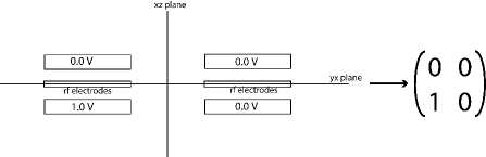
Figure 1: A cross-section view of a 3-layer linear rf ion trap, with four identical dc electrodes placed symmetrically about the two symmetry planes, yx and yz.

We can again reduce the computational volume of the problem by imposing boundaries along the $yx$ and $yz$ symmetry planes. If tangential boundary conditions are applied along both planes, the resulting solution for the potential in the reduced volume corresponds to the case when all four control electrodes in Fig. 1 are held at 1 volt for the full domain. The solution for the full volume is therefore obtained by adding the solution of the reduced volume and appropriate reflections of this reduced volume solution. We identify this solution as

$$tt=\left(\begin{array}[]{cc}+1&+1\\ +1&+1\end{array}\right).$$ (8)

The array identifies the effective voltages on each of the control electrodes when both the symmetry planes have tangential boundary conditions applied. In contrast to tangential boundary conditions, normal boundary conditions on the symmetry planes require that the resulting electric field be normal to the boundary, giving rise to an antisymmetric arrangement of electrodes and an antisymmetric potential. For example, if both symmetry planes had normal boundary conditions, the solution in the reduced problem domain would correspond to the case for the full domain when each neighboring control electrode is of opposite sign, so that

$$nn=\left(\begin{array}[]{cc}-1&+1\\ +1&-1\end{array}\right).$$ (9)

The other two cases involving mixed boundary conditions on the symmetry planes are identified as

$$nt=\left(\begin{array}[]{cc}-1&-1\\ +1&+1\end{array}\right),\hskip 7.22743pt\mbox{and }tn=\left(\begin{array}[]{cc}+1&-1\\ +1&-1\end{array}\right).$$ (10)

As we have shown in Sec. 2, each of these potentials can be decomposed into sums of four potentials corresponding to the contribution from each electrode separately. Each solution, $tt,nn,tn,$ and $nt$, contains a mixture of those contributions. By combining the four solutions in the appropriate manner and dividing by 4, it should therefore be possible to extract the contribution from any one of the single control electrodes. This can be shown symbolically by adding the four solutions, as shown below. The use of the arrays to symbolize the solutions for each symmetry case makes it clear that this process corresponds to adding the boundary conditions on the four electrodes together. The result is a solution for the whole space potential that is produced solely by a unit voltage on the lower left electrode, all other electrodes being held at ground.

$$\frac{tt+nn+tn+nt}{4}=\left(\begin{array}[]{cc}0&0\\ 1&0\end{array}\right)=\Theta_{\mbox{lower left}}$$ (11)

The basis functions for the other three electrodes are easily obtained by the appropriate coordinate reflections of the first solution. This approach, although more time-consuming, is necessary when modeling and meshing the entire problem domain becomes prohibitive due to memory restrictions. It enables the experimenter to mesh the model at a higher density for improved accuracy.

The use of hexahedral elements for meshing an ion trap model places a much greater constraint on node spacing than would be the case if tetrahedral elements are used. In the case of Vector Fields’ Opera suite, this means that node placement must be done manually, and then checked for suitability for hexahedral meshing when placement is complete. In particular, the number of nodes on opposing faces of the model must match, so that the elements are able to completely fill the space in the problem domain. Nevertheless, it is possible to concentrate node placement along the channels through which ions will be expected to be shuttled, and along the electrode surfaces near which the potential is expected to exhibit the greatest variation. There will generally be some wasted node density in regions above and below the trap and along the channels beyond the end electrodes, due to the restrictions on the consistency of the hexahedral elements.

Ion traps are generally constructed from good conductors and dielectrics, which exhibit linear behavior under the voltages typically applied in these traps. In such cases, the accuracy of the electrostatic potentials and fields obtained using the FEM (assuming the model is a correct representation of the physical problem) is primarily a function of the local mesh spacing, and only weakly a function of the overall mesh density in the problem definition. In particular, for a local mesh size h in one dimension (corresponding to the mesh point spacing) and using quadratic elements, the error in the calculated potential scales as ${\cal O}(h^{3}),$ while the error in the fields will scale as ${\cal O}(h^{2})$ [36].

Therefore, a reasonable estimate of the error in the FEM solution can be made by halving the mesh point spacing throughout the model, if memory permits, or otherwise, halving the mesh point spacing in the region requiring greatest accuracy, and running the model again. Percentage changes in the calculated potential and field will then give an estimate of the error in the calculation. Thus, if the field calculation at mesh spacing $h$ gives a result $E$ with unknown error $\Delta E$, and a calculation at mesh spacing $h/2$ gives a different result $E^{\prime}$ with unknown error $\Delta E^{\prime}$ then, we can compare the two unknown errors, since error scales with the square of the mesh spacing, that is,

$$\Delta E^{\prime}=\Delta E/4.$$ (12)

Roughly speaking, we can identify the difference in the two solutions at each point as some function of the uncertainties in each solution. The most conservative assumption would be that the two solutions erred in the same sense from the true value, so that their difference is equal to the difference of the two uncertainties, that is

$$(E-E^{\prime})\geq(\Delta E-\frac{\Delta E}{4})=\frac{3}{4}\Delta E.$$ (13)

Thus, we have a loose upper bound on the error in the original solution,

$$|\Delta E|\leq\frac{4}{3}|E-E^{\prime}|.$$ (14)

Once the models have been meshed and analyzed, it is still necessary to evaluate the potential and/or field at each point of interest in the problem domain. In the interest of carrying out simulations of ion trajectories it is desirable, therefore, to obtain beforehand a grid of potential or field amplitude values covering the problem domain volume corresponding to locations where ion trapping and shuttling will take place. The grid spacing used for the array should be at least as small as the nodal spacing used in the numerical simulation. There will be diminishing returns for using even denser arrays of points, since the potentials between the nodes of the finite element mesh are already calculated using quadratic interpolating functions. Since the potentials are solutions of Laplace’s equation and thus smoothly varying functions of position, it is possible to generate splined, interpolating functions from these data grids at the accuracy of the finite element solution to serve as the basis functions $\Theta_{i}$ for subsequent calculations of the ion dynamics.

2.3 Trapped Ion Dynamics

We now consider the desired potential by suitably superposing the basis functions multiplied by the time varying potential

$$U(\mathbf{x},t)=eV_{rf}\cos(\Omega_{T}t)\Theta_{rf}(\mathbf{x})+e\sum_{i}V_{i}(t)\Theta_{i}(\mathbf{x})$$ (15)

where $e$ is the charge of the ion, $\mathbf{x}$ is the position vector, $\Omega_{T}/2\pi$ and $V_{rf}$ are the applied rf frequency and amplitude, $V_{i}(t)$ is the time varying potential applied on the $i$th control electrode and $\Theta_{i}(x)$ is the basis function of the $i$th electrode. Notice here that the coefficient for all the basis functions have explicit time dependence.

The ion’s motion due to the electric potential $\Phi$ will consist of the low amplitude micro-motion with frequency to the order of $\Omega_{T}$ and the slower but larger amplitude secular motion. Very often, we only need to calculate the secular motion of the ion and ignore the micro-motion. Therefore we may approximate Eq. 15 with a ponderomotive pseudopotential given by [35]:

$$\Psi(\mathbf{x},t)=\frac{e^{2}V_{rf}^{2}}{4m\Omega_{T}^{2}}|\mathbf{\nabla}\Theta_{rf}(\mathbf{x})|^{2}+e\sum_{i}V_{i}(t)\Theta_{i}(\mathbf{x})$$ (16)

Finally, if there are k ions in the trap, the resultant force on each ion $\mathbf{F_{j}}$ is given by

$$\mathbf{F_{j}}(\mathbf{x_{1}},...,\mathbf{x_{k}},t)=\left\{\begin{array}[]{ll}-\mathbf{\nabla}U(\mathbf{x_{j}},t)+\frac{1}{4\pi\epsilon_{0}}\sum_{i\not=j}\frac{e^{2}}{|\mathbf{x_{j}}-\mathbf{x_{i}}|^{3}}(\mathbf{x_{j}}-\mathbf{x_{i}})&\textrm{complete ion motion}\\ -\mathbf{\nabla}\Psi(\mathbf{x_{j}},t)+\frac{1}{4\pi\epsilon_{0}}\sum_{i\not=j}\frac{e^{2}}{|\mathbf{x_{j}}-\mathbf{x_{i}}|^{3}}(\mathbf{x_{j}}-\mathbf{x_{i}})&\textrm{ion secular motion only}\end{array}\right.$$ (17)

Therefore, to calculate the dynamics of $k$ ions in a trap we need to solve the set of $k$ coupled second order ordinary differential equations(ODEs):

$$\mathbf{\ddot{x}_{j}}=\frac{\mathbf{F_{j}}}{m}(\mathbf{x_{1}},...,\mathbf{x_{n}},t)\equiv\mathbf{a_{j}}(\mathbf{x_{1}},...,\mathbf{x_{n}},t)$$ (18)

where $j$ is an integer from 1 to $k$. Determining the classical motion of trapped ions plays an important role in calculating the energy gained during shuttling as will be seen in section 3.

2.4 Numerical Methods for Obtaining Trapped Ion Dynamics

In general, there is no analytic solution for the electric field in an ion trap, so Eq. 18 must be solved numerically. As will be seen in Section 3, the classical motion of trapped ions during shuttling protocols will play an important role in calculating the amount of heating the ions undergo from an arbitrary initial quantum state. The design of shuttling protocols requires high accuracy solutions of Eq. 18 and as such the numerical evaluation of Eq. 18 can be slow. High accuracy solutions are needed to optimize shuttling protocols by minimizing the acquired kinetic energy from shuttling. Using an AMD dual core 1.8GHz processor with 2 GB of memory to calculate the trajectory of the ion with a shuttling sequence that shuttles an ion around a corner of a T-junction ion trap array, the computer time taken to obtain the ion trajectory depends on the ODE solver method ranges from 5 hours to a full week. In complex shuttling operations where hundreds of ions may be shuttled throughout an ion trap array, one must make a judicious choice of ODE solver in order to reach the required accuracy in a feasible amount of time.

Explicit extrapolation class methods are good for efficiently (minimal computing time) solving ODE’s to high accuracy [37]. However, a caveat when using this class of methods is that the calculated electric field has to be smooth. If the electric field is rough, Explicit Runge-Kutta (ERK) methods may be a better choice [38]. In addition, if a low accuracy solution is sufficient, single step methods tend to be more efficient than the extrapolation class methods [38]. This section outlines the reasons why the Bulirsch-Stoer method effectively simulates ion motion in ion trap arrays while Appendix A discusses how the Bulirsch-Stoer (B.-S.) method works.

The ODE system of Eq. 18 can be stiff if the requirement of the stability of the solution is more stringent than the accuracy of the ODE solver [39]. One way for a system to be stiff is if the solution has some components that are rapidly varying and some other components that are varying much more slowly (see Appendix A). The reason for the computational inefficiency is that in order for the solver to be stable, the time steps that the ODE solver uses must be much shorter than the time scale of the fastest changing component of the solution. Stiffness may be a significant problem in ion trap simulations as there are several time scales involved in the ion’s motion. The dynamical evolution in ion trap systems has several important time scales; for example, the rf micromotion has frequency of order 10-100 MHz (0.01 - 0.1 $\mu$s), secular motion of order 100-1000 kHz (1-10 $\mu$s) while shuttling times may be of order 10-1000 $\mu$s. When simulating the motion of an ion during complex shuttling operations, computational resources may be eaten up while the numerical solver calculates miromotion and secular motion. Stiffness may also appear as a result of the numerical simulation of the electric potential. Roughness in the electric potential may result in artificially large forces on the ions that slows down the simulation. Though explicit ODE solvers such as extrapolation class and ERK methods are usually inefficient at numerically evaluating such systems, there are ODE solver methods known as “stiff solvers” that are well suited to handle these systems [40].

We consider ODEs of the form:

$$\frac{dx}{dt}=f(t,x)$$ (19)

The output of any numerical ODE solver is a series of discrete points called nodes. A node is of the form $(t_{i},\ x_{i})$ where $x_{i}$ is an approximation of the exact solution $x(t=t_{i})$. The first node is given by the initial conditions. Subsequently every step that the ODE solver takes calculates one more node. The size of every step that the ODE solver takes, i.e. $(t_{i}-t_{i-1})$ is known as the step-size. The step size need not be uniform and will change adaptively in order to maximize efficiency (i.e. minimize computing time without an undue sacrifice in accuracy).

We define the local error to be the error introduced due to one step of the ODE solver (for example see equation 129-131). Note that since in general, we do not know the exact solution a priori, the numerical ODE solver will always generate an estimate for the local error for every step. Finally, if we require the local error to be arbitrarily small, the ODE solver step-sizes would then be also arbitrarily small and thus the computation time would be extremely long. Therefore, we need to set a practical limit for the local error of every step. This limit is known as the local error-goal and is specified by the quantities $a$: the accuracy goal, and $p$: the precision goal. The local error goal $\epsilon$ is then [41]

$$\epsilon=10^{-a}+|x|*10^{-p}$$ (20)

A numerical ODE solver will adaptively change the step-size such that each step has a local error estimate that is smaller than the user defined local error goal. Adaptive step size algorithms are further discussed in Appendix A.

Table 1 shows the computing time, number of steps taken and average step size between nodes while simulating shuttling an ion around the corner of a T-junction ion trap without using the pseudo-potential approximation as reported by Hensinger et al. [26] for a fixed local error tolerance using three different types of ODE solvers. The three ODE solver methods are the Bulirsch-Stoer method with adaptive step size, the Explicit Runge-Kutta (ERK) Method with adaptive step size and adaptive order, and the Backward Difference Formulae (BDF) methods with adaptive step size and adaptive order. More details about each method are given in Appendix A.

ODE solv.	Computing	Number	Ave step
method	Time	of steps	size[s]
Bulirsch-	$5h54m$	$35392$	$8.8*10^{-10}$
Stoer
$ERK$	$37h9m$	$1546660$	$2.0*10^{-11}$
BDF	$5h44m$	$408403$	$7.6*10^{-11}$

Table 1: We tabulate quantities that indicate the performance of our three numerical ODE solvers. The number of steps indicate the accuracy of the solution whilst the computing time indicates the efficiency of the numerical method. The local error tolerance for all three simulations had an accuracy goal of a = 8 and precision of goal of p = 8 in Eq. 20. The simulations include micromotion.

For fixed local error goals at each step, the error on average increases with the number of steps taken. We therefore conjecture that given two numerical ODE solvers, the ODE solver that takes less steps will usually be more accurate than the ODE solver that takes more steps. From this consideration we see that the Bulirsch-Stoer method is the best as the Bulirsch-Stoer method requires an order of magnitude fewer steps than the BDF method and two orders of magnitude fewer steps than the ERK method. In addition, the Bulirsch-Stoer method takes only about 3% more computing time than the BDF method to reach a solution (see Table 1). The ERK method takes far too much computing time and this shows that it is probably impractical for large-scale simulations of ion dynamics in an ion trap array.

There is a significant difference between the calculated ion motion using the Bulirsch-Stoer and BDF methods when linearly shuttling an ion, as can be seen in Fig. 2. To figure out the absolute accuracy of each method, it is necessary to compare the calculated numerical method with a benchmark solution- an extremely high accuracy solution. However, our modest computing resources do not permit us to find a reasonable benchmark solution as the computing time required was several weeks. Because the potentials in ion trap systems can be approximated by a harmonic oscillator potential, we compared the absolute accuracy of the Bulirsch-Stoer and BDF methods to the known solution of a harmonic oscillator.

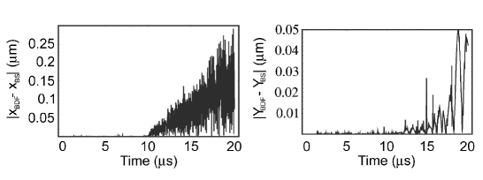
Figure 2: This figure shows the absolute value of the difference between the Bulirsch-Stoer and BDF numerical estimates of the x- and y-components of the position of an ion shuttled along a linear path. As we can see, the disagreement in the numerical estimates increase with time.

We use the Bulirsch-Stoer Method and the Backward Difference Formulae to numerically evaluate the solution to a simple harmonic oscillator differential equation for the time interval $(t=0$ s, $t=0.01$ s$)$ with $\omega/2\pi=1$ MHz. We first observe that the BDF method takes more steps than the Bulirsch-Stoer Method; 958331 steps as compared to 207422. The second observation is that the average error increases monotonically with the number of steps taken with fixed error goals. This result is shown in Fig. 3 as plots of the absolute difference between the ODE solver method and the exact solution as a function of time. From Fig. 3, if we ignore the spurious errors    due to the interpolation process, the error of the Bulirsch-Stoer method is much smaller than that of the BDF method and supports our conjecture that an ODE solver that can cross the interval in less steps will be more accurate than an ODE solver that crosses the interval in more steps.

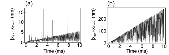
Figure 3: (a) depicts the absolute value of the deviation of the numerical estimate derived from the Bulirsch-Stoer method and the exact solution of the equations of motion of a simple harmonic oscillator. There are several spurious peaks in the graph and these are due to inaccuracies in the interpolation process to fit the generated nodes and are not errors from the numerical solution. If we ignore these spurious peaks, we note that the average error increases linearly with time and is due to the quadratic potential. (b) depicts the absolute value of the deviation of the numerical estimate derived from the BDF method and the exact solution. Unlike (a), there are no spurious peaks because the BDF method generates more nodes which implies that the nodes are closer together and thus the interpolation process is more accurate. We note that in both figures the average error increases monotonically with time and the error of the solution derived from the Bulirsch-Stoer method is much smaller than the error derived from the BDF method.

We used the Bulirsch-Stoer method to simulate ion motion during shuttling because of the superior accuracy of this method for obtaining a numerical solution for an ion’s trajectory and the superior computational efficiency of this method. Note here that our observations pertain specifically to our particular ion trap geometry (see section 5) and our specific local error tolerances. It is possible that some other ODE solver may be more effective depending on the ion trap geometry as well as the computational resources available. Although the above analysis implies that an ODE solver with fewer steps has superior accuracy, the intermediate motion of the ion between nodes is not accessible.

3 Theoretical Description of Shuttling Atomic Ions

So far, we have described the means by which it is possible to calculate the effective electric potential at the position of the ions in an ion trap array, and also the classical trajectories that those ions will take when the voltages on the control electrodes are changed with time. The goal is to develop a system that allows ions to be moved to arbitrary locations within the trap array in a perfectly reliable manner. In addition, the ions should carry and store quantum information both before and after each shuttling operation. This indicates the need to identify those shuttling operations which keep the ions trapped and cold enough to perform quantum gate operations, all the while providing maximum speed of operation. In this section, we develop a general theoretical model of the shuttling process. Our model focuses on the case in which the motion of the ion in the trap along the pathway of the ion is affected. We have worked out the model in a rather complete fashion as a reference for future work and have applied it to several possible shuttling time profiles. Rather than just treating a simple model considering only the first vibrational state, we calculate the general case that may be applied to a much broader context. The model is then used to identify those constraints that ensure reliable transport of ions. By identifying such parameters the reader can construct effective shuttling protocols for a variety of situations. For those who wish to skip the details of the theoretical analysis, the key results are presented in section 3.2.5, just prior to the section detailing how these results can be used to evaluate various shuttling procedures. A similar theoretical analysis of shuttling has recently been given by Ref. [42]. Furthermore, Ref. [43] discussed the application of control theory to single ion transport. The analysis given here emphasizes the importance of the inertial forcing of shuttled ions at the beginning and end of the protocol, as well as the possibility of significant parametric heating of the ion even for slow shuttling speeds.

3.1 The Shuttling Process

The rf Paul linear ion trap works by creating an effective potential near the center of the trap that is quadratic in all three coordinate directions. The transverse trap is produced by the rf ponderomotive potential and is symmetric and perfectly harmonic near the trap minimum, while the trap along the shuttling pathway is created by applying voltages to segmented control electrodes. This potential is also harmonic to a very good approximation. A shuttling operation involves changing the voltages on the control electrodes in time, so that the potential minimum along the ion pathway is translated from the initial ion position to the desired final position.

It is helpful to begin by considering the electric field along the ion pathway in the vicinity of the ion. The one-dimensional harmonic potential along the trap axis corresponds to a linearly-varying field,

$$E(x)=-{\cal E}x,$$ (21)

with its stable equilibrium point at $x=0.$ This field is the result of the potential difference between the nearest control electrodes that are held at or below ground, and the neighboring control electrodes. The shuttling operation described above corresponds to introducing a potential difference between the control electrodes. This voltage difference results in a nearly spatially-uniform, time-dependent electric field superimposed on the original trapping field and pointing in the direction of shuttling. The resulting electric field,

$$E(x,t)=-{\cal E}x+E(t)=-{\cal E}(x-x_{0}(t)),$$ (22)

now has a stable equilibrium point $x_{0}(t)=\frac{E(t)}{{\cal E}},$ that varies with time. The resulting electric potential is given by

$$V(x,t)={\cal E}\left(\frac{1}{2}x^{2}-x_{0}(t)x\right)+V_{0}(0,t),$$ (23)

where $V_{0}$ represents the (time-varying) potential at $x=0.$ We choose the zero of the electric potential to be located at $x_{0}(t)$, i.e. $V(x=x_{0}(t),t)=0,$ and therefore,

$$V_{0}(0,t)=\frac{1}{2}{\cal E}x_{0}^{2}(t)=\frac{E^{2}(t)}{2{\cal E}}.$$ (24)

In practice, this time-dependent potential can be introduced during the shuttling process by continually raising (lowering) the voltages on the electrodes behind (ahead of) the moving ion (see Sec. 5.2).

Finally, we obtain the expression for the potential energy in the trap frame as a function of $x$ and $t$,

$$U(x,t) = \frac{1}{2}e{\cal E}\left(x^{2}-2x_{0}(t)x+x_{0}^{2}(t)\right)$$ (25)

$$= \frac{1}{2}m\omega^{2}(x-x_{0}(t))^{2},$$ (26)

where we have identified ${\cal E}=\frac{m\omega^{2}}{e}$ (See Fig. 4).

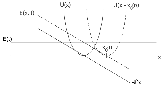
Figure 4: Schematic drawing showing the relationship between the initial electric field $-{\cal E}x$ creating the axial trap, the time-dependent forcing field, $E(t)$, and the resulting field $E(x,t),$ along with the potentials at times 0 and $t$ and the location of the minimum, $x_{0}(t)$.

This translating potential can be thought of as a moving bowl for the purpose of carrying a marble from place to place. Quantum mechanically, the last term in Eq. 25 does not induce transitions between states and merely produces an overall phase factor in the quantum state because it is independent of the position operator $x$ (see Eq. 42). Therefore, the problem of shuttling atomic ions and determining the effect of shuttling on their motional states is equivalent to the problem of solving for the transitions induced in a harmonic oscillator being forced by a uniform field, $eE(t)=m\omega^{2}x_{0}(t).$ The forcing field determines the location of the instantaneous potential minimum of the moving ion trap.

We now examine the case when a cooled ion is shuttled a distance $L$ over a time $T$, so that $x_{0}(t)=0$ for $t<0$ and $x_{0}(t)=L$ for $t>T$. The trajectory of the potential minimum $x_{0}(t)$ is directly related to the time-dependent voltage difference $\Delta V_{cap}(t)$ applied to the relevant control electrodes. That is, we expect that

$$x_{0}(t)=E(t)\frac{e}{m\omega^{2}}=\eta(x_{0}(t))\frac{\Delta V_{cap}(t)}{d}\frac{q}{m\omega^{2}},$$ (27)

where $\eta(x)$ is a unitless geometrical function relating the control electrode voltage difference to the electric field at position $x$, and $d$ is the characteristic center-to-center distance between neighboring electrodes. Therefore, Eq. 27 tells us that from a knowledge of the desired functional form for the trajectory $x_{0}(t)$ and the position dependent geometrical function $\eta(x)$ the required voltage differences $\Delta V_{cap}(t)$ across the control electrodes can be determined. Functional forms for the trajectories of the potential minimum include piecewise linear functions, sinusoids, and other transcendental functions such as the hyperbolic tangent function [26]. We will therefore consider the following three potential minimum time profiles for translating the harmonic potential: linear ($x_{0l}(t)$), sinusoidal ($x_{0s}(t)$), and hyperbolic tangent ($x_{0t}(t)$), defined as

$$x_{0l}(t) = L\frac{t}{T}(H(t)-H(t-T))+LH(t-T),$$ (28)

$$x_{0s}(t) = \frac{L}{2}\left(1-\cos\left(\frac{\pi t}{T}\right)\right)(H(t)-H(t-T))+LH(t-T),$$ (29)

$$x_{0t}(t) = \frac{L}{2}\frac{\left(\tanh\left(N\frac{2t-T}{T}\right)+\tanh(N)\right)}{\tanh(N)}(H(t)-H(t-T))+LH(t-T).$$ (30)

In these expressions, $H(t)$ is the Heaviside step function, and the parameter $N$ in the hyperbolic tangent potential minimum time profile characterizes the translation rate at the midpoint of the motion and also determines the magnitude of the discontinuity in the velocity of the potential at the beginning and end of the protocol (Fig. 5). For $N>1$, the time between $10\%$ and $90\%$ of the transition is $\sim T/N$ and the velocity discontinuity is $\sim(4L/T)Ne^{-2N}$

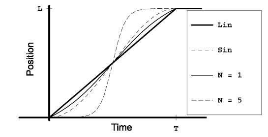
Figure 5: Plot of the position of the potential minimum of the trap versus time, when the potential minimum time profile is linear, sinusoidal and a hyperbolic tangent (N =1 and N = 5). The variables $L$ and $T$ represent the total shuttling distance and time, respectively.

Any time dependence of $\omega$ will also enter into the functional form of $x_{0}(t),$ as can be seen from Eq. 27. We can better separate the influence of fluctuations in the frequency from that of the time-dependent electric field, $E(t),$ by transforming to the rest frame of the moving potential. The position coordinate becomes $s=x-x_{0}(t)$ and a pseudo-forcing term, $m\ddot{x}_{0}s,$ is simultaneously introduced into the potential energy because the reference frame of the moving potential minimum will not be inertial. The potential energy from Eq. 25 then becomes

$$U(s,t)=\frac{1}{2}m\omega^{2}(t)s^{2}+m\ddot{x}_{0}(t)s.$$ (31)

The potential $U(s,t)$ still describes a forced, parametric harmonic oscillator, but the frequency variation of the potential and the forcing term due to the translation of the potential are now separate. What is more, the forcing term no longer includes the net displacement of the oscillator $x_{0}(t)$. Instead, it is solely a result of the inertial force on the ion due to an acceleration in the transport of the potential. If the potential were simply accelerating at a constant rate the minimum could be redefined, as was done for the potential in the lab frame (Eq. 25). However, a shuttling process necessarily involves both a start from rest and a bringing to rest of the harmonic potential. Therefore, the ion will at the least receive two kicks or pushes away from the instantaneous potential minimum. This can be seen clearly by examining the second derivative of the representative time profiles for the potential minimum in the lab frame, given in Eq. 28. After invoking the properties of the derivative of a delta function, we get:

$$\ddot{x}_{0l}(t) = \frac{L}{T}(\delta(t)-\delta(t-T)),$$ (32)

$$\ddot{x}_{0s}(t) = \frac{L\pi^{2}}{2T^{2}}\cos\left(\frac{\pi t}{T}\right)(H(t)-H(t-T)),$$ (33)

$$\ddot{x}_{0t}(t) = -L\frac{4N^{2}}{T^{2}}\coth(N)\frac{\tanh\left(N\frac{2t-T}{T}\right)}{\cosh^{2}\left(N\frac{2t-T}{T}\right)}(H(t)-H(t-T))+$$

$$+L\frac{N}{T}\frac{\coth(N)}{\cosh^{2}\left(N\frac{2t-T}{T}\right)}(\delta(t)-\delta(t-T)).$$

Here we see that the inertial forcing induced during a typical shuttling protocol has the general form

$$\ddot{x}_{0}(t)=A(t,T)\frac{L}{T}\left[\delta(t)-\delta(t-T)\right]+B(t,T)\frac{L}{T^{2}}\left[H(t)-H(t-T)\right],$$ (35)

where $A(t,T)$ and $B(t,T)$ are defined by the particular shuttling protocol. The delta function term, proportional to $L/T$, is associated with inertial kicks received by the shuttled ion due to the sudden start-up and completion of the shuttling protocol. The step function term, proportional to $L/T^{2}$, is associated with the inertial forcing due to the acceleration and deceleration of the shuttling potential during the shuttling protocol. The linear potential minimum time profile $(B(t,T)=0)$ is seen to provide two large ‘kicks’ of magnitude $L/T$ but in opposite directions. On the other hand, it produces no push on the ion except at the start and finish of the protocol. The sinusoidal potential minimum time profile $(A(t,T)=0)$ has zero velocity at the start and end of the shuttling, but it does provide a steady push proportional to $L/T^{2}$ over the duration of the shuttling, first back and then forward. The hyperbolic tangent potential minimum time profile has both features of the other profiles, to a degree controlled by the parameter $N$. A large value of $N$ results in a smooth beginning and ending to the process, but a large backwards and then forward pushing in the middle. A small $N$ produces the opposite result.

We also need to introduce an appropriate model for frequency variations of the potential as the ion is carried along during the shuttling procedure. In general, we want to consider frequency variations of the type,

$$\omega(t)^{2}=\omega_{0}^{2}(1-f(t)).$$ (36)

We will assume in our analysis that the function $f(t)$ is zero at the beginning and ending of the shuttling process. For convenience, we will consider perturbations extending from $t=-T/2$ to $t=T/2,$ and then adjust the time scale so that the shuttling and frequency variation models match. Two types of perturbation will be considered. First, a ‘short-step’ model is considered where the trapping potential is weakened by decreasing the voltage on the electrode in front of the ion and then strengthened by increasing the voltage on the electrode behind the ion. This will result in a potential for which the trap frequency will gradually decrease and then increase. The second type of perturbation to be considered is that of a fluctuating trap frequency. In this case, the ion can be thought of as being forced in one direction by a continuously increasing electric field. As a result, the frequency experienced by the ion can be modulated due to the fluctuating strength of the “static” trapping fields as the ion passes gaps or other changes in the electrode structure. This fluctuation could affect the trapping potential in either the transverse or longitudinal directions. Another source of frequency variation in the potential of this type might be low frequency noise from the control electrodes used to trap and shuttle the ions. Both types of perturbations can be modeled by the same function,

$$f(t)=g\cos\left\{(M+1/2)\frac{2\pi t}{T}\right\}.$$ (37)

When the parameter $M$ is set to zero this forcing produces a decrease and then increase in the frequency over the duration of the shuttling protocol, as required for the ‘short-step’ model. For $M$ an integer, the sinusoidal variation of the potential has $M+1/2$ “cycles” throughout the shuttling, which may correspond to the number of periodic structures in the trap electrode array. These two models for the frequency variation of the shuttling potential are illustrated in Fig. 6.

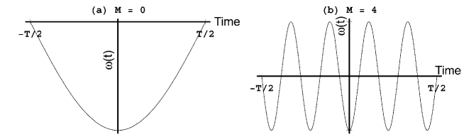
Figure 6: Plots of the ‘single-step’ (M = 0 in Eq. 37) and ‘long distance’ (M = 4) models for the frequency variation in the shuttling potential. The vertical axis ranges from $\omega_{0}^{2}(1-g)$ to $\omega_{0}^{2}(1+g)$.

The parameter $g$, known as the frequency modulation depth, characterizes the fractional variation in the square of the frequency of the potential. In order to optimize the shuttling process, we will first examine the effect of arbitrary frequency fluctuations and inertial forcing on the final motional state of shuttled ions, and then apply the results to the models outlined above.

3.2 The Forced Parametric Oscillator

The problem of the forced harmonic oscillator has been solved quantum mechanically by Husimi [44] and Kerner [45], independently. Husimi’s solution includes the effects of both inertial forcing and frequency variation on the oscillator. We seek expressions for the average final motional state, $\langle n\rangle$ and the variance in the distribution about the mean, $\langle\Delta n^{2}\rangle,$ following Husimi’s solution. In particular, we will first examine the solution to the time-dependent Schrödinger’s equation and show that it can be separated into a solution for the unforced parametric oscillator and a solution for the forced parametric oscillator. Then we will seek solutions for those two cases using the method of generating functions. This approach starts from the basic observation that the Hermite polynomials from which the eigenfunctions of the harmonic oscillator are constructed can be used to obtain a power series expansion of a generating function. A propagator is used to describe the time evolution of the oscillator system. The generating functions of the individual wavefunctions are used in conjunction with this approach to obtain generating functions for the transition amplitudes and transition probabilities relating the initial and final states of the system. The method of generating functions is a powerful method for our purposes, since the desired quantities are not the individual matrix elements describing the likelihood of ending up in a particular state, but the average value of $n(T)$, which is given by the sum over all possible final states at time $T$. This sum can be obtained by manipulating the generating function directly.

3.2.1 Solving Schrödinger’s equation

Starting from the one-dimensional Schrödinger’s equation for $\psi(s,t)$ in the frame of the potential minimum,

$$\imath\hbar\frac{\partial\psi(s,t)}{\partial t}=-\frac{\hbar^{2}}{2m}\frac{\partial^{2}\psi(s,t)}{\partial s^{2}}+\frac{1}{2}m\omega^{2}(t)s^{2}\psi(s,t)+m\ddot{x}_{0}(t)s\psi(s,t),$$ (38)

a second coordinate transformation is introduced, so that

$$s^{\prime} = s-\xi(t)$$

$$\frac{\partial\psi(s,t)}{\partial t} = \frac{\partial\psi(s^{\prime},t)}{\partial t}-\dot{\xi}(t)\frac{\partial\psi(s^{\prime},t)}{\partial s^{\prime}}$$

$$\frac{\partial^{2}\psi(s,t)}{\partial s^{2}} = \frac{\partial^{2}\psi(s^{\prime},t)}{\partial s^{\prime 2}}.$$ (39)

The transformation, $\psi(s^{\prime},t)=\phi(s^{\prime},t)e^{ims^{\prime}\dot{\xi}/\hbar}$ is then introduced to eliminate the first order spatial derivative arising in the second line of Eq. 3.2.1, and upon substitution into Eq. 38 results in the following equation for $\phi(s^{\prime},t):$

$$i\hbar\frac{\partial\phi(s^{\prime},t)}{\partial t} = -\frac{\hbar^{2}}{2m}\frac{\partial^{2}\phi(s^{\prime},t)}{\partial s^{\prime 2}}+\frac{1}{2}m\omega^{2}(t)s^{\prime 2}\phi(s^{\prime},t)$$ (40)

$$+m\left((\ddot{\xi}+\ddot{x}_{0})+\omega^{2}(t)\xi\right)s^{\prime}\phi(s^{\prime},t)-$$

$$-m/2\left(\dot{\xi}^{2}+\dot{x}_{0}^{2}-\omega^{2}(t)\xi^{2}-2\ddot{x}_{0}\xi\right)\phi(s^{\prime},t).$$

The first line of Eq. 40 is the wave equation for the unforced parametric harmonic potential, which has solutions given by $\chi(s^{\prime},t).$ The coefficient of $\phi(s^{\prime},t)$ in the third line on the RHS is independent of coordinate $s^{\prime}$, and gives rise to a simple time-dependent phase factor. Finally, the second line on the RHS can be eliminated by choosing the transformation coordinate, $\xi$, to be the solution of the equation,

$$\ddot{\xi}+\omega^{2}(t)\xi+\ddot{x}_{0}=0.$$ (41)

This is the classical equation of a forced, parametric harmonic oscillator, where $\xi$ is identified as the classical position of an ion relative to the moving potential minimum.

Combining the observations made above, we see that the wave equation for $\phi(s^{\prime},t)$ is in fact separable, and its solution can be written down in terms of the solutions $\chi(s^{\prime},t)$ of the unforced parametric oscillator equation, and the phase factor from the remaining time-dependent terms in Eq. 40:

$$\phi(s^{\prime},t)=\chi(s^{\prime},t)\exp\left\{\frac{i}{\hbar}\int_{t_{0}}^{t}m/2\left(\dot{\xi}^{2}+\dot{x}_{0}^{2}-\omega^{2}(t)\xi^{2}-2\ddot{x}_{0}\xi\right)dt\right\}.$$ (42)

Recalling the canonical transformation introduced above, the full solution to the time-dependent wave function, $\psi(s^{\prime},t)$, is then found to be

$$\psi(s^{\prime},t)=\chi(s^{\prime},t)\exp\left\{\frac{i}{\hbar}ms^{\prime}\dot{\xi}+\frac{i}{\hbar}\int_{t_{0}}^{t}m/2\left(\dot{\xi}^{2}+\dot{x}_{0}^{2}-\omega^{2}(t)\xi^{2}-2\ddot{x}_{0}\xi\right)dt\right\}.$$ (43)

Therefore, the problem of finding the wavefunction of the forced, parametric oscillator as a function of time has been reduced to one of finding the quantum mechanical solution, $\chi(s^{\prime},t)$, for the unforced parametric oscillator and the classical solution, $\xi(t)$, of the forced, parametric oscillator. As described in the introduction to this section, we wish to obtain the generating functions for the matrix elements describing the transition from the initial to the final state of the ion. This is facilitated by a propagator approach to describe the time-evolution of the quantum mechanical state of the ion.

3.2.2 The method of generating functions

We begin our derivation of the generating functions for the transition probabilities in unforced and forced parametric oscillators by recalling the propagator for the simple harmonic oscillator [46]:

$$\psi(x,t)=\int K_{sho}(x,t|x^{\prime},t^{\prime})\psi(x^{\prime},t^{\prime})dx^{\prime}.$$ (44)

The propagator $K_{sho}(x,t|x^{\prime},t^{\prime})$ satisfies the time-dependent Schrödinger’s equation for the harmonic oscillator, and is given by [46]

$$K_{sho}(x,t|x^{\prime},t^{\prime}) = \sqrt{\frac{m\omega_{0}}{2\pi i\hbar\ \sin(\omega_{0}\Delta t)}}$$ (45)

$$\times \exp\left\{\frac{im\omega_{0}}{2\hbar\sin(\omega_{0}\Delta t)}\left(x^{2}\cos(\omega_{0}\Delta t)-2xx^{\prime}+{x^{\prime}}^{2}\cos(\omega_{0}\Delta t)\right)\right\},$$

where $\Delta t=t-t^{\prime}.$ The probability amplitude for the simple harmonic oscillator, initially in a pure state $\psi(x^{\prime},t^{\prime})$, to be in the $n$-th eigenstate at time $t$ is then given by a double integral over $x$ and $x^{\prime}$

$$b_{n}(t,t^{\prime})=\int\int\psi_{n}^{*}(x)K_{sho}(x,t|x^{\prime},t^{\prime})\psi(x^{\prime},t^{\prime})\,dx\,dx^{\prime}.$$ (46)

The probabilities for the simple harmonic oscillator to be in the $n$-th state are then

$$P_{n}(t,t^{\prime})=|b_{n}(t,t^{\prime})|^{2}.$$ (47)

In the case that the particle is initially in the $k$-th eigenstate of the harmonic oscillator, the expressions for the probability and probability amplitude of the system being in the $n$-th state in Eqs. 47 and 50 can be thought of as transition probabilities for the evolving system. Of course, for a stationary quadratic potential with a fixed frequency, the transition probabilities would be

$$P_{nk}(t,t^{\prime})=|b_{nk}(t,t^{\prime})|^{2}=\delta_{nk}.$$ (48)

However, when the ion is shuttled and experiences a nonuniform acceleration and/or a changing trap frequency, we can expect transitions from one eigenstate of the harmonic oscillator to another. The key to determining those transition probabilities is the propagator $K(x,t|x^{\prime},t^{\prime})$ for the shuttling potential, which is a solution of the Schrödinger’s equation for the shuttling potential:

$$\imath\hbar\frac{\partial K(x,t|x^{\prime},t^{\prime})}{\partial t}=-\frac{\hbar^{2}}{2m}\frac{\partial^{2}K(x,t|x^{\prime},t^{\prime})}{\partial x^{2}}+\left(\frac{1}{2}m\omega^{2}x^{2}+m\ddot{x}_{0}(t)x\right)K(x,t|x^{\prime},t^{\prime}),$$ (49)

and satisfies $K(x,t^{\prime}|x^{\prime},t^{\prime})=\delta(x-x^{\prime})$. Assuming this function is known, the transition amplitudes for the ion to begin in the $k$-th state of the harmonic potential at time $t^{\prime}$ and then after being shuttled to end up in the $n$-th state of the harmonic potential at time $t$ are

$$b_{nk}(t,t^{\prime})=\int\int\psi_{n}^{*}(x)K(x,t|x^{\prime},t^{\prime})\psi_{k}(x^{\prime})\,dx\,dx^{\prime}.$$ (50)

This expression for the transition amplitudes can be used to construct a generating function, $B(u,v),$ for the transition amplitudes of the shuttled ion. We start by using the known generating function for the eigenfunctions of a simple harmonic oscillator with frequency $\omega_{0}$ (e.g., Husimi [44], Eq. 4.6):

$$\sqrt{\alpha}e^{-u^{2}+2\alpha ux-\alpha^{2}x^{2}}=\sum_{n}\sqrt{\frac{\sqrt{\pi}2^{n}}{n!}}u^{n}\psi_{n}(\alpha x),$$ (51)

where $\alpha=\sqrt{m\omega_{0}/\hbar}$ and $|u|\leq 1.$ We multiply both sides of Eq. 50 by $\sqrt{\frac{\pi 2^{n+k}}{n!k!}}u^{k}v^{n}$ and then by summing both sides over $k$ and $n$, we have

$$B(u,v) = \sum_{k,n}\sqrt{\frac{\pi 2^{n+k}}{n!k!}}u^{k}v^{n}b_{nk}(t,t^{\prime})$$ (52)

$$= \alpha\int dx\,dx^{\prime}K(x,t|x^{\prime},t^{\prime})\exp\left\{-u^{2}-v^{2}+2\alpha(ux^{\prime}+vx)-\alpha^{2}({x^{\prime}}^{2}+x^{2})\right\}.$$

Notice that the generating function $B(u,v)$ is a function of the initial and end times of the shuttling protocol as well. Once the propagator for the potential is known, any particular transition amplitude can be obtained from this generating function by expanding it about the parameters $u$ and $v$ and reading off the transition amplitude $b_{nk}$ from the coefficient of the $u^{k}v^{n}$ term in the expansion. A similar generating function can be developed for the transition probabilities by treating the probabilities $P_{nk}$ as coefficients in a double power series in $u$ and $v$, and then using the integral obtained for $b_{nk}$ in Eq. 50 so that

$$P(u,v) = \sum_{k,n}u^{k}v^{n}P_{nk}(t,t^{\prime})=\sum_{k,n}u^{k}v^{n}|b_{nk}(t,t^{\prime})|^{2}$$ (53)

$$= \int\int\int\int dx\,dx^{\prime}\,dy\,dy^{\prime}K(x,t|x^{\prime},t^{\prime})K^{*}(y,t|y^{\prime},t^{\prime})$$

$$\times \left\{\sum_{n}v^{n}\psi_{n}^{*}(\alpha x)\psi_{n}(\alpha y)\right\}\left\{\sum_{k}u^{k}\psi_{k}^{*}(\alpha x^{\prime})\psi_{k}(\alpha y^{\prime})\right\}.$$

Each term in braces in the bottom line of Eq. 53 can be replaced for $|u|,|v|\leq 1$ by the bilinear generating function (see Husimi [44], Eq. 4.4)

$$\sqrt{\frac{\alpha^{2}}{\pi(1-u^{2})}}\exp\left\{-\alpha^{2}\frac{(1+u^{2})(x^{2}+y^{2})-4uxy}{2(1-u^{2})}\right\}=\sum_{n}u^{n}\psi_{n}\left(\alpha y\right)\psi_{n}^{*}\left(\alpha x\right).$$ (54)

Making the substitution, we obtain the generating function for the transition probabilities,

$$P(u,v) = \frac{\alpha^{2}}{\pi\sqrt{(1-u^{2})(1-v^{2})}}\int\int\int\int dx\,dx^{\prime}\,dy\,dy^{\prime}K(x,t|x^{\prime},t^{\prime})K^{*}(y,t|y^{\prime},t^{\prime})$$ (55)

$$\times \exp\left\{-\alpha^{2}\left(\frac{(1+u^{2})(x^{2}+y^{2})-4uxy}{2(1-u^{2})}+\frac{(1+v^{2})({x^{\prime}}^{2}+{y^{\prime}}^{2})-4vx^{\prime}y^{\prime}}{2(1-v^{2})}\right)\right\}.$$

Again, once the propagators for the shuttling potentials are known, the generating function for the transition probabilities can be obtained by carrying out the fourfold integral on the RHS of Eq. 55.

One can obtain directly the average final state of the shuttled ion by manipulating this expression as follows:

$$\left.\frac{\partial P(u,v)}{\partial v}\right|_{v=1}=\sum_{k}u^{k}\sum_{n}nP_{nk}(t,t^{\prime})=\sum_{k}u^{k}\langle n_{k}\rangle.$$ (56)

By expanding the term on the LHS in powers of $u$, one can read off for an ion which started in the $k$-th eigenstate of the trapping potential its average final state, defined to be $\langle n_{k}\rangle.$ If we make the further assumption that the oscillator started out in the ground state, $k=0$, we only need the term in the expansion which has no dependence on $u$. We can find this term easily by setting $u=0,$ so that only that part of $P(u,v)$ which doesn’t depend on $u$ survives. Thus, the average final state for an ion which started in the zeroth eigenstate of the trapping potential, $\langle n_{0}\rangle,$ is found by setting $u=0$ in the expression on the LHS of Eq. 56,

$$\langle n_{0}\rangle=\sum_{n}nP_{n0}(t,t^{\prime})=\left.\frac{\partial P(0,v)}{\partial v}\right|_{v=1}.$$ (57)

We can also find the distribution of the wavefunction about the mean for the final motional state by manipulating the generating function, $P(u,v)$. For an arbitrary initial state, $k$, we can find the average value of $n(n-1)=n^{2}-n$, defined as $\langle n^{2}_{k}\rangle-\langle n_{k}\rangle$, by taking the second derivative of the generating function with respect to $v$, and then evaluating it for $v=1,$

$$\left.\frac{\partial^{2}P(u,v)}{\partial v^{2}}\right|_{v=1}=\sum_{k}u^{k}\sum_{n}n(n-1)P_{nk}(t,t^{\prime})=\sum_{k}u^{k}\left(\langle n_{k}^{2}\rangle-\langle n_{k}\rangle\right),$$ (58)

from which we can easily obtain the distribution of the final ion state about the mean, $\langle n_{k}^{2}\rangle-\langle n_{k}\rangle^{2}$. In the particular case that $k=0$, we can obtain the distribution about the mean, $\langle\Delta n_{0}^{2}\rangle,$ directly from derivatives with respect to $v$ of the generating function $P(0,v)$ as in Eq. 57 above,

$$\langle\Delta n_{0}^{2}\rangle = \langle n_{0}^{2}\rangle-\langle n_{0}\rangle^{2}$$ (59)

$$= \left.\frac{\partial^{2}P(0,v)}{\partial v^{2}}\right|_{v=1}+\left.\frac{\partial P(0,v)}{\partial v}\right|_{v=1}-\left(\left.\frac{\partial P(0,v)}{\partial v}\right|_{v=1}\right)^{2}.$$

Thus, the method of generating functions is a powerful way to obtain the average final state and the distribution about the mean of the final state of a forced parametric oscillator. In the particular case that the ion was initially in the ground state, these values can be obtained directly from first and second order derivatives of $P(0,v)$ with respect to the parameter $v$, with $v$ subsequently set equal to 1. These values can be written down in closed form expressions if the propagator for the forcing potential is known and the integrals for the generating functions are solvable.

3.2.3 Classical solutions for the unforced and forced parametric oscillator

As we showed in Sec. 3.2.1, the quantum mechanical solutions of the unforced and forced harmonic oscillator problem are expressed in terms of the classical quantities describing the motion of these systems. Therefore, we turn our attention to the solution of the classical forced parametric oscillator equation, given in Eq. 41. We specify $\xi$ as that solution of the forced parametric oscillator for which the initial conditions $\xi(t_{0},t_{0})=\dot{\xi}(t_{0},t_{0})=0$ hold in the frame of the moving potential. This will serve to cause the phase factor in Eq. 43 to vanish at time $t_{0}$. This solution can be obtained by considering first the homogeneous equation, which is the unforced parametric oscillator equation,

$$\ddot{X}=-\omega(t)^{2}X.$$ (60)

There exist two independent solutions $X_{1}(t)$ and $X_{2}(t)$ of Eq. 60, which satisfy the initial conditions {$X(t_{0})=0,\dot{X}(t_{0})=1$} and {$X(t_{0})=1,\dot{X}(t_{0})=0$}, respectively. These solutions have the property that, for any time $t>t_{0}$

$$X_{1}X_{2}-X_{2}X_{1}=0;\hskip 7.22743pt\mbox{and}\hskip 7.22743pt\dot{X}_{1}X_{2}-X_{1}\dot{X}_{2}=1,$$ (61)

where the first property is obvious and the second property is derived, using Eq. 60 and the first property, as follows:

$$X_{2}(t)\ddot{X}_{1}(t)-X_{1}(t)\ddot{X}_{2}(t) = -\omega(t)^{2}\left(X_{1}(t)X_{2}(t)-X_{2}(t)X_{1}(t)\right)=0$$

$$\frac{d}{dt}\left(\dot{X}_{1}(t)X_{2}(t)-X_{1}(t)\dot{X}_{2}(t)\right) = 0$$

$$\dot{X}_{1}(t)X_{2}(t)-X_{1}(t)\dot{X}_{2}(t) = \dot{X}_{1}(t_{0})X_{2}(t_{0})-X_{1}(t_{0})\dot{X}_{2}(t_{0})=1.$$ (62)

Therefore, these solutions can be used to construct a one-dimensional Green’s function,

$$G(t,t^{\prime})=X_{1}(t)X_{2}(t^{\prime})-X_{1}(t^{\prime})X_{2}(t),$$ (63)

for $t\geq t^{\prime}\geq t_{0}$ which has the properties

$$G(t^{\prime},t^{\prime})=0;\hskip 7.22743pt\mbox{and}\hskip 7.22743pt\frac{dG(t^{\prime},t^{\prime})}{dt}=1.$$ (64)

This Green’s function, which has the dimensions of time, can be shown to be [47] the solution of the parametric oscillator equation with delta function forcing,

$$\ddot{G}(t,t^{\prime})+\omega(t)^{2}G(t,t^{\prime})=\delta(t-t^{\prime}),$$ (65)

where $G(t,t^{\prime})=0,$ for $t<t^{\prime}$ to satisfy causality. The solution for $G$ when $t>t^{\prime}$ then represents the response of the oscillator to a unit impulse occurring at time $t^{\prime}$. In the simplest case for which the frequency of the potential is fixed at $\omega_{0}$, we have

$$X_{1}(t,t_{0};\omega_{0}) = \frac{1}{\omega_{0}}\sin(\omega_{0}(t-t_{0})),$$

$$X_{2}(t,t_{0};\omega_{0}) = \cos(\omega_{0}(t-t_{0})),$$

$$G(t,t^{\prime}) = \frac{1}{\omega_{0}}\sin(\omega_{0}(t-t^{\prime})).$$ (66)

Once the appropriate $G(t,t^{\prime})$ has been obtained, the solution for $\xi(t,t_{0})$ satisfying Eq. 41 can now be constructed as follows:

$$\xi(t,t_{0}) = -\int_{t_{0}}^{t}\ddot{x}_{0}(t^{\prime})G(t,t^{\prime})dt^{\prime}$$

$$\dot{\xi}(t,t_{0}) = -\int_{t_{0}}^{t}\ddot{x}_{0}(t^{\prime})\frac{\partial G(t,t^{\prime})}{\partial t}dt^{\prime}.$$ (67)

The classical energy gain of the ion due to forcing, relative to the characteristic energy of the harmonic potential, is therefore

$$\Upsilon(t,t_{0})=\frac{m}{2\hbar\omega(t)}\left(\omega(t)^{2}\xi(t,t_{0})^{2}+\dot{\xi}(t,t_{0})^{2}\right).$$ (68)

In order to isolate the influence of the frequency variation on the shuttled ion’s energy, we switch the role of $t$ and $t_{0}$ in Eq. 3.2.3. This can be understood as the motion of the ion when the sequence of frequency variation is reversed. The need for this arises from the fact that for the forced motion the energy gain is not only a function of the end time, but also the initial time. Therefore, we have [44],

$$\xi(t_{0},t) = -\int_{t}^{t_{0}}\ddot{x}_{0}(t^{\prime})G(t_{0},t^{\prime})dt^{\prime}$$ (69)

$$\dot{\xi}(t_{0},t) = \frac{\partial\xi(t_{0},t)}{\partial t_{0}}=-\int_{t}^{t_{0}}\ddot{x}_{0}(t^{\prime})\frac{\partial G(t_{0},t^{\prime})}{\partial t_{0}}dt^{\prime},$$ (70)

where the Green’s function is now non-zero for times earlier than the time of the impulse, that is, for $t_{0}<t^{\prime}$. The energy gain for the reversed forced motion is therefore

$$\Upsilon(t_{0},t)=\frac{m}{2\hbar\omega(t)}\left(\omega(t)^{2}\xi(t_{0},t)^{2}+\dot{\xi}(t_{0},t)^{2}\right).$$ (71)

For a constant frequency potential this reversed motion results in the same energy gain as does the forward motion, and $\Upsilon(t,t_{0})-\Upsilon(t_{0},t)=0.$ However, in general when the frequency is time-dependent, $\Upsilon(t,t_{0})-\Upsilon(t_{0},t)\neq 0$. The generating functions for the transitions induced in the unforced and forced parametric oscillator which we obtain in the next section depend precisely on the dimensionless energies characterizing the classical energy gain of these systems.

3.2.4 Transition probabilities for the unforced and forced parametric oscillator

Since we wish to solve the unforced parametric oscillator problem first, we work in the reference frame of the minimum of the potential used to shuttle the trapped ion. It is assumed that the ion starts out at time $t_{0}$ in a pure eigenstate, $\psi_{k}(s_{0},t_{0}),$ of a harmonic oscillator of constant frequency $\omega_{0}$, and that it ends up in a potential well of the same frequency at time $t$ and position $s$ relative to the potential minimum in some superposition of eigenstates. The connection between the final state of the particle and its initial state can be expressed in terms of the propagator $K(s,t|s_{0},t_{0}),$ for the shuttling potential. We begin by returning to the propagator for the simple harmonic oscillator, which corresponds to a shuttling potential moving at constant velocity and keeping a constant frequency $\omega_{0}$, (see Eq. 45)

$$K_{sho}(s,t|s_{0},t_{0}) = \sqrt{\frac{\alpha^{2}}{2\pi i\sin(\omega_{0}\Delta t)}}$$ (72)

$$\times \exp\left\{\frac{im\omega_{0}}{2\hbar\sin(\omega_{0}\Delta t)}\left(s^{2}\cos(\omega_{0}\Delta t)-2ss_{0}+s_{0}^{2}\cos(\omega_{0}\Delta t)\right)\right\},$$

where $\Delta t=t-t_{0}.$ By comparing the functions $\sin(\omega_{0}\Delta t)/\omega_{0}$ and $\cos(\omega_{0}\Delta t)$ in Eq. 72 with solutions of the unforced parametric oscillator as given in the limiting case of Eq. 3.2.3 when the frequency is constant, we can guess that the propagator $K_{sho}$ is just a special case of the general propagator for the unforced parametric oscillator

$$K_{upo}(s,t|s_{0},t_{0})=\sqrt{\frac{m}{2\pi i\hbar X_{1}(t,t_{0})}}\exp\left\{\frac{im}{2\hbar X_{1}(t,t_{0})}\left(\dot{X}_{1}(t,t_{0})s^{2}-2ss_{0}+X_{2}(t,t_{0})s_{0}^{2}\right)\right\}.$$ (73)

Husimi ([44], Eq. 3.8) showed that this is indeed the case. Substituting this propagator into Eq. 55 results in a fourfold Gaussian integral, which can be evaluated using the formula

$$\int_{-\infty}^{\infty}\exp\left\{-\frac{\sum_{i,j}^{4}A_{ij}x_{i}x_{j}}{2}\right\}d^{4}x=\frac{(2\pi)^{2}}{\sqrt{\det\{{\bf A}\}}},$$ (74)

where the $4\times 4$ matrix A is symmetric and positive-definite. The generating function for the transition probabilities for an ion in a variable-frequency harmonic potential is then

$$P(u,v)(t,t_{0})=\sqrt{2}\left\{Q(t,t_{0})(1-u^{2})(1-v^{2})+(1+u^{2})(1+v^{2})-4uv\right\}^{-1/2},$$ (75)

where

$$Q(t,t_{0})=\frac{1}{2}\left(\omega_{0}^{2}X_{1}^{2}+\dot{X}_{1}^{2}+X_{2}^{2}+\frac{1}{\omega_{0}^{2}}\dot{X}_{2}^{2}\right).$$ (76)

The generating function in Eq. 75 is even in the following sense:

$$P(-u,-v)=P(u,v).$$ (77)

Therefore the transition probabilities are non-zero only for beginning and ending states of the same parity, resulting in the expected selection rule, $n-k=2m,$ for $m$ an integer. We have $Q\geq 1,$ where the equality holds when the frequency is constant. In a classical parametric oscillator the quantity $Q$ represents the proportional increase in energy due to frequency variation over an interval of duration $T$, averaged over all possible initial conditions having the same initial energy, $E_{\omega}(t_{0})$, so that ([44], Eq. 5.21)

$$Q(t,t_{0})=\frac{\langle E_{\omega}(T+t_{0})\rangle}{E_{\omega}(t_{0})}\geq 1.$$ (78)

We now seek the average final state $\langle n_{k}\rangle$ for an ion in such a variable-frequency harmonic potential with negligible inertial forcing, given that its initial state was the $k$-th eigenstate of the initial trap. Using Eq. 56, we determine that

$$\sum_{k}u^{k}\sum_{n}nP_{nk}(t,t_{0}) = \left.\frac{\partial P(u,v)}{\partial v}\right|_{v=1}$$ (79)

$$= \frac{1}{2(1-u)^{2}}\left((1+u)Q(t,t_{0})-(1-u)\right).$$

Expanding the function on the right in powers of $u$ allows us to identify for each initial state $k$

$$\langle n_{k}\rangle=(k+1/2)Q(t,t_{0})-1/2$$ (80)

and therefore

$$\langle E_{\omega}(T+t_{0})\rangle=\left(\langle n_{k}\rangle+\frac{1}{2}\right)\hbar\omega_{0}=Q(t,t_{0})\left(k+\frac{1}{2}\right)\hbar\omega_{0},$$ (81)

exactly corresponding to the classical result (Eq. 78). The distribution of the wavefunction about the mean is found as described at the end of Sec. 3.2.2, and is given by

$$\langle\Delta n_{k}^{2}\rangle=1/2(Q^{2}(t,t_{0})-1)(k^{2}+k+1).$$ (82)

Both $\langle n_{k}\rangle$ and $\langle\Delta n_{k}^{2}\rangle$ for the parametrically-driven ion found here are functions of the initial and final time of the shuttling through the factor $Q(t,t_{0}).$ This function in turn depends on time through the solutions $X_{1}$ and $X_{2}$. These solutions can be found analytically for certain models of the frequency variation of the shuttling potential (e.g., Eq. 37). In general, however, they need to be evaluated numerically by integrating the classical parametric oscillator equation over the duration of the shuttling protocol.

The propagator for the forced parametric oscillator can be obtained from the one for the unforced parametric oscillator by using the fact that the propagator for each is a solution of the Schrödinger’s equation for the corresponding shuttling potential. Therefore, the propagator for the unforced parametric oscillator potential (with $\ddot{x}_{0}=0$) is a solution of the Schrödinger’s equation in Eq. 49 with $\ddot{x}_{0}=0$. Not only so, but it is a solution in the coordinate system defined in Eq. 3.2.1 of the Schrödinger’s equation found in the first line of Eq. 40. The solution to that equation, the quantum mechanical version of the unforced parametric oscillator equation, was identified in the text as $\chi(s^{\prime},t)$. Any equation which $\chi(s^{\prime},t)$ satisfies is also satisfied by the propagator for the unforced parametric oscillator. Therefore, the solution for the wave function of the forced parametric oscillator obtained in terms of $\chi(s^{\prime},t)$ in Eq. 43 can also be used to obtain the propagator for the forced oscillator in terms of the propagator of the unforced oscillator

$$K_{fpo}(s^{\prime},t|s_{0}^{\prime},t_{0})=K_{upo}(s^{\prime},t|s^{\prime}_{0},t_{0})e^{\frac{i}{\hbar}ms^{\prime}\dot{\xi}+\frac{i}{\hbar}\int_{t_{0}}^{t}m/2\left(\dot{\xi}^{2}+\dot{x}_{0}^{2}-\omega(t)^{2}\xi^{2}-2\ddot{x}_{0}\xi\right)dt}.$$ (83)

Thus, the propagator for the forced parametric oscillator is given by

$$K_{fpo}(s^{\prime},t|s^{\prime}_{0},t_{0}) = \sqrt{\frac{m}{2\pi i\hbar X_{1}}}$$ (84)

$$\times \exp\left\{\frac{im}{2\hbar X_{1}}\left(\dot{X}_{1}s^{\prime 2}+X_{2}{s^{\prime}_{0}}^{2}-2s^{\prime}s^{\prime}_{0}\right)\right\}$$

$$\times \exp\left\{\frac{im}{\hbar}\left(s^{\prime}\dot{\xi}+\left[\int_{t_{0}}^{t}1/2\left(\dot{\xi}^{2}+\dot{x}_{0}^{2}-\omega(t)^{2}\xi^{2}-2\ddot{x}_{0}\xi\right)dt\right]\right)\right\}.$$

Using Eqs. 53 and 55, the generating function for the transition probabilities of an ion in the forced parametric oscillator potential can be obtained ([44], Eq. 7.13)

$$P(u,v) \equiv \sum_{n,k=0}^{\infty}u^{k}v^{n}P_{nk}(t,t_{0})$$ (85)

$$= \sqrt{\frac{2}{(1-u^{2})(1-v^{2})Q(t,t_{0})+(1+u^{2})(1+v^{2})-4uv}}$$

$$\times \exp\left[-\frac{(1-u^{2})(1-v^{2})\left\{\Upsilon(t_{0},t)\frac{1-v}{1+v}+\Upsilon(t,t_{0})\frac{1-u}{1+u}\right\}}{\left\{(1-u^{2})(1-v^{2})q(t,t_{0})+(1+u^{2})(1+v^{2})-4uv\right\}}\right].$$

This solution was extended to the case that the initial and final frequency of the forced oscillator is different in Perelomov [48]. A simpler expression is obtained if we let $u=0,$ corresponding to the case that the forced ion was initially in the ground state

$$P(0,v) \equiv \sum_{n}v^{n}P_{n0}(t,t_{0})$$ (86)

$$= \sqrt{\frac{2}{Q(1-v^{2})+(1+v^{2})}}\exp\left[-\frac{(1-v^{2})\left\{\Upsilon(t_{0},t)\frac{1-v}{1+v}+\Upsilon(t,t_{0})\right\}}{\left\{(1-v^{2})Q(t,t_{0})+(1+v^{2})\right\}}\right].$$

Again, the average final motional state of the forced ion $\langle n_{0}\rangle$ can be obtained as in Eq. 57, with the simple result,

$$\langle n_{0}(T)\rangle = \Upsilon(T,0)+\frac{1}{2}\left(Q(T,0)-1\right),$$ (87)

where we have let $t_{0}=0.$ The distribution of the ion’s wavefunction about its average motional state after the total shuttling time $T$ is found as described in Eq. 59 and is given by

$$\langle\Delta n_{0}^{2}(T)\rangle=\frac{1}{2}\left(Q^{2}(T,0)-1\right)+\left(2\Upsilon(T,0)Q(T,0)-\Upsilon(0,T)\right).$$ (88)

In the case that the frequency of the potential remains constant, these results for the final average state and state distribution reduce to the following

$$\langle n_{0}(T)\rangle = \Upsilon(T,0),$$ (89)

$$\langle\Delta n_{0}^{2}(T)\rangle = \Upsilon(T,0),$$ (90)

since $\Upsilon(t,t_{0})-\Upsilon(t_{0},t)=0$ and $Q(t,t_{0})=1$ when $\omega=\omega_{0}.$

Remarkably, the impact of the frequency variation on the final energy and dispersion of the ion is largely separable from that of the inertial forcing due to shuttling. Therefore, we can profitably treat the impact of each aspect of the shuttling process separately. For the shuttling protocols outlined in Sec. 3.1 we can obtain closed form expressions for $\langle n_{0}(T)\rangle$ and $\langle\Delta n_{0}^{2}(T)\rangle$ for the shuttled ion in the cases when the frequency is held constant or the inertial forcing is negligible. In general, the factors $\Upsilon(T,0)$ and $Q(T,0)$ must be obtained numerically by integrating the expressions in Eqs. 60, 68 and 71 over the entire shuttling interval. We emphasize that both of these quantities are obtained from a classical analysis of the unforced parametric oscillator.

Important Equations of Section 3	Equation
forced oscillator, constant frequency
propagator	45
transition probability	55
$\langle n_{0}\rangle$	57
$\langle\Delta n_{0}^{2}\rangle$	59
unforced parametric oscillator
propagator	73
transition probability	75
$Q(t,t_{0})$	76
$\langle n_{k}\rangle$	80
$\langle\Delta n_{k}^{2}\rangle$	82
forced parametric oscillator
propagator	84
transition probability	85
$\Upsilon(t,t_{0}),\Upsilon(t_{0},t)$	68, 71
$\langle n_{0}\rangle$	87
$\langle\Delta n_{0}^{2}\rangle$	90

Table 2: Table summarizing the locations of important equations in Section 3. The propagators used to calculate the transition probabilities as well the transition probabilities are given for forced oscillators and forced parametric oscillators as well as unforced parametric oscillators are given. The expectation value of the oscillator motional state as well as the variances in the motional state are given too. The subscript associated with these quantities refer to the initial state of the ion before shuttling. In the unforced parametric oscillator case, $Q(t,t_{0})$ represents the proportional increase in energy due to frequency variation over an interval of duration T, averaged over all possible initial conditions having the same initial energy (see Eq. 78). In the forced parametric oscillator case, the variable $\Upsilon(t,t_{0})$ ($\Upsilon(t_{0},t)$) represents the classical energy gain of the ion due to forcing with the sequence (reversed sequence) of the frequency variation relative to the characteristic energy of the harmonic potential. The classical motion of the ion is needed to calculate the transition probabilities in the forced and unforced parametric oscillators, so it is important to be able to accurately simulate the classical motion of trapped ions during shuttling. See section 2 and the appendix for more information on simulating the classical motion of trapped ions.

3.3 Evaluation of Shuttling Protocols

Having outlined the formalism for determining the effect of shuttling in one dimension on the motional state of the ion, we now consider the shuttling protocols developed in Sec. 3.1. We first briefly establish several criteria for effective shuttling, and then evaluate the relative merits of the shuttling protocols.

3.3.1 Shuttling criteria

Heating during the shuttling operation will typically occur along the longitudinal direction (along the shuttling path). For shuttling along a line, there is no cross talk between transverse and longitudinal heating as the longitudinal direction corresponds to a principal axis. However, transport of an ion through a junction will couple the two modes and our considerations will provide an upper limit of the change of motional state in any spatial directions after the shuttling operation.

The first and most restrictive limit on a shuttling operation is the requirement that it produce little change in the motional state of the ion, or

$$\langle n\rangle\ll 1$$ (91)

for an ion initially prepared in the ground state. Although this constraint can be met by non-adiabatic processes through appropriate phasing of the shuttling forces, it is the ultimate intention of the adiabatic limit, and for simplicity we will call it the adiabatic constraint.

A second and typically less restrictive limit is that the rms spread $s_{\mbox{rms}}$ in the ion’s final wavepacket remain small compared to the relevant optical wavelengths used in the quantum information environment. This is known as the Lamb-Dicke limit, and can be an important criterion for the effective coupling of light fields to the motion of trapped ions. For a coherent state or a thermal state of harmonic motion with mean vibrational number $\langle n\rangle$,

$$s_{\mbox{rms}}=\sqrt{\langle\psi(s,T)|s^{2}|\psi(s,T)\rangle}=\sqrt{\frac{\hbar}{2m\omega_{0}}(2\langle n\rangle+1)}\,,$$ (92)

so for an ion initially in the ground state, the Lamb-Dicke criterion can thus be written as

$$\frac{\hbar k^{2}}{2m\omega_{0}}(2\langle n\rangle+1)\ll 1\,,$$ (93)

where $k$ is the effective wave-number associated with the radiation field in the quantum gate scheme. The Lamb-Dicke limit sets a more meaningful limit on the required localization of the ion for many quantum logic gate schemes [2, 5, 15, 17, 10, 11].

A third and still less restrictive constraint is that the residual motion of the ion after shuttling does not add to the diffraction limit of the ion image. This condition is important for schemes that couple ion qubits through emitted photons that might be mode-matched into an optical fiber [7, 53]. A conservative estimate of this condition is the usual Rayleigh criterion

$$s_{\mbox{rms}}\ll\frac{0.61\lambda}{\mbox{NA}}$$ (94)

where $\lambda$ is the radiation wavelength and $\mbox{NA}<1$ is the numerical aperture of the imaging objective. This diffraction limit condition can be written in a form similar to the Lamb-Dicke criterion above:

$$0.068(NA)^{2}\frac{\hbar k^{2}}{2m\omega_{0}}(2\langle n\rangle+1)\ll 1.$$ (95)

The last, and typically least restrictive constraint is that the motion of the ion remains harmonically bound in the trap. Anharmonic wavepacket dispersion can give rise to errors in certain ultrafast quantum gate schemes [54]. This condition requires that the ion motion be localized to a region of space much smaller than the characteristic distance from ion to trap electrode $d_{\mbox{eff}}$:

$$\frac{\hbar}{2m\omega_{0}d_{\mbox{eff}}^{2}}\left(2\langle n\rangle+1\right)\ll 1.$$ (96)

Now consider those features of the shuttling process which would make it more likely to satisfy the theoretical criteria, regardless of the particular shuttling protocol used. From Eqs. 68 and 91, the adiabatic constraint favors low mass ions such as beryllium or calcium for a given trap frequency. The Lamb-Dicke and diffraction criteria favor atomic ions that feature longer-wavelength electronic transitions (Eqs. 93 and 95). In addition, for a given atom any shuttling protocol can be made faster while making it less likely for the ion to be placed into an excited state by increasing the axial trap frequency, $\omega_{0}.$ The Lamb-Dicke and diffraction constraints particularly benefit from such an increase. This improvement is limited only by the risk of destabilizing the rf transverse trap. Once an ion species and an optimal trap frequency are chosen, however, the focus turns to the particular functional form of the shuttling protocol and the manner with which the frequency of the shuttling potential varies during the implementation of the protocol.

3.3.2 Shuttling in constant frequency potentials

It is quite straightforward to imagine an experimental arrangement in which one could perform the shuttling process so that the frequency of the axial potential well is kept constant. One could simply create a potential well that is quadratic over the distance to be shuttled, and then use distant control electrodes to produce a uniform forcing field for shuttling the ion. In contrast, it is not possible to shuttle the ion without introducing inertial forcing on the shuttled ion. Therefore, it is reasonable as a first approximation to examine the effect of the shuttling process on the final state of the ion due to the inertial forcing of the ion alone, as given in Eq. 89. In this case, the Green’s function for the classical forced oscillator equation is that given in Eq. 3.2.3. Assuming that the ion starts out in the ground state $k=0$, the average final state of the ion $\langle n_{0}(T)\rangle$ in this idealized case becomes

$$\langle n_{0}(T)\rangle = \Upsilon(T,0)$$ (97)

$$= \frac{m}{2\hbar\omega_{0}}(\omega_{0}^{2}\xi(T,0)^{2}+\dot{\xi}(T,0)^{2}),$$

with

$$\xi(T,0) = -\frac{1}{\omega_{0}}\int_{0}^{T}\sin(\omega_{0}(T-t^{\prime}))\ddot{x}_{0}(t^{\prime})dt^{\prime}$$

$$\dot{\xi}(T,0) = -\int_{0}^{T}\cos(\omega_{0}(T-t^{\prime}))\ddot{x}_{0}(t^{\prime})dt^{\prime}.$$ (98)

In this approximation, a closed form expression for $\Upsilon(T,0)$ can be obtained for each of the shuttling protocols listed in Eq. 28. For the linear and sinusoidal potential minimum time profile, the final energy and motional state of the ion obtained from Eq. 97 are simple functions of the distance $L$ and time $T$ of the shuttling process, as well as the fixed frequency $\omega_{0}$ of the potential well. The final state resulting from the hyperbolic tangent potential minimum time profile can also be written down in closed form using hypergeometric functions of the type $\left.{}_{2}F_{1}\right.\left[a,b,c;z\right]$.

$$\langle n_{0}(T)\rangle_{l} = \frac{mL^{2}}{\hbar\omega_{0}T^{2}}\left(1-\cos(\omega_{0}T)\right),$$ (99)

$$\langle n_{0}(T)\rangle_{s} = \frac{mL^{2}\pi^{4}\omega_{0}\cos^{2}\left({\frac{\omega_{0}T}{2}}\right)}{\hbar(\pi^{2}-\omega_{0}^{2}T^{2})^{2}}$$ (100)

$$\langle n_{0}(T)\rangle_{t} = \left.\frac{mL^{2}\omega_{0}}{4\hbar}e^{-iT\omega_{0}}\right\{1-\coth(N)$$ (101)

$$+ e^{iT\omega_{0}}\left(1+\coth(N)-2\coth(N)\left.{}_{2}F_{1}\right.\left[1,-\frac{iT\omega_{0}}{4N},1-\frac{iT\omega_{0}}{4N};-e^{-2N}\right]\right)$$

$$+ \left.2\coth(N)\left.{}_{2}F_{1}\right.\left[1,-\frac{iT\omega_{0}}{4N},1-\frac{iT\omega_{0}}{4N};-e^{2N}\right]\right\}$$

$$\times \left\{1+\coth(N)-2\coth(N)\left.{}_{2}F_{1}\right.\left[1,\frac{iT\omega_{0}}{4N},1+\frac{iT\omega_{0}}{4N};-e^{-2N}\right]\right.$$

$$\ + \left.e^{iT\omega_{0}}\left(1-\coth(N)+2\coth(N)\left.{}_{2}F_{1}\right.\left[1,\frac{iT\omega_{0}}{4N},1+\frac{iT\omega_{0}}{4N};-e^{2N}\right]\right)\right\}.$$

These hypergeometric functions are defined by the integral representation

$$\left.{}_{2}F_{1}\right.\left[a,b,c;z\right]=\frac{\Gamma(c)}{\Gamma(b)\Gamma(c-b)}\int_{0}^{1}\frac{t^{b-1}(1-t)^{c-b-1}}{(1-tz)^{a}}dt,$$ (102)

where $\Gamma(n)=\int_{0}^{\infty}t^{n-1}e^{-t}\,dt$ is the Gamma (factorial) function for arbitrary $n$ [49]. The results for the linear and sinusoidal shuttling profiles have also been obtained elsewhere [42, 43]. Reichle et al. [42] also obtained the corresponding result for the error function profile, while Schulz et al [43] investigated the additional impact of anharmonicity in the potential.

These protocols will be examined in two contexts. First, it will be assumed that these protocols are used to advance the ion in small steps of 2.14 $\mu$m, as was done in the shuttling scheme described later in Sec. 5.2. This will help illustrate some of the basic features of the transition probabilities resulting from each of these protocols. Secondly, the protocols will be analyzed for a continuous shuttling operation that brings the ion from one trapping zone to the next. Again, using the University of Michigan trap as a template, the distance for shuttling will be taken as $L=400\mu m$ and the trap frequency $\omega_{0}/2\pi=1.173$ MHz. We also restrict the discussion to the case for ions starting out in the ground state, and hence drop the subscript 0 from the average final motional state $\langle n\rangle$ of the shuttled ions.

When considering shuttling over a single substep of 2.14 microns, several features of the average final motional state for all of the proposed protocols stand out. Most noticeably, all three protocols result in a periodically oscillating value of $\langle n\rangle$ as a function of the duration $T$ of the shuttling operation (Figs. 7 and 8) [42].

Figure 7: Log plot of the average motional state $\langle n\rangle$ versus duration of the linear (- - -), sinusoidal ( ) and hyperbolic tangent (N = 3) ( ) potential minimum time profiles. The scaled vertical axis is the energy per ion mass given to the shuttled ion. The scaled time axis represents the number of cycles of oscillation completed in the axial trap during the shuttling process, where $\omega_{0}/2\pi=1.173$ MHz so $m/\hbar\omega_{0}\approx$ 1500 for ¹¹¹Cd⁺ and 120 for ⁹Be⁺. The distance shuttled in each case is $L=2.14$ $\mu$m , the standard step size in the University of Michigan shuttling protocol described in Sec. 5.2. The sinusoidal and hyperbolic tangent potential minimum time profile are seen to be far less disturbing to the ion than the linear potential minimum time profile when the shuttling time is greater than 3 cycles.

In particular, $\langle n\rangle$ becomes zero once every cycle in the oscillation of the ion. This is the exact analogue of the phase sensitive switching possible in a classically driven oscillator. By timing the deceleration of the ion at the end of its motion appropriately, it is possible to stop the ion so that it has acquired no energy from the shuttling process. This kind of shuttling requires the ability to switch the voltages on the electrodes on the time scale of the secular frequency. It also requires that the initial motional state of the ion be reasonably well-defined. This may eventually prove to be a powerful way to shuttle ions in a quantum information processor.

Absent the means to control the timing of shuttling protocols as required for phase-sensitive switching, it becomes necessary to manage the shuttling process in such a way as to minimize the value of $\langle n(T)\rangle$. As can be seen from the expressions for $\langle n\rangle$ in Eqs. 99, the motional state of the ion generally decreases with an increasing shuttling time $T$ (excluding particular phasings of the shuttling time with the trap period). The disturbance to the motional state of the ion for the linear potential minimum time profile scales as $\langle n\rangle\propto\frac{1}{T^{2}},$ while that for the sinusoidal potential minimum time profile scales as $\langle n\rangle\propto\frac{1}{T^{4}}$. Thus for the same distance shuttled, the sinusoidal potential minimum time profile will disturb the state of the ion far less than the linear potential minimum time profile for long shuttling times, as seen in Fig. 7. The hyperbolic tangent potential minimum time profile has two time scales controlling the behavior of $\langle n\rangle$ (Eq. 32). One time scale is the same as for the linear potential minimum time profile, resulting from the discontinuous jump in the speed of the potential well at the beginning and end of the shuttling protocol. This dependence eventually dominates the behavior of $\langle n\rangle$ over longer shuttling times. The second time scale results in a much more rapid drop off in the value of $\langle n\rangle$ as $T$ increases from zero. The relative importance of these two time scales is controlled by the parameter $N$. A larger value of $N$ results in an $\langle n\rangle$ which for short times $T$ starts higher and takes longer to drop off, but which drops to a lower value before the slow time dependence takes over (Fig. 8).

Figure 8: Log plot of the scaled average motional state $\langle n\rangle$ versus duration of the hyperbolic tangent potential minimum time profile for $N=3.5$ (- - -), $N=4.0$ ( ) and $N=4.5$ ( ). The distance shuttled in each case is for 2.14 $\mu m$. The scaled vertical axis is the energy per ion mass given to the shuttled ion. The scaled time axis represents the number of cycles of oscillation completed in the axial trap during the shuttling process, where $\omega_{0}/2\pi=1.173$ MHz. Notice that the slow time dependence comes to dominate after roughly $2N$ cycles of oscillation in the moving trap have been completed. Once the slow time dependence becomes dominant, an increase in $N$ by one roughly corresponds to a decrease of a factor of ten in $\langle n\rangle$ .

The fast time dependence of the hyperbolic tangent potential minimum time profile makes it always possible, for a fixed shuttling distance and shuttling time, to choose a value of $N$ that will give a significantly smaller value of $\langle n\rangle$ than does the sinusoidal potential minimum time profile (See Fig. 9). The time at which the value of $\langle n\rangle$ resulting from the implementation of a hyperbolic tangent potential minimum time profile with a given $N$ will reach zero is a good indication of the time when the fast time-dependence ends, and the slow time-dependence begins. This time is proportional to $N$ and is given roughly by $t_{\mbox{cutoff}}\approx 2N\frac{2\pi}{\omega_{0}}$.

Figure 9: Log plot of the scaled average motional state $\langle n\rangle$ versus duration of the sinusoidal ( ) and hyperbolic tangent (N = 3) ( ) potential minimum time profiles. The distance shuttled in each case is for 2.14 $\mu m$. The scaled vertical axis is the energy per ion mass given to the shuttled ion. The scaled time axis represents the number of cycles of oscillation completed in the axial trap during the shuttling process, where $\omega_{0}/2\pi=$ 1.173 MHz. The hyperbolic tangent potential minimum time profile is seen to produce a far smaller $\langle n\rangle$ for shuttling times greater than 4 cycles but less than 25 cycles. The sinusoidal potential minimum time profile eventually exceeds any hyperbolic tangent potential minimum time profile with fixed $N$, due to the absence of any velocity discontinuity at the beginning and end of the protocol.

However, the slow time dependence means that, if one shuttles for a long enough time, the hyperbolic tangent potential minimum time profile with a fixed value of $N$ will always result in a larger value of $\langle n\rangle$ than the sinusoidal potential minimum time profile.

These two features of the hyperbolic tangent potential minimum time profile can also be seen by examining shuttling protocols over the distance between two trapping zones, assumed to be $L=400\mu$m (See Fig. 10). The more rapid drop off in $\langle n\rangle$ of the sinusoidal potential minimum time profile with increasing shuttling time is evident when compared to the hyperbolic tangent potential minimum time profile. However, the $N=4.5$ protocol has a much lower value of $\langle n\rangle$ for the shuttling times considered due to the very small discontinuity in velocity at the beginning and end of that protocol.

Figure 10: Plots of the envelopes for the scaled average motional state $\langle n\rangle$ after the completion of the sinusoidal (- - -) , hyperbolic tangent (N = 3.4) (( )) and (c) hyperbolic tangent (N = 4.5) ( ) potential minimum time profiles. The distance shuttled in each case is for 400 $\mu$m. The scaled time axis represents the number of cycles of oscillation completed in the axial trap during the shuttling process, where $\omega_{0}/2\pi=1.173$ MHz.

Note that for the particular case of shuttling ¹¹¹Cd⁺ ions for about 100 cycles of the oscillation (corresponding to a shuttling time of $t=85$ $\mu$s) the three protocols in Fig. 10 will result in an average motional state of less than 1, with the $N=4.5$ hyperbolic tangent potential minimum time profile resulting in the final state $\langle n_{0}\rangle_{N=4.5}(85$ $\mu$s$)=0.016$. Thus, for a ¹¹¹Cd⁺ ion trapped in a potential with fixed frequency $\omega_{0}=2\pi$ (1.173 MHz), the hyperbolic tangent potential minimum time profile with $N=4.5$ used to shuttle the ion a distance $L=400$ $\mu$m over a time T $=85$ $\mu$s is nearly adiabatic and keeps the ion in the Lamb-Dicke limit (see section 3.3.1), where the extent of ion motion is much less than an optical wavelength.

It is possible to generalize the above discussion for the idealized shuttling protocols and consider what factors determine how much impact a given protocol has on the final motional state of the ion. Clearly, the energy given to the ion during shuttling is proportional to the maximum amplitude of the displacement of the ion from $x_{0}$ after time $T$,

$$\xi(T,0)=-\frac{1}{\omega_{0}}\int_{0}^{T}\sin(\omega_{0}(T-t^{\prime}))\ddot{x}_{0}(t^{\prime})dt^{\prime},$$ (103)

where we have set $t_{0}=0$. Recall from Eq. 35 that the forcing term $\ddot{x}_{0}(t)$ can be expressed in general as

$$\ddot{x}_{0}(t)=A(t,T)\frac{L}{T}\left[\delta(t)-\delta(t-T)\right]+B(t,T)\frac{L}{T^{2}}\left[H(t)-H(t-T)\right],$$ (104)

where $A(t,T)$ characterizes the velocity discontinuity at the beginning and end of the shuttling protocol and B(t,T) characterizes the acceleration in the middle (see Eq. 32-34 and Eq. 35). Inserting this into the expression for $\xi$ we have

$$\xi(T,0)=-A(0,T)\frac{L}{\omega_{0}T}\sin(\omega_{0}T)-\frac{L}{\omega_{0}T^{2}}\int_{0}^{T}\sin(\omega_{0}(T-t^{\prime}))B(t^{\prime},T)dt^{\prime},$$ (105)

where the shuttling protocol is initiated just after the time $t_{0}$. By integrating the second term on the right hand side by parts, a series expansion can be developed for $\xi$

$$\xi(T,0) = -A(0,T)\frac{L}{\omega_{0}T}\sin(\omega_{0}T)-\frac{L}{\omega_{0}^{2}T^{2}}\left(B(T,T)-B(0,T)\cos(\omega_{0}T)\right)$$ (106)

$$- \frac{L}{\omega_{0}^{3}T^{2}}\left.\frac{\partial B(t^{\prime},T)}{\partial t^{\prime}}\right|_{0}\sin(\omega_{0}T)+\frac{L}{\omega_{0}^{3}T^{2}}\int_{0}^{T}\sin(\omega_{0}(T-t^{\prime}))\frac{\partial^{2}B(t^{\prime})}{\partial{t^{\prime}}^{2}}dt^{\prime}.$$

Since each derivative of $B(t,T)$ will result in another factor of $T$ coming into the denominator (See the second line of Eq. 32 for example), the coefficients of the series are powers of the factor $\frac{1}{\omega_{0}T}$ so that we have

$$\xi(T,0) = -\frac{L}{\omega_{0}T}A(0,T)\sin(\omega_{0}T)-\frac{L}{\omega_{0}^{2}T^{2}}\left(B(T,T)-B(0,T)\cos(\omega_{0}T)\right)$$ (107)

$$- \frac{L}{\omega_{0}^{3}T^{3}}\left(T\left.\frac{\partial B(t^{\prime},T)}{\partial t^{\prime}}\right|_{0}\right)\sin(\omega_{0}T)$$

$$+ \frac{L}{\omega_{0}^{3}T^{3}}\int_{0}^{T}\sin(\omega_{0}(T-t^{\prime}))\left(T\frac{\partial^{2}B(t^{\prime},T)}{\partial{t^{\prime}}^{2}}\right)dt^{\prime}.$$

In general, for smooth and continuous potential minimum time profiles, the expansion can be continued by integrating by parts repeatedly until the error term represented by the remaining integral is arbitrarily small. As a result, regardless of the functional form of $A$ and $B$, the series for $\xi$ can be made to converge more rapidly and to a smaller value by shuttling for a time $\omega_{0}T\gg 1$, which is the adiabatic condition.

The leading order term in this expansion is the delta function “kick” associated with the starting and stopping of the shuttling potential. It is also the term that is reduced most slowly as the duration of the shuttling protocol is increased. It is for this reason that the linear potential minimum time profile has the least satisfactory behavior among the three examined here. Therefore, shuttling protocols should be designed to start and stop as smoothly as possible. This condition can be written down in equation form as:

$$A(0,T)\ll\frac{\omega_{0}T}{L}.$$ (108)

The expression $A(0,T)$ is the fraction at time $t_{0}=0$ of the average speed of shuttling. The linear potential minimum time profile has $A(0,T)=1,$ while the hyperbolic tangent potential minimum time profile has $A(0,T)=N\frac{\coth(N)}{\cosh^{2}\left(N\right)}.$ This term varies from $A(0,T)=1$ for $N=1$ to $A(0,T)\rightarrow Ne^{-2N}$ for the limit as $N$ becomes large. Hence, this factor for the hyperbolic tangent potential minimum time profile can be made arbitrarily small by increasing $N$. The sinusoidal potential minimum time profile has $A(0,T)=0.$

Not only should the shuttling protocols be started and stopped as smoothly as possible, but they should also have small accelerations at the beginning and end of the protocol. This requirement is expressed through a similar condition on the maximum value of the second leading term in the expansion for $\xi$

$$2B(0,T)\ll\frac{\omega_{0}^{2}T^{2}}{L},$$ (109)

where we have made the assumption that the accelerations of the shuttling potential at the beginning and end of the protocol will be equal in magnitude but opposite in direction ($B(0,T)=-B(T,T)$). The factor $B(0,T)$ is the fraction at time $t_{0}=0$ of the average acceleration the shuttling potential has during the course of the shuttling protocol. The linear potential minimum time profile of course has $B(0,T)=0.$ The sinusoidal potential minimum time profile gives the largest acceleration to the shuttling potential at the beginning (and end) of the protocol, so that $B(0,T)=\frac{\pi^{2}}{2}.$ The hyperbolic tangent potential minimum time profile has $B(0,T)=\frac{4N^{2}}{\cosh^{2}N}.$ Therefore, its value ranges from $B(0,T)=4$ for $N=1$ to $B(0,T)\rightarrow 4N^{2}e^{-2N}$ as $N$ becomes large. Once again, by increasing the value of $N$, one can make this term in the hyperbolic tangent potential minimum time profile arbitrarily small. Thus, large values of $N$ can make the hyperbolic tangent potential minimum time profile far superior to the sinusoidal potential minimum time profile for a given shuttling distance $L$ and shuttling time $T$, by enforcing the condition

$$\left(N+4N^{2}\right)e^{-2N}<\frac{\pi^{2}}{2}\ll\frac{\omega_{0}T}{L}+\frac{\omega_{0}^{2}T^{2}}{2L}.$$ (110)

However, it should be noted that, for a given $N$, the sinusoidal potential minimum time profile will always eventually produce a smaller value of $\xi$ than the corresponding hyperbolic tangent potential minimum time profile as the shuttling time $T$ becomes sufficiently large. This is due to the fact that the hyperbolic tangent potential minimum time profile always has a finite value of $A(0,T)$ and therefore, there will be a time $T$ for which

$$A(0,T)>\frac{\pi^{2}}{T\omega_{0}},$$ (111)

so that the leading order behavior of the hyperbolic tangent potential minimum time profile becomes greater than the leading order behavior of the sinusoidal potential minimum time profile.

As should be clear from this discussion, the ideal shuttling protocol is one for which all of its derivatives at the beginning and end of the protocol are as small as possible, in the sense defined for $A(0,T)$ and $B(0,T)$ above. This is precisely what is accomplished for the hyperbolic tangent potential minimum time profile when $N$ is taken very large. A protocol defined similarly to the hyperbolic tangent potential minimum time profile in Eq. 28, but using the error function, also has extremely small derivatives at the starting and ending points, and as was shown by Reichle, et al. [42] adds less energy to a shuttled ion than a sinusoidal potential minimum time profile. The above analysis reveals why that is the case. However, both the hyperbolic tangent (for large $N$) and error function potential minimum time profile require a longer shuttling time $T$ before approaching their asymptotic transient behavior. As $T\rightarrow 0$, these functions become more and more step-like. As a result, higher and higher order derivatives of $x_{0}$ are required before the integral in Eq. 106 will vanish. Therefore, the sinusoidal potential minimum time profile is better (gives less energy to the ion) than either the hyperbolic tangent for fixed $N$ or error function potential minimum time profile for very short ($\omega_{0}T\sim 1$) and very long ($\omega_{0}T\sim 2\pi/A(0,T)$) shuttling times, but the sinusoidal potential minimum time profile is worse for shuttling protocols of intermediate duration. This may be an issue where there is some experimental limitation on the maximum or minimum value of $N$, set for example by the speed of the circuit governing the control electrodes. However, it is clear that under most circumstances, shuttling protocols like the hyperbolic tangent potential minimum time profile can be used to shuttle ions in a given time with the least amount of energy transferred to the ion.

3.3.3 Shuttling in variable frequency potentials

Finally we turn to the general case for which the shuttling potential has a variable frequency. The average final motional state of an ion that was in the ground state at time $t_{0}=0$ and then shuttled for a time $T$ over a distance $L$ by a moving potential of varying frequency is given by (Eq. 87)

$$\langle n(T)\rangle=\Upsilon(T,0)+\frac{1}{2}\left(Q(T,0)-1\right),$$ (112)

where $\Upsilon$ is defined as in Eq. 68 and $Q$ as in Eq. 76. As in the previous section, we will begin by working with the particular model for frequency variation introduced in Eq. 37, explore its impact on the average final state of the shuttled ion and then see if we can make some more general conclusions.

We consider the case for which the inertial forcing in the shuttling potential is minimal, so that only the frequency variation has an impact on the shuttled ion’s final motional state. In this case, $\Upsilon\approx 0,$ and to find the average final state of the ion we need only to evaluate $Q$. Therefore, we look for the characteristic solutions $X_{1}$ and $X_{2}$ of the unforced parametric oscillator equation, satisfying the initial conditions

$$X_{1}(t_{0}) = 0;\hskip 7.22743pt\mbox{and}\hskip 7.22743pt\dot{X}_{1}(t_{0})=1;$$

$$X_{2}(t_{0}) = 1;\hskip 7.22743pt\mbox{and}\hskip 7.22743pt\dot{X}_{2}(t_{0})=0,$$ (113)

with the frequency dependence as given in Eq. 37

$$\ddot{X}=-\omega_{0}^{2}(1-g\cos\left((M+1/2)\frac{2\pi t}{T}\right))X,$$ (114)

where $g$ is the modulation depth and $M$ is related to the modulation frequency of the square of the trap frequency. This equation can be written in the canonical form of Mathieu’s differential equation [50],

$$\frac{d^{2}X}{dz^{2}}+(a-2q\cos\left(2z\right))X=0,$$ (115)

by identifying the parameters

$$a=\left(\frac{\omega_{0}T}{(M+\frac{1}{2})\pi}\right)^{2};\hskip 7.22743ptq=\frac{ga}{2};\hskip 7.22743ptz=\frac{\pi t}{T}\left(M+\frac{1}{2}\right).$$ (116)

In general Eq. 115 has solutions which are either even or odd in $z$, the Mathieu functions $C(a,q,z)$ and $S(a,q,z)$, respectively. The solutions $X_{1}$ and $X_{2}$ of Eq. 114 at the end of a shuttling operation of duration $T$ satisfying the given initial conditions are then obtained in terms of these solutions. Recalling that we chose the time interval for our frequency model to be $[-T/2,T/2]$, we have

$$X_{1}(T/2) = \frac{T}{(M+1/2)\pi}\frac{C(a,q,-\tau_{0})S(a,q,\tau_{0})-C(a,q,\tau_{0})S(a,q,-\tau_{0})}{C^{\prime}(a,q,-\tau_{0})S(a,q,-\tau_{0})-C(a,q,-\tau_{0})S^{\prime}(a,q,-\tau_{0})}$$ (117)

$$X_{2}(T/2) = \frac{C^{\prime}(a,q,-\tau_{0})S(a,q,\tau_{0})-C(a,q,\tau_{0})S^{\prime}(a,q,-\tau_{0})}{C^{\prime}(a,q,-\tau_{0})S(a,q,-\tau_{0})-C(a,q,-\tau_{0})S^{\prime}(a,q,-\tau_{0})},$$ (118)

where $\tau_{0}=\frac{\pi}{2}\left(M+\frac{1}{2}\right)$ and the prime represents differentiation with respect to $z$. When $q=0$, the Mathieu functions reduce to $C(a,0,z)=\cos(\sqrt{a}z),$ and $S(a,0,z)=\sin(\sqrt{a}z).$ When $q\neq 0$, the behavior of the Mathieu functions depends on the value of the characteristic exponent, $\nu=\nu(a,q)$ [50]. When $q$ and $a$ are such that $\nu$ is real, the Mathieu functions are finite for all $z$ and the solutions are stable. When $\nu$ is an integer, the solutions are periodic functions in $z$. When $\nu$ is complex, the functions become infinite at some value of $z$, and the solutions are considered unstable. The stability diagram for the Mathieu functions is shown for positive $a$ and $q$ in Fig. 11a. Unstable regions are shaded and bounded by solid and dashed curves corresponding to integer values of $\nu$ for the even and odd solutions, $C$ and $S$, respectively. The straight, heavy line in the figure displays the relationship between $a$ and $q$ in the parametric oscillator model developed above for $g=0.5$.

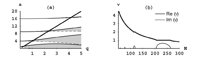
Figure 11: (a) Stability diagram for the Mathieu’s functions in a vs. q space. Unstable regions are shaded. The dashed curves correspond to an integer value of $\nu$ for the odd Mathieu functions, $S$, and the solid curves to an integer value of $\nu$ for the even Mathieu functions, $C$. Also shown is the solid line plot of $a$ vs. $q$ for the frequency variation model of Eq. 114 when $T=100$ ($\approx 120\cdot 2\pi/\omega_{0}$) $\mu$s; $g=0.5$, $\omega_{0}/2\pi=1.173$ MHz, for $50<M<300.$ The largest value of $M$ corresponds to the point on the line closest to the origin. (b) Plot of the real (heavy line) and imaginary (light line) parts of the characteristic exponent $\nu$ as a function of $M$ for the frequency variation model of Eq. 114 when $T=100$ $\mu$s and $g=0.5$. The imaginary values have been scaled by a factor of 5 to make them more visible on the graph. The solutions of Mathieu’s equation are unstable when $\nu$ is complex, with integer real part. The range of values of $M$ corresponding to unstable solutions is larger for smaller values of the characteristic exponent.

First, let’s consider the case $M=0,$ which is appropriate for shuttling in a short step, so that the frequency of the shuttling potential is decreased and then increased back to its original value just once. Again, we’ll consider the step size to be $2.14$ $\mu$m, and the frequency of the trap at the beginning and end to be $\omega_{0}/2\pi=1.173$ MHz. Ignoring the impact of any inertial forcing, the contribution to the average final state of the shuttled ion from the frequency variation of the potential will therefore be a function of the shuttling time and the modulation depth $g$. For shuttling times much less than one trap oscillation period, the impact of frequency variation of this type on the motional ion state is negligible, as expected (Fig. 12). As the shuttling time increases above the oscillation period of the trap, the average final state of the ion reaches a maximum and then rapidly decreases to an asymptotic value for all values of the modulation depth, $g$. For shuttling times greater than roughly 5 trap oscillation periods, $\langle n\rangle$ no longer depends on the shuttling time and becomes a simple function of $g$, as seen in Fig. 12. In general, the impact of this type of perturbation on the ion’s final state is minimal for any reasonable frequency squared modulation depth, $g$ and shuttling time, $T$.

Figure 12: Figure (a) is a plot of the numerically calculated average motional state $\langle n\rangle$ of an ion versus the modulation depth $g$ of the trap frequency squared, with $M=0$, for shuttling times $T=1$ $\mu$s (—) and $T=5$ $\mu$s (- - -), respectively. The distance shuttled in each case is for 2.14 $\mu m$. Figure (b) is a plot of the numerically calculated average motional state $\langle n\rangle$ of an ion versus the shuttling time $T$ in microseconds, with $M=0$ and $g=0.5$.

The second case to be considered is for longer shuttling times and distances, with a series of rises and falls in the shuttling potential frequency. This model might represent the frequency variation a shuttled ion would experience as the ion passes through areas in the trap array where the trap depth is successively weaker then stronger due to periodic arrangement of the electrodes in the trap array. Even in the case where the shuttling potential is kept constant along the ion’s trajectory, frequency variations in the transverse trap potential may be occurring periodically, feeding energy into the transverse modes of the ion’s motion through a subharmonic resonance. It might also represent the fluctuations in the axial trap frequency resulting from fluctuating voltages on the control electrodes. We now consider a fixed shuttling time of 100 $\mu s$ over a distance of 400 $\mu$m. For these parameters, it was shown in Sec. 3.3.2 that a hyperbolic tangent shuttling potential minimum time profile with $N=4.5$ produces minimal inertial forcing on a Cd⁺ ion, and so we can focus on the impact of the frequency variation on the ion’s final motional state. As discussed above, the solutions for the parametric oscillator are stable or unstable, depending on the value of the characteristic exponent, $\nu$. Now, as can be seen from Eq. 116, for a particular amplitude of frequency variation given by the parameter $g$, the relationship between $a$ and $q$ for the shuttled ion will be fixed along a line in $a-q$ space given by $a=2q/g$ (Eq.  116). This curve is shown for the specific value $g=0.5$ in Fig. 11a by a heavy line. Smaller values of $M$ are to the right and up, and larger values of $M$ are to the left and down, corresponding to values of $a$ and $q$ located closer to the origin. If the amplitude $g$ of the variation were to increase from this value, then the slope of the line in Fig. 11 would decrease. It is then clear from the stability diagram in Fig. 11a that this line would pass through larger and larger sections of the unstable regions. Therefore as $g$ increases, the likelihood of an unstable solution will also increase, as expected.

From Eq. 116 we see that both dimensionless parameters $a$ and $q$ are proportional to the factor

$$T_{fv}=\left(\frac{\omega_{0}T}{(M+\frac{1}{2})\pi}\right).$$ (119)

Since $\omega_{0}T/2\pi$ is the duration of the shuttling protocol measured in periods of the ion’s secular motion, $T_{fv}$ is the ratio of the effective shuttling time to the number of cycles of frequency variation of the shuttling potential. Therefore, we call $T_{fv}$ the period of frequency modulation. If the beginning and ending frequencies of the shuttling potential are equal, $M$ is an integer. Therefore, the values of $a$ and $q$ for this model of parametric frequency modulation are not continuous functions of $T_{fv},$ but are discrete points along the line in Fig. 11 for a given value of $g$. Those points are relatively farther apart for small values of $M$, and closer for larger values of $M$, when $a$ and $q$ are both small. The relative spacing between points on the line is a function of the total shuttling time. For longer shuttling times, the points all along the line will be closer, and for shorter times, the points will be placed farther apart.

This has a significant impact on whether a given frequency variation will result in a catastrophic shuttling protocol. For example, the line drawn in Fig.11a corresponds to the values of $a$ and $q$ for a frequency variation of 50% over a time of $100$ $\mu$s $\approx 120(2\pi/\omega_{0}).$ The line passes through all four regions of instability drawn on the diagram. These regions correspond to integer values of the real part of $\nu$ from 1 to 4 as one moves away from the origin. The corresponding values of $T_{fv}$ are roughly 1, 2, 3 and 4. The range in $M$ for which the shuttled ion’s motion is catastrophically unstable grows markedly for higher values of $M$, corresponding to smaller values of $T_{fv}.$ This is partially accounted for by the fact that the extent of the regions of instability through which the line in Fig. 11a passes does shrink as one moves up and to the right along the line (corresponding to smaller values of $M$). This effect is enhanced by the fact that the spacing between successive values along the line is increasing in that direction as well. As a result, the range of values of $M$ for which the parametric driving is unstable grows significantly for increasing $M$. This is illustrated in Fig. 11b, where the imaginary part of $\nu$ is scaled by a factor of 5 to make evident which values of $M$ will result in unstable parametric oscillations. As seen in the figure, only one or two values of $M$ at 57 and 78 correspond to unstable solutions with the real part of $\nu=4$ or $3$, while 60 values of $M$ from 205 to 265 are unstable when the real part of $\nu=1.$ Since the regions of instability for a given value of $g$ are determined by the value of $T_{fv},$ a shuttling protocol that takes 10 times as long to complete would require 10 times the number of frequency variations to observe the same unstable behavior. But it would also expand the range of values of $M$ for which the solution is unstable by a factor 10.

We find that longer shuttling times can result in unstable behavior at larger values of $T_{fv}$, corresponding to slower rates of frequency variation, while none was observed for the shorter duration shuttling protocols. This points to a new potential source of ion heating and possible trap loss during shuttling: in the rest frame of the ion electric field inhomogeneities along the ion trajectory will appear as electric field noise [51, 52].

The impact of these instabilities on the average final motional state of a shuttled ion can be seen in Fig. 13a. They are indeed catastrophic. On the other hand, if $M$ is kept to values much smaller than the number of ion oscillations during the shuttling protocol, so that $T_{fv}\gg 3$, the solutions $X_{1}$ and $X_{2}$ generally remain stable, and the impact on $\langle n\rangle$ is quite small, even for the large modulations ($g=0.5$) in the shuttling potential frequency assumed for this calculation, as seen in Fig. 13b. Although resonances are predicted for all integer values of $T_{fv}$ , they become increasingly narrow and less significant at larger values. This is particularly true given the fact that the modulation of the frequency will not likely be exactly sinusoidal, and the resonances correspondingly dampened. Therefore, as a rule of thumb, we can say from the above analysis that a shuttling protocol that has fractional variations in the trap frequency squared of less than 20% ($g<0.2$) and a period of frequency variation much greater than one,($T_{fv}\gg 3$) typically will not perturb the motional state of the shuttled ion.

Figure 13: (a) Plot of the calculated average motional state $\langle n\rangle$ of an ion versus $M$ (given by the modulation frequency of the trap). The shuttling time is 100 $\mu s$ and the modulation depth is $g=0.5$. For $M>80$, resonances can be observed arising from unstable regions in the Mathieu a-q plane. (b) Plot $\langle n\rangle$ versus $M$, with $T=100\mu s$ and $g=0.5.$ For $M<70,$ corresponding to a period of frequency variation $T_{fv}>3.3,$ the impact on the final motional state of the ion is minimal.

4 Shuttling and trap design

In this section, we discuss the problem of shuttling atomic ions through junctions and in multiple dimensions. Shuttling in two dimensions is useful for the realization of simple quantum algorithms, and may also be indispensible for the implementation of quantum error correction [55]. By shuttling many atomic ion qubits simultaneously, error correction can be perfomed in a massively parallel fashion, thereby lowering the fault-tolerant error thresholds [56]. The ability to shuttle effectively is intertwined with the design of trap architectures. Linear shuttling has been previously implemented in a series of experiments employing extended linear rf traps [18, 21, 23, 57, 26, 59]. Multidimensional shuttling was accomplished in a T-junction, where the rf nodal trapping pathways of three linear traps are joined at the junction. In this trap, ions were shuttled between traps through the junction, and the positions of two ions were swapped by executing a “three point turn” through the junction [26].

Near a junction, the trapping potential is no longer strictly a linear trap. The ions may encounter large rf fields in this region. This gives rise to a repulsive ponderomotive axial force pushing the ions away from the junction. The additional static forces necessary to confine the ion in the presence of theses new axial rf forces can weaken or destabilize the trap, allowing the ions to escape. Therefore, care must be taken when designing the trap junctions so that sufficient confinement is maintained while ions are transferred from one pathway to another. In order to make our discussion of the nontrivial features of the rf ponderomotive potential near a junction more precise, we define three terms:

• An rf hole describes the occurrence of an unstable (non-trapping) region of the rf ponderomotive potential near a trap junction, typically out of the plane of the ion pathway (Fig. 14a).

• An rf barrier is a region of non-zero ponderomotive potential along the ion pathway as it approaches a junction (Fig. 14a,c).

• An rf hump is a displacement of the minimum of the ponderomotive potential in a direction perpendicular to two or more merging ion pathways (Fig. 14c)  .

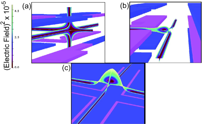
Figure 14: Plots of the rf pseudopotential for an asymmetric, cross-junction trap and two symmetric T-junction traps having two and three electrode layers, respectively. The electrodes are separated by 80 $\mu$m in the asymmetric trap, and 200 $\mu$m in the symmetric traps. The rf electrodes are shown in light pink, while the grounded layers are blue. In all three simulations, the rf voltage was set to 1.0 V. The contour plots are of the Electric Field amplitude squared, going from dark red to light yellow as the values range from 0 to $4.90\times 10^{5}\left(V/m\right)^{2}.$ Notice the rf barriers along the ion pathways for the asymmetric and three layer traps, while the two layer trap has an rf hole at its center. The rf hump in the pseudopotential for the asymmetric trap is also clearly seen.

These three features of the ponderomotive potential are illustrated in Fig. 14. The rf barrier, which occurs in all multidimensional junction traps explored to date, represents a region near the junction in which the rf ponderomotive potential impedes ion shuttling. An rf hole can occur in some trap geometries, and must be either avoided either by design, or the ions must be steered around the hole. An rf hump is typically present near junctions in asymmetric traps, described below.

4.1 Trap geometries

Trap designs that address the need for two-dimensional control of ions presently fall into two broad categories, symmetric and asymmetric traps, which are characterized by the degree of symmetry of the trap electrodes in the third dimension perpendicular to the plane in which the ion trajectory is confined. Both designs have advantages and disadvantages of their own related to issues of heating, and of electrical and optical access. The next sections compare these two geometries with special attention to multidimensional shuttling.

Symmetric ion traps feature rf electrodes that are located symmetrically around the ion pathway. Symmetric traps may be more difficult to fabricate because they typically require multiple layers, but they also feature high trap depths and efficient pushing forces on ions. Symmetric ion traps include two-layer traps, which have the rf electrodes arranged in two planes above and below the plane of the ion pathway [51, 57, 61], and three-layer traps, where the rf electrode is confined to a single layer in the plane of the ion pathway and two outer layers held at rf ground consisting of segmented electrodes that carry static voltages [62, 26].

Two-layer symmetric traps have drawbacks. Compensation of uncontrolled external static fields in three dimensions (potentially giving rise to large amounts of micromotion [35]) requires extra electrodes or the application of static voltages to the rf electrodes. More importantly, the junction region in two-layer traps is complicated by the fact that the rf electrodes are not in the same plane as the rf nodal pathways (See Fig. 14). This lack of lateral symmetry usually produces an rf hole at the junction center, and the ions must then be carefully steered around the hole and through sizable rf barriers for successful transit. A variation of the two-layer trap with small bridges extending diagonally across the junction has also been proposed to close that hole, at the cost of introducing rf barriers along the ion pathways [63].

Three-layer traps [62, 26] can have both vertical symmetry (perpendicular to the multiple channels forming a junction) and transverse symmetry, and allow for complete three-dimensional compensation of background static fields exclusively through the control electrodes. Shuttling through a junction is also simpler in three-layer traps, as the added symmetry avoids rf holes at the junction.

Asymmetric traps, also referred to as single-layer traps or surface traps, have all their electrodes located in one or more planes below the ion pathway [64, 65, 66]. This offers clear advantages in the context of large-scale fabrication, as the electrical lead-ins can be fed from the underside of the trap electrode surface, at the expense of more restricted optical access.

It is possible to greatly reduce the effect of the rf barrier in both the symmetric and asymmetric trap junctions by tapering the (surface) electrodes in the approach to the junction [67]. This serves to increase the size of the region along the ion pathway in the linear portion of the trap having a non-zero axial electric field component and effectively spreads out the rf barrier that the ion must pass through. While the total work necessary to transport the ion through the junction would not change, the force required to advance the ion at any point along the pathway can be significantly reduced. For the asymmetric trap this also reduces the characteristic trap size near the junction and pushes the ponderomotive minimum closer to the trap surface, minimizing the rf hump. However, the rf barrier also effectively reduces the depth of the trap over the range of its spatial extent, which could be an issue for shallow traps.

4.2 Shuttling through junctions

Shuttling through junctions, where three or more linear trap axes join, is greatly complicated by the presence of rf barriers leading into the junction. These barriers can result in added kinetic energy to the ions that is dificult to control, and in some cases loss of the ion from the trap altogether. The increasing complexity of the trap design and the greater demands on precise knowledge of the trap fields means that accurate numerical simulation of the fields as outlined earlier in this paper becomes essential.

Although rf barriers are present in all trap junctions considered here, we will examine their influence and characterize their features in a simple, three-layer T-trap. The spatial extent of these rf barriers and the potential gradient along each side of the barrier determine how the ion can be reliably carried through the junction. For the ion to make it through the barrier in a controlled fashion, the potential energy gradient of the guiding control fields should be at least as great (and opposite in sign) as the gradient in the rf pseudopotential barrier. Otherwise, the ions must be given enough kinetic energy to make it through. If the gradient is canceled only on one side of the barrier, the ions will still be accelerated by the gradient in the rf ponderomotive potential as the ion enters the junction, again giving the ions unwanted kinetic energy. Thus it is most desirable to reverse the sign of the potential energy gradient on both sides of the barrier, so that the ion remains in a smooth axial trap throughout its motion. This suggests a strong relationship between the spatial extent of the rf axial barrier, and the maximum size of the control electrodes used to shuttle the ions. Tapered electrodes at the junction serve to relax this maximum size restriction. The strength of the rf barrier is also related to the trap depth perpendicular to the plane of the ions’ motion at the junction, and if the quasistatic control forces are too high, then they will destablize the trap out of the plane of the junction. In sum, the four most important features of the rf barriers are their spatial extent, gradient, strength and the trap depth out of the plane at the barrier location.

As dimensional analysis suggests and numerical simulations show, all of these features are controlled by the characteristic distances of the trap architecture near the junction. These include the channel width of the trap, $a$, defined by the perpendicular distance between the rf electrodes and the rf nodal pathway, the aspect ratio of the trap, $\alpha$, defined by the ratio of the channel width, $a$, with the vertical separation, $d$, between the rf and control electrodes, and finally, the ratio, $\delta$, which is defined by the distance between the electrodes, $h$, to the thickness of the electrodes, $w$. This last ratio is significant only in the case of very large aspect ratios. The salient features of the rf barrier for most traps are set primarily by the channel width $a$. The rf barrier results from unbalanced fields produced by the electrodes across the junction, as well as from the corners of the nearest electrodes. Therefore, as a practical matter, it is best to design the trap so that the control electrodes are segmented into pieces having a width less than or equal to $a$. This guarantees that quasistatic control field gradients can be generated to overcome the rf barrier gradient. This simple rule of thumb was shown in numerical simulations to be sufficient to reliably shuttle the ions around the corner of both two and three layer traps. If the control electrode segments are much larger than $a$ (such as in the T-junction array of Ref. [26]), the shuttling procedure involves control electrodes that are far removed from the ion’s position, and very high voltages are required to produce static potential gradients that cancel those of the rf barrier. Such a protocol may result in the ion acquiring a significant amount of kinetic energy that will need to be mitigated via laser cooling, sympathetic cooling, or phase sensitive switching of the trapping potentials.

The rf barrier strength for a three layer trap of width $a=100$ $\mu$m and electrode thickness $w=20$ $\mu$m is shown for various trap aspect ratios $\alpha$ in Fig. 15.

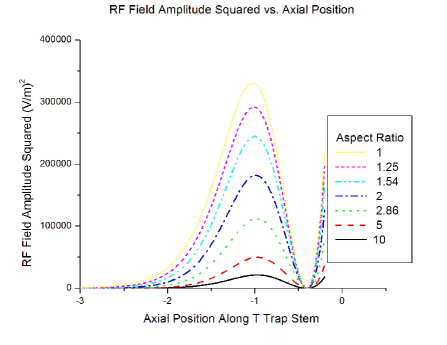
Figure 15: A plot of the rf electric field amplitude squared vs. axial position along the axis of the stem of a three layer T trap with one volt applied to the rf electrodes. The axial position is scaled with the channel width, $a=100\mu m$. The origin is at the center of the T-junction. The electrode thickness was modeled to be $d=20\mu m$, and aspect ratios, defined as the ratio of the distance from rf electrode tip to rf electrode tip to the distance between the rf electrodes and the control electrodes (see Fig. 17), $\alpha$, were chosen ranging from 1 to 10.

Note that the spatial extent of the barrier is largely unaffected by aspect ratio. However, the barrier strength decreases dramatically as the aspect ratio increases, as the figure illustrates. This can be understood by considering the effect of the control electrodes as they come closer to the rf electrodes, drawing the electric field lines from rf to control electrodes and reducing the electric field amplitude uniformly out in the channel. Aspect ratio also has a direct impact on trap depth (Fig. 16 (b)), so that trap depth increases with decreasing aspect ratio, up to the limit of an aspect ratio of $\approx$ 1/2. Below that limit, the geometry approaches the situation of an rf layer with ground at infinity, and the depth therefore begins to drop again to its asymptotic value. By taking the ratio of rf trap depth to barrier strength, we obtain Fig. 17. This figure shows that the trap depth remains at least ten times as great as the barrier strength, even for large aspect ratios, while it increases to twenty five for an aspect ratio of 0.25. By decreasing the trap aspect ratio in three layer junctions, the trap depth at the junction can be made much larger than the rf barrier strength, providing a large margin of safety for reliably shuttling through the junction. More importantly, by increasing the aspect ratio of a three-layer junction, the rf barrier can be made arbitrarily small while retaining a strong trapping potential inside the junction region.

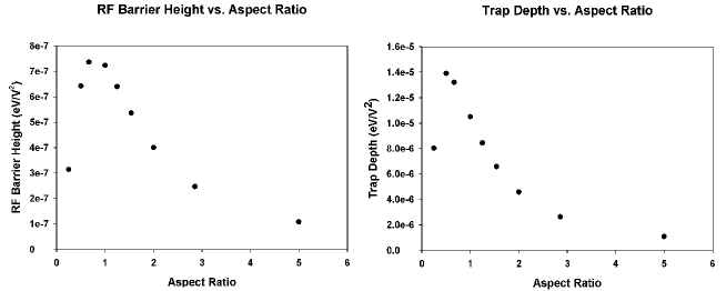
Figure 16: Plot of the rf barrier strength and trap depth at the barrier maximum versus the aspect ratio in a three layer symmetric T-trap array with 1 volt applied rf. The aspect ratio is defined to be the ratio of the rf layer channel width to the tip to tip separation of the rf and control electrode layers. It is possible to decrease the rf barrier height at the expense of trap depth by increasing the trap aspect ratio.

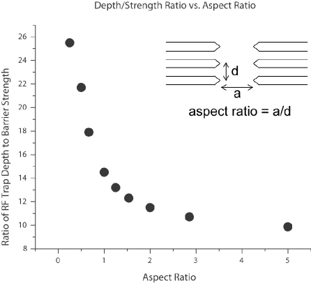
Figure 17: A plot of the ratio of rf trap depth and barrier strength vs. aspect ratio in a three layer T trap. The T has channel width $a=100\mu m$ and electrode thickness $d=20\mu m$.

5 Practical implementation of shuttling operations

5.1 Introduction

In order to realize most quantum computing architectures with trapped ions, it may be necessary to shuttle ions between memory (storage) zones and interaction (entanglement) zones. To bring any two ions together in an entangling zone, it is necessary to be able to sort a linear chain of ions into any desired order. This requires the successful implementation of four key protocols: separating two ions that are located in the same trap, linearly shuttling two ions that are in the same trap, recombining two ions together into one trap, and shuttling ions around corners through a junction on an individual basis [18, 21, 23, 57, 26]. The combination of all four elementary protocols allows for arbitrary control of trapped ions in two dimensions.

The simulation of ion trap potentials via the method of basis functions has thus far been completely general. The power of this method and its utility for simulating potentials will be shown by analyzing the shuttling protocols used in experiments at the University of Michigan [26] where ions are shuttled linearly, around a corner, and are swapped in an 11-zone, three layer T-junction ion trap array (see Fig. 18). Discussing the practical implementation of shuttling operations in this particular geometry will serve as an instructive example and will provide recipes to develop shuttling protocols for arbitrary geometries. As discussed in Sec. 4, there are ways to design optimal ion trap geometries. However, fabrication constraints (such as the longitudinal extension of the corner electrode inside a junction) may result in non-optimal trap geometries. The strategies that will be introduced in order to overcome such constraints for the T-junction array discussed here are therefore of general interest for designing shuttling protocols in any two-dimensional ion trap.

The Michigan T-junction ion trap array [26] has 49 electrodes and a sufficient number of trapping zones to swap the positions of two ions. The central layer contains a T-shaped channel; the electrode is formed by depositing gold around the channel with an electron beam evaporator on an alumina substrate. Gold-coating of the 24 control electrodes on each of the two outer layers is accomplished with dry-film photolithography and wet-chemical etching. Here, electrodes and tracks are formed by depositing 0.015 $\mu$m of titanium followed by 0.4 $\mu$m of gold. Two thin alumina spacer plates are inserted between each outer layer and the central rf layer substrate. All three substrates are held together via rectangular alumina mount bars. Chip capacitors and resistors are ribbon-bonded onto a gold coated quartz plate that is mounted adjacent to the alumina substrates (top and bottom of figure 19). To isolate the control electrodes from external noise and from induced rf from the nearby rf electrode, each of the 28 non-grounded control electrodes is immediately shunted to ground via a 1 nF capacitor and then connected in series to a 1 k$\Omega$ resistor leading to the vacuum feedthrough.

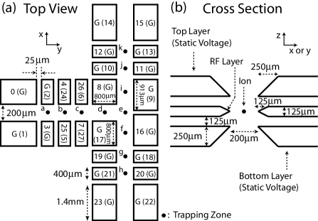
Figure 18: Top view and cross section of the Michigan T-junction ion trap array showing all 11 trapping zones a-k [26]. The control electrodes are numbered with bottom-layer control electrodes in parentheses. G indicates a grounded control electrode.

The trap array has a plane of symmetry along the $xy$ plane through the rf layer, and a second in the $yz$ plane which divides the trap along the stem of the T, with the origin at the center of the junction of the T. The trap array was modeled in Vector Fields’ Opera by centering it in a bounding box extending 20,000 $\mu$m in all three directions. For simulations done on an Intel 4, 2.8 GHz processor with 1.0 GB of RAM running Windows XP, the number of nodes in the problem ranged from 1 to 2 million. When calculations for the rf pseudopotential were carried out, the node spacing was made tightest in the junction region of the T, where it reached a minimum of 10 by 10 by 1.5 $\mu$m. When calculations for the control electrode basis functions were performed, the node spacing was kept at 10 by 10 by 3.0 $\mu$m along the electrodes where the potential changed most rapidly. The electrodes themselves were excluded from the simulation volume.

The rf pseudopotential used to trap ions in the T depends on the square of the electric field amplitude produced when the rf layer is at the maximum voltage and the two outer layers of electrodes are held at rf ground. To estimate the error in the calculated electric field, a comparison was made between the simulation used to determine the rf pseudopotential, and an identical model with the mesh density doubled throughout. (Because of memory limitations, this higher mesh density model took one month to run on a 3.2 GHz dual-processor PC workstation with 1.0 GB of RAM, running Windows XP.) The voltage used on the rf layer in both cases was 1.0 V. The field was evaluated for both models along a grid of points along the entire length of the top channel of the T, and the fractional difference in the field was evaluated at each point. The average fractional difference was equivalent to a 0.15% error. This average was sharply skewed upward because of the presence of the nodal lines along the center of channel due to field cancelation. Along that line, fractional errors of 60% were reached. The difference in actual values of the field along the nodal line, however, corresponded to less than 1 V/m. This is insignificant when compared to the fields of thousands of V/m just microns off axis. The electrostatic potential calculations done with the same mesh spacing had significantly smaller errors than even these. Once these fields have been determined numerically, it becomes possible to construct the basis functions necessary to calculate and analyze the required shuttling protocols.

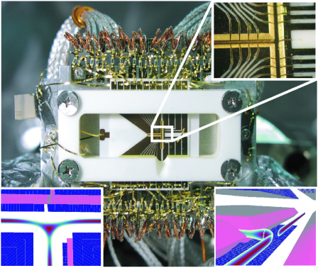
Figure 19: T-junction ion trap with associated RC filters, wirebonds, and wires. The T-junction ion trap is an eleven zone ion trap with 48 DC electrodes of which 28 are connected to variable external voltages. The fabrication of the ion trap array required over 500 wire bonds. The inset in the upper right corner shows a magnified view of the junction region. The segmented linear DC control electrodes have an axial extent of 400$\mu$m while the corner electrodes have an axial extent of $\sim$800$\mu$m. The graph in the lower left is a plot of the rf pseudopotential near the T-junction and shows the RF barriers that impede entry to the junction region from all three directions. The picture in the lower right is a perspective view of the potential looking down the channel in the top of the T-junction.

5.2 Linear Shuttling

The most elementary shuttling protocol is moving an ion along a linear path from one position to another. In a segmented linear rf Paul trap, this procedure implies shuttling the ion along the rf node between trapping zones. Several notable experiments have already utilized linear shuttling protocols, and have demonstrated essentially unit probability of success [18, 57]. Here we describe the design and the implementation of a shuttling protocol for linear ion transport that holds the secular frequency constant. This constraint allows us to use the simplified analysis of section 3.3.1.

The simulations of trap voltages via the basis functions described in Sec. 2.3 allow us to determine both the trap frequencies and the position of the trap. The design of the shuttling protocol begins by determining the start and end locations of the trap; for instance, zones c (start) and b (end) in Fig. 18. The total shuttling distance may then be broken up into any number of steps, where the finite time needed to change the voltages on the electrodes establishes an upper bound for the total steps required. The frequency of the potential should be kept constant throughout this process. In order to determine the voltage changes required for each step in the experiment, two actions are undertaken in the numerical simulations. The first is to iteratively adjust/produce an asymmetry between the electrodes serving as the endcaps of the current trapping zone, thereby moving the minimum of the potential in the axial direction by the designated amount (to within some arbitrary choice of error). The change in voltage will usually alter the axial trap frequency as well. The second action seeks to compensate for this by multiplying all the voltages by some scale factor, iteratively adjusted until the previous secular frequency is once again obtained. While multiplication by this scale factor appears to have negligible effect on the position of the potential minimum, any shift could always be accounted for by iteratively repeating these two previous actions. This method is very robust in that each step is some small shuttling distance, which may be used to produce any time dependent behavior (e.g. linear, sinusoidal, or transcendental potential minimum time profile) for the potential minimum, $x_{0}(t)$, in the total shuttling protocol as described in Sec. 3.1. The final product is an array of voltages in which the axial trap frequency is kept nearly constant  .

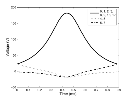
Figure 20: This shows the voltages on the various electrodes of the trap while the ion is linearly shuttled from zone c to b.

Using the scheme described above, we generated a shuttling protocol consisting of 200 discrete time steps that shuttled the ion from zone c to b, a distance of $425$ $\mu$m in $1$ ms. The ion was moved a constant distance at each step, $2.14$ $\mu$m, resulting in a linear potential minimum time profile. The axial trap frequency was kept at 1.173 MHz with a tolerance of 0.5%. The voltage sequence is shown in Fig. 20. The experiment was carried out such that a single $\mbox{Cd}^{+}$ ion was laser-cooled, shuttled, detected, and then laser-cooled once again. The success rate was observed to be $>99.999$% (100000 attempts). Hence, we have demonstrated a linear shuttling protocol that has virtually unit probability of success.

In order to show that the shuttling protocol is adiabatic, it is necessary to cool the ion to the ground state and measure its temperature before and after the shuttling operation. A somewhat weaker test would be to shuttle the ion back and forth many times between two trapping zones without the application of any laser cooling. If the boil-out time (the time it takes for the ion to be heated out of the trap) remains unchanged with and without the shuttling operation, weak evidence for adiabaticity is obtained. This test would constitute a necessary but insufficient condition for the shuttling process to be adiabatic.

5.3 Corner Shuttling

5.3.1 General considerations

There are many challenges associated with shuttling an ion around a corner. First of all, a suitable control electrode geometry should be chosen to give maximum control over the ion in the junction region. Specifically, the control electrode widths should be no larger than the channel width of the ion trap array. It is still possible to shuttle ions around a corner using electrode sizes that are larger than the channel width [26], but it becomes difficult to control the motion of an ion in the junction region. Smaller control electrodes also make it easier to overwrite rf barriers near junction regions without destabilizing the trap in the transverse direction, however practical fabrication and operation constraints will typically place certain limitations on the electrode geometry. In addition for the case of asymmetric (planar ion traps) one also needs to account for the presence of rf humps (see Sec. 4).

Secondly, large electrodes near a junction region can make it difficult to maintain constant trap frequencies when shuttling an ion into a junction region without destabilizing the trap in the transverse direction. Maintaining constant trap frequencies may be an important factor in minimizing acquired kinetic energy when shuttling ions around a corner as is discussed in Section 3.3. This presents a unique challenge when shuttling an ion around a corner because the weak axis of the trap rotates. For example, when shuttling from zone d to zone i (see Fig. 18), the weak axis is originally in the y-direction when an ion is in zone d. After an ion is shuttled around the corner to zone i, the weak axis is in the x-direction. Smaller control electrodes should help maintain a constant trap frequency along the weak axis.

A third challenge to corner shuttling which may arise is the accurate simulation of an ion’s motion through an ion trap array. The advantages of the Bulirsch-Stoer method are discussed in Section 2.4 and the Appendix. The accurate simulation of an ion’s classical motion plays a key role in calculating the average motional state of the ion during shuttling. A limitation to the accuracy of numerical solutions of an ion’s trajectory can arise in the form of a local maximum in the plane of the trap array when trying to overwrite the rf barrier. For example, in the T-trap, there is a small local maximum in the pseudopotential at $t=25$ $\mu$s in the xy plane during corner shuttling near the center of the junction near zone e (see Fig. 18) that slopes down toward zone i and zone f. A local maximum in the pseudopotential means that the calculated motion is sensitive to perturbations in the initial conditions or phase of oscillation of an ion and can cause errors in an ion’s calculated trajectory in the junction region. The issue of having a local pseudopotential maximum is related to control electrode size; smaller control electrodes should allow a control electrode potential to overwrite any small local potential maximum.

Another issue important to the accuracy of the numerical simulation is whether to use the pseudopotential approximation when simulating the rf trapping field. As was discussed earlier, it is possible to simulate the ion’s motion either with the time averaged pseudopotential (Eq. 16) or the actual rf potential (Eq. 15). In any of the junction geometries considered in this paper, it is impossible to maintain an ion near an rf node throughout a corner shuttling procedure, making the impact of micromotion on the ion trajectory potentially significant. In addition, if the shuttled ion does pick up a significant amount of kinetic energy, it will likely explore regions in the final trapping configuration where micromotion is potentially large. In our case study of the T-junction array, the ion typically picks up  0.5 eV of energy due to micromotion alone. This is comparable to the final kinetic energy of the large scale secular motion of the ion. Therefore, despite the computational speed-up (in our case, a factor of 2) by using the pseudo-potential, in order to fully understand the ion’s motion through a junction, one should simulate the ion’s motion using the sinusoidally varying rf potential from Eq. 15 if there is any uncertainty whether the process is fully adiabatic.

In order to provide a detailed overview on how such a corner shuttling operation is achieved, we discuss the particular example of shuttling an ion around the corner inside a T-junction ion trap array [26]. This particular array is limited by the fact that the control electrodes at the corners of the junction are too large (4 times larger than the channel width) to achieve adiabatic shuttling throughout the junction. In contrast, the ions in this trap are pushed through the rf barriers by applying very high control electrode voltages on those electrodes (labeled 6, 7, 26, 27, 10, 11, 18 and 19 in Fig. 18) that are nearest neighbors to the corner electrodes of the T. These large, but distant, voltages produce a sufficiently positive gradient in the potential at the position of the rf barriers so that the ions can be pushed into the junction region and then directed through one of the rf barriers in the top of the T to be trapped in one of the zones labeled f through k. In doing so, an ion gains $\approx$1 eV of kinetic energy. The large extent of the corner electrodes and the finite trap depth in the junction of the T means that performing detailed numerical simulations was crucial for determining those shuttling protocols which would successfully move ions through the junction of the trap array. Constraints in future trap designs is likely to remain significant as the demands on the performance of these traps increase as well. An ion trap array that contains many qubits may require many thousands of electrodes to carry out any needed shuttling operations. It is inevitable that fabrication constraints may result in non-optimal geometries. Therefore, the numerical analysis of the T-junction ion trap array [26] and the comparison of the simulated ion dynamics with experiment during the operation of this trap provide a good case study when considering the process for scaling up current trap technology to meet the demands of quantum information processors and other ion trap applications.

5.3.2 Stem-to-top corner shuttling in a T-junction array

Here we describe the process of stem-to-top corner shuttling using the specific example of a T-junction ion trap array [26]. An ion is initially trapped in zone d (see Fig. 18) with trap frequencies ($\omega_{x}/2\pi$, $\omega_{y}/2\pi$, $\omega_{z}/2\pi$) = (5.0 MHz, 0.7 MHz, 4.9 MHz). Figure 21 shows the voltage time profile used to shuttle an ion around the corner.

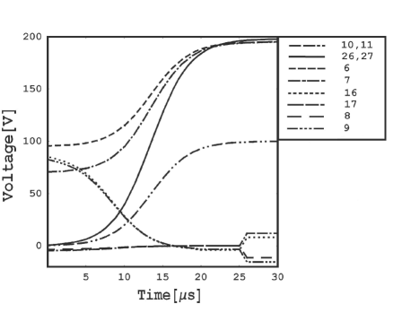
Figure 21: The control electrode voltage profile for the corner shuttling protocol. The figure shows the voltages applied to the relevant electrodes to execute the corner shuttling protocol.

The voltages of control electrodes 6, 7, 26, 27 are raised to $\sim$200 V in $\sim$ 20 $\mu$s using hyperbolic tangent voltage vs. time profiles to push the ion toward the junction region. Note that this voltage time profile does not imply that the potential minimum of the trap follows a hyperbolic tangent in time (see Eq. 27). It is possible to specify a particular potential minimum versus time profile [58]. Simultaneously, the voltages of control electrodes 8 and 17 are raised from approximately -4 V to 0 V while control electrodes 9 and 16 are lowered from $\sim$80 V to -3 V. The net effect of these voltage changes over the first $\sim$ 20 $\mu$s is to push the ion through the rf potential energy barrier.

After going through the rf barrier, the ion is accelerated by the potential gradient on the backside of the rf barrier from $y=-220$ $\mu$m to $y=0$ $\mu$m in $\sim 2$ $\mu$s, acquiring $\sim$0.5 eV of kinetic energy in the process (see Fig 22 - 24). The ion continues in the y-direction past zone e toward the rf layer in the top of the T trap. The ion is pushed back by the rf potential toward zone e. Thus, the first step in the corner-shuttling protocol is to successfully move an ion into the junction region and then keep it trapped there until the next stage of the protocol is implemented. This is made difficult by the relatively weak trap in the junction region, and the ion’s relatively large kinetic energy acquired during its traversal of the rf barrier into the junction. Note that in the shuttling protocol as recorded in Fig. 21, the voltages on the control electrodes 8, 17, 9 and 16 all converge nearly to ground while the ion was in the junction region. High voltages on these electrodes can easily make zone e anti-trapping. There was a delicate tradeoff when designing the corner shuttling protocol for this trap. A sufficiently high potential gradient needed to be applied to push the ion through the rf barrier. At the same time, the control electrode voltages near the junction region needed to be kept near ground to prevent the junction region from becoming anti-trapping. The key to successfully shuttling an ion around the corner through the junction region proved to be finding the right balance between these two requirements.

When the ion is in the junction region, the four corner electrodes are used to guide the ion towards zone i. When the ion has reached the desired final trapping position at zone i, the control electrode voltages change to their final values in $\simeq 1$ $\mu$s. This rapid change in voltage is timed so that the ion crosses the final trap minimum as the voltages ramp up. Changing the voltages in this way helps to minimize any further contribution to the ion’s kinetic energy. Specifically, the voltages of control electrodes 16 and 17 are ramped to approximately $+10$ V while the electrodes 8 and 9 are lowered to approximately -10 V in 1 $\mu$s, “catching” the ion in zone i. Simulations incorporating micromotion show that the amount of kinetic energy added in this step is still considerable: 0.7 eV (see fig 23). The final trap position in zone i is defined by these voltages, with the resulting secular frequencies ($\omega_{x}$, $\omega_{y}$, $\omega_{z}$) = (0.5 MHz, 5.5 MHz, 4.3 MHz).

When the ion enters zone e, there is a local potential maximum in zone e. This local maximum places a limitation on the accuracy of numerical solutions because small perturbations in the initial position of the ion can cause the ion to go in radically different directions in the junction region. The optimization of the “catch” step described in the preceding paragraph is to ensure that when an ion does go past the potential maximum in the correct direction, the ion will be caught with little added kinetic energy. However, if the ion is guided by the local maximum toward the opposite direction, then the ion will gain considerably more kinetic energy as the voltages suddenly ramp up to form the final trap. In addition, there is some evidence that this is an effect that can be seen experimentally. Occasionally the ion was observed to crystallize in zone i one full second after being shuttled from zone d, a crystallization time several orders of magnitude longer than the crystallization time after linear shuttling. This could be due to the fact that the ion occasionally makes an excursion toward zone f which means that when the voltages suddenly change, the ion gains a lot more kinetic energy and takes longer to cool.

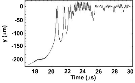
Figure 22: Simulation (including micromotion) of the ion’s position along the y-axis (axis of the stem of the T) in and around the junction region during corner turning. Note the accentuated micro-motion from $t=18$ $\mu$s to $t=20$ $\mu$s as the ion traverses the rf barrier.

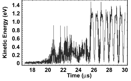
Figure 23: Simulation of the ion kinetic energy in and around the junction region during the corner turning protocol. Note the rise in kinetic energy after the ion crosses the rf barrier at $18$ $\mu$s and the abrupt rise in energy at the $25$ $\mu$s when the “catch” step is implemented.

The corner shuttling protocol was used to shuttle the ion from zone d to zone i in the T-trap in 26 $\mu$s with a success rate of greater than $99\%$ (881 out of 882 attempts) [26]. The speed of the shuttling protocol was limited by the RC filters and the speed of the analog output cards that supply voltage to high speed op amps that are connected to the trap electrodes.

Despite the high success rate of the shuttling protocol from zone d to zone i, we were unsuccessful in shuttling the ion from zone d to zone f using a voltage protocol mirrored at the y-z plane through the center of the stem of the T. This discrepancy may be attributed to static bias fields or a misalignment observed in the three electrode layers due to the manual assembly process. The use of semi-conductor etching techniques to build multi-layer ion trap arrays is one way to avoid such misalignments and asymmetries in the trap [59, 60]. Instead, a composite shuttling protocol was used. The protocol begins with shuttling the ion from zone d to i as described above, the ion is laser cooled and then shuttled from zone i to f in a linear fashion. The shuttling from i to f is not optimized to maintain constant secular frequency, however, the success rate was 100% (50 attempts).

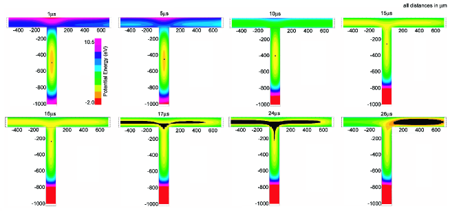
Figure 24: Potential energy map (in the pseudopotential approximation) as an ion is shuttled around a corner of the T-junction. The region energetically accessible to the ion is indicated in black. The kinetic energy of the ion is initially small, so the region of the T that the ion can energetically traverse is small. As the ion goes through the rf barrier, it acquires $\sim$1 eV of energy, so the region that the ion can energetically traverse is much larger.

5.3.3 Top-to-stem corner shuttling in a T-junction array

The shuttling sequence from trapping zone i to trapping zone d is similar to the shuttling protocol from zones d to i in that the ion must be pushed through the rf barrier without causing the trap to become destabilized in the transverse direction while the ion is in the junction region. However, there is an important difference between the two protocols in the T-junction trap array. In general, it is not possible to simply reflect the voltage profile that shuttled an ion from stem-to-top (zone d to i) in time in order to shuttle from top-to-stem (zone i to d). While Newton’s equations of motion are time-symmetric, the initial conditions of an ion being shuttled from zone i (for example after laser cooling) to zone d are not the same as the final conditions of the ion after it has acquired $\sim$1 eV of kinetic energy after being shuttled from zone d to zone i. Therefore, to use the time reflected stem-to-top control voltage profile in order to shuttle from top-to-stem, one would need to prepare the ion in zone i with initial conditions equal to the final conditions after the shuttling operation from d to i. The complexity of the geometry will determine how well the two sets of conditions will need to be matched. As this may be difficult to achieve one may have to design a new voltage control sequence. Per definition an adiabatic shuttling protocol can always be time reflected for a successful reverse shuttling operation.

Even though simply reversing the stem-to-top protocol was unsuccessful, it served as the basis for developing a working routine. In order to realize the top-to-stem protocol, the roles of the following electrodes are swapped:

$$9 \leftrightarrow 17$$ (120)

$$10 \leftrightarrow 6$$

$$11 \leftrightarrow 7$$

while electrodes 8 and 16 keep the same time dependent voltage profile. The successful shuttling protocol from zone i to zone d [26] starts with an ion in zone i with trap frequencies ($\omega_{x}$, $\omega_{y}$, $\omega_{z}$) = (0.7 MHz, 4.5 MHz, 4.2 MHz). The voltages on control electrodes 10 and 11 are changed to 200 V via a hyperbolic tangent function while simultaneously raising the voltages on control electrodes 8 and 9 from $-4$ V to ground and lowering the voltages on electrodes 16 and 17 from $35$ V to $-4$ V. This provides enough potential gradient to push the ion through the rf barrier into the junction region (zone e). Again, the ion gains $\sim$1 eV of kinetic energy after going through the rf barrier, and once the ion is in the junction region, it makes large oscillations in the relatively flat trap of zone e. Then the voltages on the control electrodes are suddenly ramped, as can be seen in Fig. 25, to form a trap in zone d with ($\omega_{x}$, $\omega_{y}$, $\omega_{z}$) = (5.0 MHz, 0.6 MHz, 3.6 MHz). The timing of this step is done in an attempt to have the voltage ramp occur when the ion is near the potential minimum to minimize the amount of kinetic energy gained.

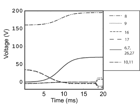
Figure 25: Control electrode time profile for corner shuttling from the top of the T to the stem of the T. A plot of the voltage vs. time for the electrodes used to shuttle the ion from the top of the T to the stem of the T.

The control voltage scheme in Fig. 25 successfully shuttled an ion from zone i back to zone d in the T-junction ion trap with a success rate of 98% [26] (118 attempts) with a total shuttling time of $30$ ms. The reliability of the shuttling protocol drops off dramatically if we increase the shuttling speed. We failed to observe any instance of successful shuttling if the shuttle time was less than 20 ms; this is 3 orders of magnitude slower than the shuttling scheme between zone d to zone i. If misalignments in the trap electrodes and stray electric fields are incorporated into simulations, one should be able to optimize the voltage control scheme so that an ion may be shuttled successfully from zone i to zone d just as fast as an ion may be shuttled from zone d to zone i.

5.3.4 Characterization and optimization of corner shuttling protocols

Once a shuttling protocol is created that successfully transports a single ion around a corner inside an array, a number of steps can be carried out in order to optimize the original shuttling protocol depicted in Fig. 21. Indicators for the quality of the protocol consist of the success rate of the protocol and estimations of the kinetic energy the ion acquires during the shuttling process based on numerical analysis. The corner shuttling protocols being discussed here can be refined using numerical simulations in which the relevant voltages on the corner electrodes are systematically perturbed. In order to illustrate this process we give a detailed discussion of such refinements that were carried out for the forward shuttling protocol used in the T-junction array [26].

The process of shuttling ions around the corners of the T-trap depended most sensitively on the voltages applied to the four junction control electrodes (electrodes 8, 9, 16, and 17) of the T-trap. The figure of merit to optimize in a corner shuttling protocol is the acquired kinetic energy during shuttling. In this case, the protocol was perturbed by changing the final electrode voltages of the corner electrodes before the sudden ramp in the voltages that defines the final trap in zone i as seen in Fig. 26. We define V${}_{i,j}(t)$ to be the time dependent voltage of the i-th electrode, where j is the target voltage for the electrode just before the sudden ramp at t= 25 $\mu$s (see Fig. 26). The simulations were examined to determine which set of voltages produced a successful shuttling operation, and gave the smallest gain in kinetic energy to the ion.

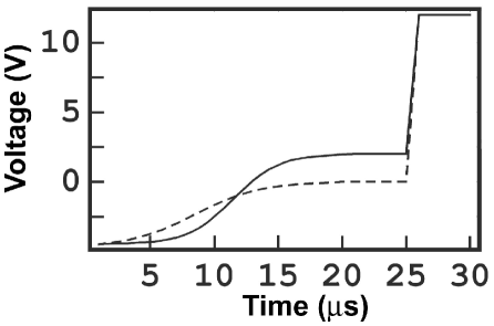
Figure 26: Example of the perturbation of the corner shuttling protocols. A time profile of the voltage on electrode 17 from the original forward shuttling protocol (dashed line) and the perturbation $V_{17,+2}$(t) (solid line) to that profile.

It is also important to consider the different ways a shuttling protocol might fail. There are three basic ways in which shuttling from zone d to zone i can fail. The ion might not make it through the rf barrier and becomes stuck in the original trapping zone. Alternatively, the ion could be ejected from the junction region because the trap becomes too weak in the z-direction. Finally, the ion could go too far toward zone f so that when the final voltage ramp occurs, the ion is ejected in the negative x-direction. Therefore, we examined the effect of the various perturbations on the control electrode voltages by simulating the shuttling process and recording the success or failure of the operation. The success was further characterized by the gain in kinetic energy, while the failure was characterized by the mode of failure observed. The results of this analysis are shown in the various stability plots in Figs. 27 - 30. Each plot show the reciprocal kinetic energy gained by the ion as a function of the target voltage on the corner electrodes. Unsuccessful operations are arbitrarily plotted with a reciprocal kinetic energy of 0 eV^-1 with the type of failure marked.

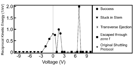
Figure 27: Stability plot for electrode 8. The plot shows the reciprocal kinetic energy gained by the ion as a function of the target voltage (as defined in Fig. 26) on electrode 8. The vertical line highlights the original protocol shown in Fig. 21. All failed shuttling operations are arbitrarily plotted with 0 reciprocal kinetic energy.

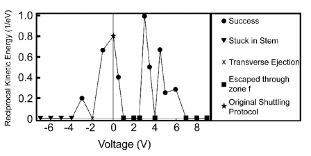
Figure 28: Stability plot for electrode 17. The plot shows the reciprocal kinetic energy gained by the ion as a function of the target voltage (as defined in Fig. 26) on electrode 17. The vertical line highlights the original protocol shown in Fig. 21. All failed shuttling operations are arbitrarily plotted with 0 reciprocal kinetic energy.

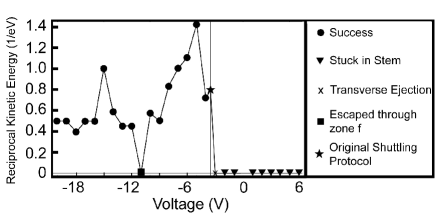
Figure 29: Stability plot for electrode 9. The plot shows the reciprocal kinetic energy gained by the ion as a function of the target voltage (as defined in Fig. 26) on electrode 9. The vertical line highlights the original protocol shown in Fig. 21. All failed shuttling operations are arbitrarily plotted with 0 reciprocal kinetic energy.

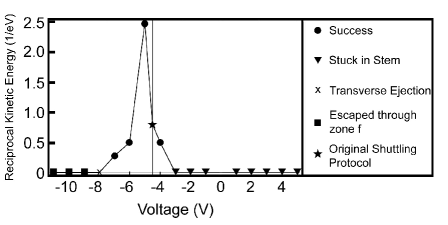
Figure 30: Stability plot for electrode 16. The plot shows the reciprocal kinetic energy gained by the ion as a function of the target voltage (as defined in Fig. 26) on electrode 16. The vertical line highlights the original protocol shown in Fig. 21. All failed shuttling operations are arbitrarily plotted with 0 reciprocal kinetic energy.

The corner shuttling stability plots show that there is a cutoff voltage lower than which the ion does not move out of the stem of the T-junction, but remains stuck near zone d. By not raising the voltages on control electrodes 8 and 17 high enough (Fig. 27, 28), the control electrodes cannot provide enough of a potential gradient to push the ion through the rf barrier. Similarly, by raising the voltages on control electrodes 9 and 16 too high (Fig. 30, 29), the shuttling sequences also fail. Perturbing the voltage on control electrode 9 by a large amount compared to the other three corner electrodes will still successfully shuttle an ion around the corner from zone d to zone i. By lowering the target voltage on electrode 9 before the sudden voltage ramp, the control electrode strongly attracts the ion toward zone i. However, by making the voltage too negative, the ion is significantly pulled away from the rf minimum making micromotion severe. Secondly, the larger negative voltage results in a steeper potential gradient leading from the junction region into zone i which results in the ion acquiring more kinetic energy by roughly a factor of 2, as can be seen in Fig. 29. On the other hand, raising the voltage on control electrode 16 to high positive values does not yield successful shuttling (Fig. 30) as the high potential prevents the ion from overcoming the rf barrier.

In Fig. 29 and Fig. 30, there is a well defined range of perturbations of electrodes 9 and 16 that successfully shuttle an ion from zone d to zone i. On the other hand, the perturbations of the voltages on control electrodes 8 and 17 do not exhibit a clear pattern. Notably, the failure of $V_{8,1}$ and the success of $V_{8,7}$ in Fig. 27 and the failures of $V_{17,1}$ , $V_{17,2}$, $V_{17,2.5}$ in Fig. 28 indicate that the perturbation of the voltages on electrodes 9 and 16 (Fig. 29, 30) seems to have less of an impact on successfully shuttling an ion from zone d to zone i than perturbing the electrode voltages of electrodes 8 and 17 (Fig. 27, 28). The reason for this is that once the ion has crossed the rf barrier, the confinement in the x-direction abruptly decreases. Since the ion is closer to control electrodes 8 and 17 at this point in its motion, perturbations of the voltages on these electrodes may cause the ion to go toward zone f.

The working range of voltage perturbations of control electrode 8 (Fig. 27) is smaller than that of control electrode 17 (Fig. 28). This is to be expected as the target voltage of electrode 8 has two competing requirements. The electrode voltage needs to be raised high in order to provide the potential gradient to overcome the rf barrier, yet setting the voltage too high will repel the ion away from the zone i (the ion’s destination) to zone f. Hence in designing corner shuttling sequences, special attention should be paid to the voltage on the electrode(s) on the inside of the turn.

In general, one way to optimize ion shuttling in a trap array with arbitrary geometry junctions is first to pick how the potential minimum of a trap should be moved in time according to the considerations in section 3. Next, a numerical method for calculating the classical motion of a trapped ion should be selected according to section 2.4. We found that the Bulirsch-Stoer method was the most effective for our geometry. The acquired kinetic energy is then plotted as a function of the voltage perturbation. Finally, the voltage sequence is optimized by choosing the protocol that minimizes the acquired kinetic energy. These plots also indicate how sensitive an ion’s acquired kinetic energy is to small voltage deviations from the ideal control sequence. Control sequences that are not overly sensitive to voltage perturbations may have a better chance of success (an ion is shuttled between two trapping zones) in the presence of any stray, background electric fields. We found that perturbing the control electrode voltages used to shuttle an ion from zone d to zone i by $\sim$1 volt does not appreciably affect the success rate nor does it affect the acquired kinetic energy by more than 30% in the specific example of a T-junction ion trap array.

We have shown that the use of the calculated basis functions in conjunction with numerical ODE solvers are invaluable tools for both designing and refining shuttling protocols in two-dimensional ion trap arrays. They help identify reasons for success and failure of shuttling protocols, and identify key points of control for shuttling operations. However, they are not yet precise enough to make exact predictions about ion behavior, or guarantee that a voltage sequence will or will not successfully shuttle an ion through the trap. This gap between experiment and simulation can be closed as the technology for building traps becomes more refined and trap geometries are more reliably modeled.

5.3.5 Adiabatic Corner Shuttling

As discussed in previous sections, shuttling around the corner inside the Michigan T-junction array [26] is not adiabatic. More specifically, the ion gains a significant amount of kinetic energy during corner shuttling so it does not stay in the same motional state and most likely will not stay in the Lamb-Dicke regime. The main hurdle to shuttle an ion adiabatically through a junction region is the existence of rf barriers near the junction region.

It is always possible to overwrite any ponderomotive barrier with a static potential so that the barrier is not present in the resulting effective potential. This can be done by using large enough control voltages, however, the confinement of the ion in the direction perpendicular to the plane of the junction may be compromised for such control voltages. Geometric static potential efficiency factors that are unique for a particular electrode geometry will determine whether confinement in this direction can be maintained for suitable control voltages. If the width of the junction electrode is of similar size or smaller than the tip-to-tip electrode separation (200 $\mu$m for the T-junction trap, see Fig. 18), we expect to obtain suitable static potential efficiency factors for arbitrary symmetric three-layer geometries. A more general discussion can be found in Sec. 4.

5.4 Ion Separation and Recombination

The final components necessary to achieve arbitrary two-dimensional control of the trapped ion system is the ability to separate ions initially confined in the same trap to two different zones, and to combine ions initially in two different zones to one trapping area. Shuttling protocols that enable the separation and recombination of ions in a linear trap array have been experimentally demonstrated with near unit efficiency [18, 57]. In addition, theoretical design considerations have been investigated [68]. Therefore, in this section we briefly review some of the essential aspects of these protocols, present the results of our experiments and numerical simulations, and comment on possible methods for improvement.

Following the discussion by Home, et al. [68], the process of separating two ions may rely on the creation of an octupole or “double-well” potential. Consider two ions in a potential of the form

$$V=2e\alpha x^{2}+2e\beta x^{4}+\frac{e^{2}}{4\pi\epsilon_{0}(2x)}$$ (121)

where the distance between the two ions is $(2x)$. The first two terms on the right-hand side are contributions of the trapping potential $(V_{T})$, while the third term is the result of the Coulomb repulsion of the ions. Initially, the ions are confined in a single, nearly harmonic trap, corresponding to having $\alpha>>\beta>0$. Here the contribution of the quartic term is negligible for the relevant range of $x$, and the distance between the two ions is given by the extrema points of Eq. 121, found to be

$$2x\approx 2^{1/3}\left(\frac{e}{32\pi\alpha\epsilon_{0}}\right)^{1/3}$$ (122)

and the trap frequency of the center of mass mode is

$$\omega=\sqrt{\frac{1}{m}\frac{\partial^{2}V_{T}}{\partial x^{2}}}\approx\sqrt{\frac{2e\alpha}{m}}$$ (123)

The formation of the octupole, which separates the two ions into disparate regions, requires $\beta>0>\alpha$. Thus, at some point during this process, $\alpha=0$, and it is here that the trap frequency of the center of mass mode is minimized, as the only contributing portion is the quartic term. Solving for the extrema $x_{s}$ of Eq. 121 when $\alpha=0$ yields

$$2x_{s}=\left(\frac{e}{2\beta\pi\epsilon_{0}}\right)^{1/5}$$ (124)

as the distance between the two ions, and

$$\omega_{s}=\sqrt{\frac{1}{m}\left.\frac{\partial^{2}V_{T}}{\partial x^{2}}\right|_{x_{s}}}=\sqrt{\frac{3e}{m}}\left(\frac{e}{2\pi\epsilon_{0}}\right)^{1/5}\beta^{3/10}$$ (125)

as the corresponding trap frequency of the center of mass mode [68].

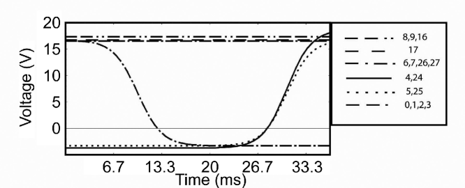
Figure 31: Control Electrode Voltage Profile to Separate Ions: Time dependant voltages applied on control electrodes in order to separate two ions initially held in a single harmonic trap at zone $b$ into two separate harmonic traps, one at $a$ and the other at $c$. Asymmetries in the voltage profile about $x=0$ are to compensate for misalignments in the electrode layers or stray fields. A time reversal of the above voltage profile allows us to combine two ions, one in trapping zone $a$ and the other at $c$, into a single harmonic trap at zone $b$.

The separation protocol implemented in the Michigan T-junction ion trap is illustrated in Fig. 31 [26]. The recombination protocol was a simple reversal of this voltage profile. Two ions were initially confined to a common trap at zone b. The trap is then weakened to extend over zones a, b, and c. Finally, the double-well (octupole) potential and separation of the ions is achieved by increasing the voltage on the electrodes that define the center of zone b (electrodes 4, 5, 24, and 25). Numerical simulations of this procedure indicate that the smallest trap frequency of the center of mass mode obtained is $\sim 27$ kHz. At this point, the distance between the two ions is found to be $\sim 64$ $\mu$m. Experimentally, the success rate of this separation protocol was $\sim 58$ % (64 attempts) for a total shuttling time of 10 ms.

Undoubtedly, the axial extent of the electrodes ($400$ $\mu$m) hindered the ability to efficiently separate ions given the 200 $\mu$m channel width. In general, the electrode widths should be of order the channel width. Others have reported near unit efficiency in ion separation in traps where the minimum axial extent of the electrodes was $400$ $\mu$m with a channel width of 400 $\mu$m [57]. The advent of micro-fabricated traps may allow for even finer control of the trapped ions [65, 59]. However, as indicated above, separation procedures appear to demand that the center of mass trap frequency be reduced for the creation of the octupole potential. Since motional heating has been shown to be inversely proportional to the trap frequency [52, 51] separation protocols may cause some additional heating as well.

5.5 Composite Protocols For Arbitrary Two Dimensional Control of Trapped Ions

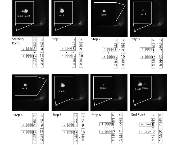
Figure 32: Images of two ions during the swapping protocol with schematics that indicate the ions’ positions in the trap. Two ions are initially trapped in zone d. They scatter a different number of photons because they are different isotopes and thus have two slightly different S_1/2 to P_3/2 transition frequencies due to the isotope shift. The ions make a three point turn by sending one ion around the corner one way and the other ion around the corner in the other direction after being separated inside the stem of the T. The two ions are brought back in the opposite order, effectively swapping the positions of the ions. This protocol makes use of linear shuttling, corner shuttling, separation, and recombination.

Linear shuttling, corner shuttling, separation, and recombination protocols may be combined to swap the positions of two ions that are initially trapped in the same trapping zone. The ability to perform all of these shuttling protocols in an ion trap array allows any two arbitrary ions to be brought together because a string of ions can be arbitrarily sorted. An application of this protocol would be the entanglement of two arbitrary ions inside a large ion string via two-ion quantum gates.

The step-wise process for the experimental implementation of a swapping protocol in the T-junction ion trap array is depicted in Fig. 32 [26]. Two ions are initially trapped in zone d. In order to distinguish the two ions, different isotopes are used. The two different isotopes have different S_1/2 to P_3/2 resonance frequencies, so the ions scatter a different number of photons when a detection laser is incident. The difference in photon scattering can be seen in the first panel of Fig. 32. The ions are shuttled to zone b where they are separated as described in the previous section. One ion (ion A) is shuttled to zone a while the other (ion B) is shuttled back to zone d where it is laser cooled. Ion B is then shuttled around the corner of the T-junction from zone d to zone i after which it is linearly shuttled to zone k (step 3 of Fig. 32) while ion A is shuttled from zone a to zone d where it is laser cooled. Ion A is then shuttled to zone i (where the ion is again laser cooled) after which it is shuttled through the junction to zone f. This three point turn is required since shuttling ions from zone d directly to zone f has not yet been accomplished (see Sec. 5.3.2). Ion A in zone f is then linearly shuttled to zone h. Ion B is shuttled back from zone k to zone i and then to zone d (step 5) where it can be laser cooled. Finally, ion A is shuttled to zone a. Ion A is then shuttled back from zone h to zone i where it can be laser cooled, and then ion A is shuttled to zone d. The two ions (in zones a and d) are then recombined in zone b and shuttled together to zone d where they are laser cooled and imaged. The net effect is that the ions have swapped places by executing a three point turn in the T-junction ion trap array.

This process is carried out in successive 10 ms steps and has an overall success rate of only 24% (51 attempts), but this low rate is mainly due to the the 58% success rate of the initial separation attempts and the final recombination attempts. Excluding the separation step at the beginning of the swapping protocol, the success rate of the remaining steps is 82% (34 attempts). Other than a failed separation, the main cause of a failed swapping protocol is that ions can swap places during the recombination step. Note that this protocol is carried out in successive 10 ms steps instead of as a continuous process. The reason that the swapping procedure was tested in a stepwise fashion was to ensure the success of each individual step of the protocol. The quoted 82% success rate may also be strongly dependent on laser cooling the ions whenever they are in zones d or i. Laser cooling serves to dissipate any additional energy and/or spread in the energy given to the ions during the shuttling procedures. Future work could characterize the success rate these protocols without implementing laser cooling during the swapping process.

6 Ion Transport in Three Dimensions

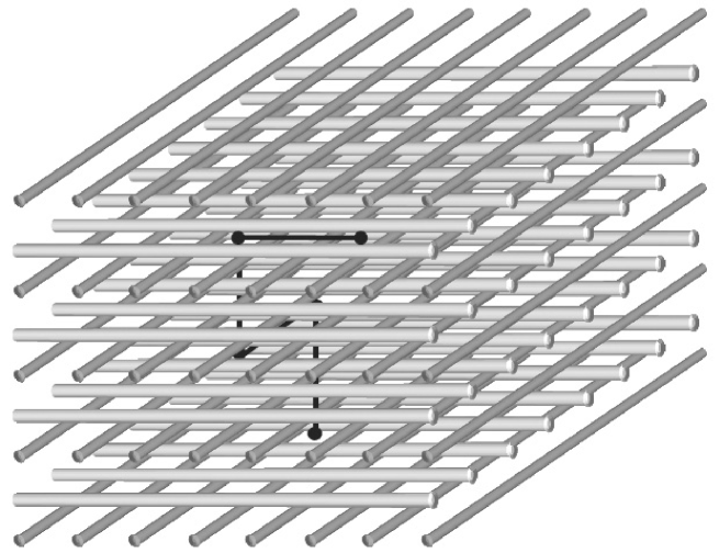
Figure 33: Schematic of a 3-dimensional ion trap array. Alternating layers of sets of parallel linear conductors run perpendicular to each other. One set of linear electrode layers (say, the lighter shaded electrodes running left-to-right) are meant to carry rf potentials, while the other (darker) electrode layers are meant to carry static potentials. Ions can be transported between any lattice point in between the grid of electrodes, in all three dimensions. Such a trap has been demonstrated with macroscopic charged dust particles, with 3-dimensional shuttling through a single layer and between layers.

In principle, trapped atomic ions can be transported in three dimensions, given a suitable trap geometry. The main advantage here is that space is used more efficiently, and for very large numbers of ions, using the third dimension would relax many constraints on the physical size of the collection of trapped ions. However, there are several practical issues concerning 3-dimensional trap channels. First, it may be difficult to gain optical access to submerged layers of trapping zones. Second, a 3-dimensional junction appears to have considerably more complexity than the 2-dimensional junctions considered earlier. Finally, the fabrication and electrical hookups in such a design may be particular challenging, especially if electrodes are completely submerged within the trap array. In this section, we nevertheless highlight a simple geometry amenable to 3-dimensional shuttling for completeness.

One example of a 3-dimensional array of ion trap zones is shown in Fig 33. Each layer is composed of a set of parallel line-conductors as electrodes, with alternating layers running in perpendicular directions. For the simplest case of three layers, the middle layer all carry equal rf potentials, and the outer layers carry static potentials. For more layers, this pattern is simply repeated. In this geometry, ions would be confined in the spaces between rf rails, as indicated in the figure. In addition to linear shuttling in a single layer, the ions can be transported through the gaps in between the static electrodes, and shuttled in 3-dimensions. Three-dimensional shuttling of macroscopic charged dust particles in such a trap was demonstrated at the University of Michigan [69].

7 Conclusion

We have discussed a wide range of issues that arise when considering the transport of atomic ions in linear and multi-dimensional ion trap arrays. We consider methods for calculating the dynamics of single atomic ions in the complex effective potentials arising from the shuttling process, and justify the use of classical trajectory treatments. We introduce the method of basis functions to efficiently account for the contribution from each of the trap electrodes to the electrostatic and ponderomotive potentials experienced by an ion being shuttled in such an array. We then show how these derived potentials can be used to obtain numerical simulations of the classical motion of a shuttled ion, using numerical methods such as the Bulirsch-Stoer method. Next, we provide a general theoretical framework for the shuttling process. This includes analytical expressions for the energy gain of the shuttled ions, accounting for both the inertial forcing of the ion due to changes in acceleration of the shuttling potential, and parametric forcing resulting from changes in the frequency of the shuttling potential. In order to minimize the added kinetic energy imparted to the shuttled ion, these considerations lead us to shuttling protocols that keep the shuttling potential at a fixed frequency and transport the ion following smooth trajectories such as a hyperbolic tangent path in time.

We pay particular attention to the implementation of junctions in both symmetric and asymmetric electrode geometries. When shuttling ions in two or more dimensions, an important issue we identified is the transport of ions through junction regions. The existence of rf holes, humps and energy barriers results in the need for sophisticated shuttling protocols. In order to reliably guide the ion through junctions, we find that the control electrodes near to the junction should be smaller than the characteristic channel width. This makes it possible to override the rf potential energy barriers in the junction region, allowing for the use of near-constant frequency shuttling potentials throughout the shuttling protocol.

We use experimental results on the Michigan T-junction trap [26] array and theoretical analysis of the process by which ions were shuttled through this T-junction in order to illustrate general principles in designing advanced shuttling protocols. All complicated shuttling processes are typically created from elementary sequences such as linear shuttling, corner turning, separation and recombination. We discuss the implementation of all of these processes in the particular case of this three-layer T-junction ion trap array and describe the implementation of a specific composite protocol, the three-point turn, along with a theoretical analysis.

The experiments in the T-junction trap array resulted in large amounts of kinetic energy following shuttling. Future work should allow shuttling in the strict adiabatic limit, where the quantum state of motion does not change appreciably after shuttling. This would involve either a more appropriate design of the ion trap electrodes to better control the ion through the junction, or the use of sympathetic cooling or phase sensitive switching of the trapping voltages. At the same time, we note that adiabaticity (or even confinement to the Lamb-Dicke limit) is not strictly necessary in certain quantum logic gate methods.

Shuttling ions in large scale arrays may form an important backbone for the implementation of an large-scale ion trap quantum processor. Progress in this field is lively, with several groups now working with various ion trap array geometries. In the future, the manipulation of hundreds or thousands of ions in large ion trap arrays will pose many more challenges such as appropriate device engineering, control electronics, motional control issues and ways to provide adiabatic but fast shuttling sequences. Mastering these challenges will require significant time and resources, but it is encouraging that none of the challenges seem to be of a fundamental nature.

8 Acknowledgments

We acknowledge useful discussions with M. Acton, J. Burress, M. Madsen, E.J. Otto, R. Slusher, D. Stick, J. Sterk, and D. Wineland. This work is supported by the National Security Agency and the Disruptive Technology Office under Army Research Office contract W911NF-04-1-0234, the National Science Foundation Information Technology Research (ITR) and Physics at the Information Frontier (PIF) Programs, and the UK Engineering and Physical Sciences Research Council (EP/E011136/1).

The purpose of this appendix is to illustrate the workings of numerical solver methods that may be useful in numerically solving Newton’s equations of motion in multizone ion trap arrays. Of particular importance is the Bulirsch-Stoer method which was used to develop the appropriate control electrode voltage profiles to guide ions around the corner of a T-junction ion trap [26].

Appendix A Explicit Runge-Kutta Methods

In general, numerical differential equation solvers try to solve first-order ordinary differential equations of the type

$$\frac{dx}{dt}=f(x,t),$$ (126)

There are many different classes of ODE solvers with their own merits. As a point of comparison, we introduce the familiar class of Explicit Runge-Kutta (ERK) methods. ERK methods are useful when only a low accuracy solution is required. In addition, if the potential gradient is rough or only roughly known so that the right hand side of Eq. 126 is not smooth, ERK Methods are usually more efficient [38]. In general, a Runge-Kutta method is of the form

$$x_{n+1}=x_{n}+h\Lambda(f,h,x_{n})$$ (127)

where $\Lambda$ is a function of $x_{n}$, the step size $h$ and the right hand side of equation 126.

The simplest version of an ERK method is Euler’s method. Euler’s method is given by

$$x_{n+1}=x_{n}+hf(t_{n},x_{n})$$ (128)

The interpretation of this method is simple; assuming the step size $h$ is small enough, the average rate of change of x over the time interval $(t_{n},t_{n+1}=t_{n}+h)$ is nearly equal to the rate of change at the start of the interval $\frac{dx(t_{n})}{dt}$. To characterize the local error of the Euler method, first consider the Taylor Expansion of $x$ about $t=t_{n}$ where $\alpha_{i}$ are the Taylor coefficients.

$$x(t_{n+1}=t_{n}+h)=x(t_{n})+\alpha_{1}h+\alpha_{2}h^{2}+...$$ (129)

If $x_{n}$ is the exact solution to the differential equation then the numerical estimation $x_{n+1}$, of $x(t_{n}+h)$ is given by

$$x_{n+1}=x_{n}+h\frac{dx}{dt}=x(t_{n})+\alpha_{1}h$$ (130)

The error that we get from a single step is

$$\epsilon=x(t_{n}+h)-x_{n+1}=\alpha_{2}h^{2}+\alpha_{3}h^{3}+...$$ (131)

This is the local error as defined in section 2.4. Euler’s method is accurate to first order because the lowest order contribution to the error is proportional to $h^{2}$.

A possible refinement to Euler’s method is to use the value of the derivative at the middle of the time interval at $t=\frac{t_{n}+t_{n+1}}{2}$. However, to calculate $f$ at $t=\frac{t_{n}+t_{n+1}}{2}$, it is necessary to calculate $x(\frac{t_{n}+t_{n+1}}{2})$, hence we use Equation 128 to take a trial step to estimate $x(t=\frac{t_{n}+t_{n+1}}{2})$.

$$x(\frac{t_{n}+t_{n+1}}{2})=x_{n}+\frac{h}{2}f(t_{n},x_{n})=z_{1}$$ (132)

We then use this intermediate point to calculate the rate of change and thus estimate the next node.

$$x_{n+1}=x_{n}+hf(t_{n}+h/2,z_{1})$$ (133)

Note that $z_{1}$ is the result of an intermediate calculation that can be discarded once $x_{n+1}$ is obtained. By using the Taylor expansion of $x$, the leading term of the local error is proportional to $h^{3}$ [38]. Therefore, this method is accurate to second order and is called the Second Order Runge-Kutta Method (RK2) or the Midpoint Method.

A general prescription to derive higher order Runge-Kutta methods is found in the literature [39]. One commonly used method is the Fourth Order Runge-Kutta Method (RK4). This method incorporates four intermediate steps in the process of obtaining the value of $x_{i+1}$:

$$x_{i+1} = x_{n}+\frac{h}{3}(\frac{g_{1}}{2}+g_{2}+g_{3}+\frac{g_{4}}{2})$$ (134)

$$g_{1} = f(t_{n},x_{n})$$ (135)

$$g_{2} = f(t_{n}+\frac{h}{2},x_{n}+\frac{g_{1}}{2})$$ (136)

$$g_{3} = f(t_{n}+\frac{h}{2},x_{n}+\frac{g_{2}}{2})$$ (137)

$$g_{4} = f(t_{n}+h,x_{n}+g_{3})$$ (138)

This method is 4th order accurate because the leading term in the error is proportional to $h^{5}$ [39]. In each step, RK4 does four evaluations of the function $f$ and is accurate to 4th order. By comparison, the Euler method does 1 evaluation of $f$ per step and is accurate to 1st order, and RK2 does 2 evaluations of $f$ and is accurate to 2nd order. ERK methods with order greater than 4 are therefore considered computationally inefficient because the number of evaluations of $f(x,t)$ is greater than the leading term in the error. RK4 has a good tradeoff in terms of accuracy and the computational efficiency since it is the highest order ERK method in which the accuracy order is the same as the number of evaluations of $f$ per step [39], and therefore has become the standard method for the numerical evaluation of ODEs.

Newton’s equations of motion for trapped ions are a set of second order ODEs, so in order for us to use the ERK method (or other ODE numerical solvers), the equations need to be reformulated into a system of 2k first order ODEs where k is the number of ions in the system.

$$\frac{d\mathbf{x_{j}}}{dt} = \mathbf{v_{j}}$$ (139)

$$\frac{d\mathbf{v_{j}}}{dt} = \mathbf{a}(\mathbf{x_{1}},...,\mathbf{x_{k}},t)$$ (140)

To simplify the notation, we define the following 3k-dimensional vectors where $\mathbf{X}$ denotes the positions of the k ions, $\mathbf{V}$ denotes the velocities of the k ions, and $\mathbf{A}$ denotes the accelerations of the k ions.

$$\mathbf{X}(t)=\left(\begin{array}[]{c}\mathbf{x}_{1}(t)\\ \vdots\\ \mathbf{x}_{k}(t)\end{array}\right);\hskip 7.22743pt\mathbf{V}(t)=\left(\begin{array}[]{c}\mathbf{v}_{1}(t)\\ \vdots\\ \mathbf{v}_{k}(t)\end{array}\right);\hskip 7.22743pt\mathbf{A}(\mathbf{x},t)=\left(\begin{array}[]{c}\mathbf{a}_{1}(\mathbf{x},t)\\ \vdots\\ \mathbf{a}_{k}(\mathbf{x},t)\end{array}\right).$$ (141)

The equations to calculate the next node are similar to Eq. 134 with the exception that the scalar quantities are replaced by vector quantities.

$$\left(\begin{array}[]{c}\mathbf{V_{n+1}}\\ \mathbf{X_{n+1}}\end{array}\right)\\ =\left(\begin{array}[]{c}\mathbf{V_{n}}\\ \mathbf{X_{n}}\end{array}\right)\\ +\frac{h}{3}\left[\frac{1}{2}\left(\begin{array}[]{c}\mathbf{g_{1}}\\ \mathbf{f_{1}}\end{array}\right)\\ +\left(\begin{array}[]{c}\mathbf{g_{2}}\\ \mathbf{f_{2}}\end{array}\right)\\ +\left(\begin{array}[]{c}\mathbf{g_{3}}\\ \mathbf{f_{3}}\end{array}\right)\\ +\frac{1}{2}\left(\begin{array}[]{c}\mathbf{g_{4}}\\ \mathbf{f_{4}}\end{array}\right)\right],$$ (142)

$$\mbox{where}\hskip 7.22743pt\left(\begin{array}[]{c}\mathbf{g_{1}}\\ \mathbf{f_{1}}\end{array}\right)\\ =\left(\begin{array}[]{c}\mathbf{A}(\mathbf{X_{n}},t_{n})\\ \mathbf{V_{n}}\end{array}\right),$$

$$\left(\begin{array}[]{c}\mathbf{g_{2}}\\ \mathbf{f_{2}}\end{array}\right)\\ =\left(\begin{array}[]{c}\mathbf{A}(\mathbf{X_{n}}+\frac{1}{2}h\mathbf{f_{1}},t_{n}+\frac{h}{2})\\ \mathbf{V_{n}}+\frac{h}{2}\mathbf{g_{1}}\end{array}\right),$$

$$\left(\begin{array}[]{c}\mathbf{g_{3}}\\ \mathbf{f_{3}}\end{array}\right)\\ =\left(\begin{array}[]{c}\mathbf{A}(\mathbf{X_{n}}+\frac{1}{2}h\mathbf{f_{2}},t_{n}+\frac{h}{2})\\ \mathbf{V_{n}}+\frac{h}{2}\mathbf{g_{2}}\end{array}\right),$$

$$\left(\begin{array}[]{c}\mathbf{g_{4}}\\ \mathbf{f_{4}}\end{array}\right)\\ =\left(\begin{array}[]{c}\mathbf{A}(\mathbf{X_{n}}+h\mathbf{f_{3}},t_{n}+h)\\ \mathbf{V_{n}}+h\mathbf{g_{3}}\end{array}\right).$$

An adaptive step size algorithm is almost always used in conjunction with the Runge-Kutta Method [39]. Therefore, it is necessary to estimate the local error in making each time-step. The error of the nodal value $\mathbf{V_{n+1}}$, $\mathbf{X_{n+1}}$ is estimated after each step $h$ via the method of RK pairs [39] which determines the difference between 4th and 5th order RK method results for $\mathbf{V_{n}}$ and $\mathbf{X_{n}}$. If the difference is within a pre-defined error goal, then the solver moves on to calculate the next node. Otherwise, the step size is reduced and the algorithm repeated until the error goal is met. In addition, more complicated versions of the Explicit Runge-Kutta solver also adaptively alter the order of the Runge-Kutta solver method. For example, one step may use the RK pair RK4 and RK5, while the next step may use RK2 and RK3.

Appendix B Bulirsch-Stoer Method

The Bulirsch-Stoer method is an ODE solver that yields high accuracy solutions efficiently [37]. However, if a low accuracy solution is desired or if the simulated forces on the particle are rough or discontinuous, this method is not as effective as the ERK [38]. The Bulirsch-Stoer method proved to be the most efficient and accurate ODE solver method for our purposes (see Section 2.4) and therefore, this method was our workhorse solver.

The Bulirsch-Stoer method seeks to obtain an accurate approximation of the nodal point $x_{i+1}$ from $x_{i}$ by first evaluating the derivatives of the solution at $n$ points evenly spaced throughout the time-step of size $H$, using the so-called Modified Midpoint method. The Bulirsch-Stoer method differs from the ERK class of methods in that this process is repeated for two or more different values of $n$, and therefore for several different sub-step sizes, $h=H/n$. As a result, several estimations $\chi_{i+1}(h=H/n)$ are made for the nodal point $(x_{i+1},t_{i}+H)$, each one characterized by the sub-step size, $H/n$. It is obvious that the smaller the sub-step size, the more accurate the approximation for the nodal point will be, with a limiting and presumably exact value, $\chi_{i+1}(0),$ obtained when the number of sub-steps goes to infinity. This limiting value would be prohibitively time-consuming and expensive to reach directly. However, by treating the various $\chi_{i+1}(h)$ as points on a polynomial function plotted versus $h^{2}=H^{2}/n^{2}$, it is possible to make a very accurate estimation of the value $\chi_{i+1}(0)$ by determining the y-intercept of this polynomial. This is done through the use of Richardson Extrapolation [37]. The Modified Midpoint method is well-suited for this approach because its local error is expressible as a power series in $h^{2}$ rather than $h$, meaning that $\chi_{i+1}(h)$ can be thought of as a function of $h^{2}$. Therefore, a reduction in sub-step size of 1/2 will result in obtaining a point in the polynomial four times closer to the y-intercept, making the estimate of $\chi_{i+1}(0)$ obtained by the Richardson Extrapolation far more accurate. Not only so, but the fact that $\chi_{i+1}(h)$ is an even function of the sub-step size $h$ means that this method is inherently time-reversible. This guarantees that the solutions obtained in this way satisfy an important constraint on solutions of Newton’s equations.

The Modified Midpoint method generates the initial crude estimates of the nodal point $\chi_{i+1}(h)$ that will be used for the Richardson extrapolation in order to calculate $x(t_{i}+H)$. The Modified Midpoint method advances across the time interval $(t_{i},t_{i+1})$ in a series of $n$ uniform sub-steps of size $h=H/n$. The equations for this method are

$$z_{0} = x_{i}$$

$$z_{1} = z_{0}+hf(t_{i},z_{0})$$

$$z_{m+1} = z_{m-1}+2hf(t_{i}+mh,z_{m})$$

$$\chi_{i+1}(h) = \frac{1}{2}[z_{n}+z_{n-1}+hf(t_{i}+H,z_{n})]$$ (143)

Every sub-step of the Modified Midpoint method calculates a value $z_{m}$. These values are intermediate calculations and will be discarded after finding the value of $x_{i+1}$. The Modified Midpoint method outlined above is similar to the Midpoint method given in Eq. 133, because in order to advance from the point $(t_{i}+mh,z_{m})$ to the point $(t_{i}+(m+2)h,z_{m+2})$, we use information from the derivative at the middle of the time interval, i.e. $f(t_{i}+(m+1)h,z_{m+1})$, to calculate the next point. However, the Modified Midpoint method is faster than the Midpoint method. If we had used the Midpoint method as our base ODE solver with the same sub-step size $h$, we would need to do $\frac{2H}{h}=2n$ evaluations of $f$. In contrast, the Modified Midpoint method only does $\frac{H}{h}+1=n+1$ such evaluations. As evaluations of $f$ are computationally expensive, the Modified Midpoint method is more efficient. The Modified Midpoint method has an additional advantage as the error contains only even powers of the step size $h$ [70], i.e.

$$\chi_{i+1}(h)-x(t_{i}+H)=\sum_{j=1}^{\infty}c_{j}\left(h\right)^{2j},$$ (144)

where the term $\sum_{j=1}^{\infty}c_{j}\left(\frac{H}{n}\right)^{2j}$ is the error, and $x(t_{i}+H)$ is the exact solution.

A significant improvement in accuracy can be obtained by employing the Modified Midpoint method several times over the Bulirsch-Stoer time step, $H$, each time with a different sub-step size, and then using each of those values to estimate the result were it to be run with an infinitesimally small sub-step size, $h\rightarrow 0$. For example, suppose that we have run the method $j$ times and as such have obtained $j$ points as follows

$$\{(h_{1}^{2},\chi(h_{1})),(h_{2}^{2},\chi(h_{2})),...,(h_{j}^{2},\chi(h_{j}))\}$$ (145)

There is a unique polynomial of order $j-1$ that passes through each of the $j$ points. For example, with two points, there is a unique linear polynomial, for three points, there is a unique quadratic, etc. This polynomial is given by Lagrange’s Formula

$$P(h^{2}) = \frac{(h^{2}-h_{2}^{2})(h^{2}-h_{3}^{2})...(h^{2}-h_{j}^{2})}{(h_{1}^{2}-h_{2}^{2})(h_{1}^{2}-h_{3}^{2})...(h_{1}^{2}-h_{j}^{2})}\chi(h_{1})+\frac{(h^{2}-h_{1}^{2})(h^{2}-h_{3}^{2})...(h^{2}-h_{j}^{2})}{(h_{2}^{2}-h_{1}^{2})(h_{2}^{2}-h_{3}^{2})...(h_{2}^{2}-h_{j}^{2})}\chi(h_{2})+...$$ (146)

$$+ \frac{(h^{2}-h_{1}^{2})(h^{2}-h_{2}^{2})...(h^{2}-h_{j-1}^{2})}{(h_{j}^{2}-h_{1}^{2})(h_{j}^{2}-h_{3}^{2})...(h_{j}^{2}-h_{j-1}^{2})}\chi(h_{j})$$

In order to complete the Richardson extrapolation, we need only read off the value $P(0)$ from this formula to obtain the next node. We note that equation 146 is a well-defined polynomial in $h^{2}$ due to equation 144. The advantage in doing so is that it gives more weight to the points with smaller $h$ in determining the value of $P(0)$ and greatly improves the accuracy of that calculation.

However, Eq. 146 has two disadvantages. First, it provides information about the entire polynomial whereas we are only interested in the value of the polynomial at $h^{2}=0$. Secondly, Eq. 146 provides no error estimate [71]. Therefore, Neville’s Algorithm [71] is used instead of Lagrange’s formula in the Bulirsch-Stoer algorithm to extrapolate the value of $\chi_{i+1}$ at $h^{2}=0$. Given our set of $j$ points, Neville’s Algorithm finds the value of $P(0)$ directly from the points obtained through the use of the Modified Midpoint Method, making Neville’s algorithm faster. In addition, Neville’s algorithm also provides a simple estimate of the error in the resulting value.

To illustrate Neville’s algorithm, we will fit the following three points to a second order polynomial and find the value of that polynomial at $h^{2}=0$. The three points are $(0.02250,1.34838),(5.625\times 10^{-3},1.34948),(2.500\times 10^{-3},1.34969)$. We begin by defining $P_{(1)}$ to be the value at $h^{2}=0$ of the unique zeroth-order polynomial (horizontal line) passing through the first point $P_{(1)}=1.34838$. $P_{(2)}$ and $P_{(3)}$ are defined similarly, so that $P_{(2)}=1.34948$ and $P_{(3)}=1.34969$. Next we define $P_{(1)(2)}$ to be the value at $h^{2}=0$ of the unique first-order polynomial that passes through the first two points. This value can be obtained from $P_{(1)}$ and $P_{(2)}$ using the following iterative equation:

$$P_{(i)(i+1)...(i+m)}=\frac{-h_{i+m}^{2}P_{i(i+1)...(i+m-1)}+h_{i}^{2}P_{(i+1)(i+2)...(i+m)}}{h_{i}^{2}-h_{i+m}^{2}}.$$ (147)

From Eq. 147 we can also derive the value of $P_{(2)(3)}$, the value at $h^{2}=0$ of the first order polynomial that passes through the second and third points. Our final value, $P_{(1)(2)(3)}$, is the value at $h^{2}=0$ of the unique second-order polynomial that passes through all three points. Again, $P_{(1)(2)(3)}$ can be derived from $P_{(1)(2)}$ and $P_{(2)(3)}$ via equation 147. An error estimate comes from the difference between the highest order estimate of $P(0)$ and the next highest order estimate of $P(0)$. For example, the error estimate of $P_{(1)(2)(3)}$ is given by

$$\epsilon=\frac{max\{|P_{(1)(2)(3)}-P_{(1)(2)}|,|P_{(1)(2)(3)}-P_{(2)(3)}|\}}{|P_{(1)(2)(3)}|}=6.4\times 10^{-6}.$$ (148)

Another advantage to Neville’s algorithm is that if we need to fit a new point into our polynomial, we need not recalculate all the values of $P$ from scratch. For example, if we add a fourth point to the above three points, we would only need to calculate $P_{(4)}$, $P_{(3)(4)}$, $P_{(2)(3)(4)}$ and $P_{(1)(2)(3)(4)}$. This improves the overall efficiency of the Bulirsch-Stoer Method.

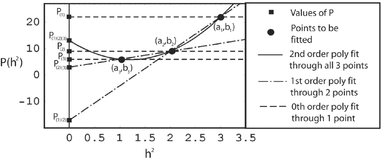
Figure 34: We demonstrate Neville’s algorithm for three random points $\{(a_{1},b_{1}),(a_{2},b_{2}),(a_{3},b_{3})\}$. The y intercept of the six polynomials give us the various $P$’s. Finally, Neville’s algorithm does not actually calculate the interpolating polynomials but only the y intercepts of the polynomials. The interpolating polynomials are added for illustrative purposes.

We are now ready to employ the Bulirsch-Stoer method to solve ordinary differential equations. We begin by finding rough estimates of $x(t_{i+1})$ with the Modified Midpoint Method using $n=2$ sub-steps and then $n=4$ sub-steps (Eq. 143). Next, we use Neville’s algorithm to calculate $\chi_{i+1}(0),$ and estimate the error (Eqs. 147 and 148). If we are within our error goals, we record the result and go on to calculate the next node. Otherwise, we obtain a third point, $(H^{2}/6^{2},\chi_{i+1}(H/6)$ using the Modified Midpoint method and repeat Neville’s algorithm using a second-order polynomial and check to see whether the error goal has been met. The sequence of numbers of sub-steps is $n=2,4,6,8,10,12,14,16,\ldots$. If the solution does not meet the error goals beyond a certain value of $n$, this would indicate that there is some unusual behavior within the time interval of the Bulirsch-Stoer step. Therefore, this sequence is usually terminated at the 8th iteration which corresponds to $n=16$ sub-steps. At that point, $H$ is reduced (usually halved) and the above procedure is repeated. A more detailed discussion of the adaptive step size algorithm is provided in the literature [38].

We now illustrate the Bulirsch-Stoer method by numerically solving a simple differential equation $\dot{x}(t)=x(t)$ with $x(0)=1$ so that $f(t,x)=x$. The exact solution to this differential equation is $x(t)=e^{t}$. For our example, we will take one large Bulirsch-Stoer step from $t=0$ to $t=0.3$, so that $H=0.3$. The result of this calculation will thus be a numerical estimate of the exact solution $x(t=0.3)$. We note that since the first node is given by initial conditions, $(t_{0}=0,x_{0}=1)$, we are trying to calculate the value $x_{1}\approx x(t=0.3)$.

Following the three-step algorithm that was outlined above, we first use the Modified Midpoint method to find $\chi_{1}(H/2)=1.34838$ and $\chi_{1}(H/4)=1.34948$, both evaluated to six significant figures. Note that the values used in our example of Neville’s algorithm are taken directly from this sample problem. Applying Richardson Extrapolation to these points, we obtain our first solution $x_{1}=P_{(1)(2)}=1.34985$ to six significant figures. We know that $e^{0.3}=1.34986$, to six significant figures, so the fractional difference of $\chi_{1}(H/2)$ from the exact solution is $1.1\times 10^{-3}$, while the fractional difference of $\chi_{1}(H/4)$ from the exact solution is $2.8\times 10^{-4}$. However, by applying Richardson Extrapolation to these two points to estimate $\chi_{1}(0)$, an extrapolated value is obtained which has a fractional difference from the exact result of $6.4\times 10^{-6}$. Thus, the extrapolation yields a result that is forty times more accurate than our raw estimates from the Modified Midpoint Method. Using the error estimation scheme given in Eq. 148, we estimate the fractional error to be $1.1\times 10^{-3}$. If this error is not acceptable, we then proceed to find the value of $\chi(H/6)=1.34969$ (six significant figures). The value $\chi_{1}(H/6)$ has a fractional difference of $1.2\times 10^{-4}$ from the exact answer. But when we apply Richardson Extrapolation to all three points, we obtain a value for $\chi_{1}(0)$ of $1.34986$, (six significant figures). This has a fractional difference from the exact value of $1.5\times 10^{-8}$. This result is roughly 10,000 times more accurate than our best $\chi_{1}$ value obtained directly from the Modified Midpoint Method, $\chi_{1}(H/6)$. The fractional local error estimate is given again by Eq. 148 and is $6.4\times 10^{-6}$. We note that in order to reach an accuracy of one part in $10^{8}$, the Bulirsch-Stoer algorithm only performs 12 evaluations of $f$. In order to reach the same accuracy using the Euler Method, we would need $3\times 10^{6}$ evaluations of $f$!

Substep size	Fract. diff.	Fract. diff after
	from Mod. Mid. Meth.	Richardson Extrapolation
$h=H/2$	$1.1\times 10^{-3}$	NA
$h=H/4$	$2.8\times 10^{-4}$	$6.4\times 10^{-6}$
$h=H/6$	$1.2\times 10^{-4}$	$1.5\times 10^{-8}$

Table 3: The first column refers to the fractional difference obtained in the numerical estimation of $x(t=0.3)$ and the exact solution. The second column shows the fractional difference after Richardson Extrapolation is applied. Notice that Richardson Extrapolation provides a huge increase in accuracy

To generalize the Bulirsch-Stoer method to solve Newton’s Equation for multiple ions (Eq. 18), we replace scalar quantities with vector quantities as was done for the ERK method. Given a node $(t_{i},\mathbf{V_{i}},\mathbf{X_{i}})$, we would like to calculate the next node $(t_{i+1}=t_{i}+H,\mathbf{V_{i+1}},\mathbf{X_{i+1}})$ with $\mathbf{V_{i+1}}$ approximating the exact velocities $\mathbf{V}(t_{i}+H)$ and $\mathbf{X_{i+1}}$ approximating the exact ion positions $\mathbf{X}(t_{i}+H)$.

$$\left(\begin{array}[]{c}\mathbf{\upsilon_{0}}\\ \mathbf{\Xi_{0}}\end{array}\right)\\ =\left(\begin{array}[]{c}\mathbf{V}(t_{i})\\ \mathbf{X}(t_{i})\end{array}\right)\\$$ (149)

$$\left(\begin{array}[]{c}\mathbf{\upsilon_{1}}\\ \mathbf{\Xi_{1}}\end{array}\right)\\ =\left(\begin{array}[]{c}\mathbf{\upsilon_{0}}\\ \mathbf{\Xi_{0}}\end{array}\right)\\ +h\left(\begin{array}[]{c}\mathbf{A}(\mathbf{\Xi_{0}},t_{i})\\ \mathbf{\upsilon_{0}}\end{array}\right)\\$$ (150)

$$\left(\begin{array}[]{c}\mathbf{\upsilon_{m+1}}\\ \mathbf{\Xi_{m+1}}\end{array}\right)\\ =\left(\begin{array}[]{c}\mathbf{\upsilon_{m-1}}\\ \mathbf{\Xi_{m-1}}\end{array}\right)\\ +2h\left(\begin{array}[]{c}\mathbf{A}(\mathbf{\Xi_{m}},t_{i}+mh)\\ \mathbf{\upsilon_{m}}\end{array}\right)$$ (151)

$$\\ \left(\begin{array}[]{c}\mathbf{\tilde{X}_{i+1}}(H^{2}/n^{2})\\ \mathbf{\tilde{V}_{i+1}}(H^{2}/n^{2})\end{array}\right)=\frac{1}{2}\left[\left(\begin{array}[]{c}\mathbf{\upsilon_{n}}\\ \mathbf{\Xi_{n}}\end{array}\right)\\ +\left(\begin{array}[]{c}\mathbf{\upsilon_{n-1}}\\ \mathbf{\Xi_{n-1}}\end{array}\right)\\ +h\left(\begin{array}[]{c}\mathbf{A}(\mathbf{\Xi_{n}},t_{i}+H)\\ \mathbf{\upsilon_{n}}\end{array}\right)\right]$$ (152)

$\mathbf{A}$ refers to the acceleration of the $k$ ions, and $\mathbf{\Xi_{i}}$, $\mathbf{\upsilon_{i}}$ are intermediate vectors that the modified midpoint method calculate at each sub-step. Once the calculation of each $\mathbf{X_{i+1}}$ and $\mathbf{V_{i+1}}$ is complete, the values $\mathbf{\Xi_{i}}$, $\mathbf{\upsilon_{i}}$ will be discarded.

$\mathbf{\tilde{X}_{i+1}}(H^{2}/n^{2})$ is the desired approximation to the exact solution $\mathbf{X}(t=t_{i}+H)$ and $\mathbf{\tilde{V}_{i+1}}(H^{2}/n^{2})$ is the desired approximation to the exact solution $\mathbf{V}(t=t_{i}+H)$. $\mathbf{\tilde{X}_{i+1}}$ and $\mathbf{\tilde{V}_{i+1}}$ are functions of $h^{2}$ where $h=H/n$ is the Modified Midpoint Method step size. Polynomial interpolation is carried out using Neville’s Algorithm (Eq. 147). However, each $P(h^{2})$ is now a $6k$-dimensional vector representing intermediate estimates of the position and velocity vectors. Finally, we need to generalize the error estimation scheme in order to implement our adaptive step size algorithm.

$$\mathbf{\epsilon}=\frac{max\{|\mathbf{P}_{(i)(i+1)\ldots(i+m)}-\mathbf{P}_{(i)(i+1)(i+m-1)}|,|\mathbf{P}_{(i)(i+1)\ldots(i+m)}-\mathbf{P}_{(i+1)(i+2)\ldots(i+m)}|\}}{|\mathbf{P}_{(i)(i+1)\ldots(i+m)}|}$$ (153)

Appendix C Stiff Systems and Backward Difference Formulas

The differential equation for a system of ions moving in an array of ion traps may be stiff as was discussed in Section 2.3. One way that stiffness can occur is if there are two very different time scales that govern the evolution of the solution to a differential equation. An example of a system of ODEs that is stiff is given by Press [38]:

$$u^{\prime}(t) = 998u+1998v$$

$$v^{\prime}(t) = -999u-1999v$$ (154)

The exact solutions to this system of ODEs with initial conditions $u(0)=1$ and $v(0)=0$ are

$$u(t) = 2e^{-t}-e^{-1000t}$$

$$v(t) = -e^{-t}+e^{-1000t}$$ (155)

The two terms in the solutions for $u(t)$ and $v(t)$ have vastly different timescales. Just after $t=0$, the $e^{-1000t}$ term dominates the evolution of the system, but near $t=1$, this term becomes negligible.

In order to illustrate the difficulties an explicit ODE solver has when handling a stiff system, we use the Euler Method, Eq. 128 to solve Eq. C. In matrix form, we may write this as

$$\left(\begin{array}[]{c}u_{n+1}\\ v_{n+1}\end{array}\right)\\ =\left(\begin{array}[]{c}u_{n}\\ v_{n}\end{array}\right)\\ -h\left(\begin{array}[]{cc}-998&-1998\\ 999&1999\end{array}\right)\\ \left(\begin{array}[]{c}u_{n}\\ v_{n}\end{array}\right)\\ \equiv(\mathbf{1}-h\mathbf{C})\left(\begin{array}[]{c}u_{n}\\ v_{n}\end{array}\right)\\$$ (156)

This simplifies to

$$\left(\begin{array}[]{c}u_{n}\\ v_{n}\end{array}\right)\\ =(\mathbf{1}-h\mathbf{C})^{n}\left(\begin{array}[]{c}u_{0}\\ v_{0}\end{array}\right)\\$$ (157)

Since the solutions for $u(t)$ and $v(t)$ both approach zero as a steady state solution, the numerical solution should also approach zero as a steady state solution. If the numerical solution exhibits any behavior that is qualitatively different, the numerical ODE solver is clearly be an unstable method. In order for the numerical solutions of Eq. C to approach 0, $(\mathbf{1}-h\mathbf{C})^{n}$ must converge to the zero matrix as $n\rightarrow\infty$ or equivalently [38]

$$h<\frac{2}{|\lambda_{max}|}=\frac{2}{1000}$$ (158)

where $|\lambda_{max}|$ is the largest absolute value of the eigenvalues of the matrix $\mathbf{C}$. The expression in Eq. 158 provides a strict upper-bound for the step size to be used when obtaining a numerical solution to the problem that is due entirely to stability concerns and not those of local error tolerances. For example, at $t=10$, we set our local error goal (the relative numerical error from one numerical step to the next, see equation 20) to be $\epsilon=10^{-6}$. To estimate the largest step size that we could take, we calculate a numerical estimate for $u$ and $v$ at $t=10+h$. This is derived from taking a single Euler step of size $h$ from the exact solution of Eq. C at $t=10$, i.e.

$$\left(\begin{array}[]{c}u(10+h)\\ v(10+h)\end{array}\right)\\ \approx\left(\begin{array}[]{c}u(10)\\ v(10)\end{array}\right)\\ -h\left(\begin{array}[]{cc}-998&-1998\\ 999&1999\end{array}\right)\\ \left(\begin{array}[]{c}u(10)\\ v(10)\end{array}\right)\\$$ (159)

The LHS of Equation 159 is the exact solution whilst the RHS is a numerical estimate of the exact solution at t=10+h. Therefore the difference between the LHS and RHS of Equation 159 is the local error. Using equation 159, we find that the largest step size allowable is $h=0.1$. However, equation 158 implies that we cannot take such a large step size as the qualitative behavior of the numerical solution (in our example, the long term behavior) will vastly differ from the exact solution and hence the Euler method will be unstable. Therefore, stiffness results in a loss of computational efficiency.

One way to to address this problem is to use implicit numerical methods   [40]. Although implicit numerical methods are generally more stable [38], it is more difficult to solve an implicit equation and this increases computational cost. For example, the Implicit Euler Method in one dimension is defined as follows

$$x_{n+1}=x_{n}+hf(t_{n+1},x_{n+1})$$ (160)

To illustrate how an implicit method is more robust than a typical explicit method, let us use the Implicit Euler Formula, 160, to solve the example given in C

$$\left(\begin{array}[]{c}u_{n+1}\\ v_{n+1}\end{array}\right)\\ =\left(\begin{array}[]{c}u_{n}\\ v_{n}\end{array}\right)\\ -h\left(\begin{array}[]{cc}-998&-1998\\ 999&1999\end{array}\right)\\ \left(\begin{array}[]{c}u_{n+1}\\ v_{n+1}\end{array}\right)\\$$ (161)

which simplifies to

$$\left(\begin{array}[]{c}u_{n}\\ v_{n}\end{array}\right)\\ =(\mathbf{1}+h\mathbf{C})^{-n}\left(\begin{array}[]{c}u_{0}\\ v_{0}\end{array}\right)\\$$ (162)

The eigenvalues of the matrix $(\mathbf{1}+h\mathbf{C})$ are $1/(1+h\lambda)$ which is always less than unity regardless of $h$, thus the matrix $(\mathbf{1}+h\mathbf{C})^{-n}$ will converge to the zero matrix as $n\rightarrow\infty$ regardless of $h$. Therefore, the Implicit Euler Method is more robust in this example. It also turns out that implicit methods give better stability for general ODEs [38]. However, the price to be paid for such stable behavior is that at every step, one needs to solve an implicit equation.

The Implicit Euler Method is the simplest member of the class of ODE solvers known as Backward Difference Formulae. The essential idea of the Backward Difference Formulae is to use polynomial extrapolation on previously calculated nodes to estimate the next node. For example, the second order Backward Difference Formula as used to solve equation 18 is

$$\left(\begin{array}[]{c}\mathbf{V_{n+1}}\\ \mathbf{X_{n+1}}\end{array}\right)\\ =\frac{4}{3}\left(\begin{array}[]{c}\mathbf{V_{n}}\\ \mathbf{X_{n}}\end{array}\right)\\ -\frac{1}{3}\left(\begin{array}[]{c}\mathbf{V_{n-1}}\\ \mathbf{X_{n-1}}\end{array}\right)\\ +\frac{2}{3}\left(\begin{array}[]{c}\mathbf{A}(\mathbf{X_{n+1}},t_{n}+h)\\ \mathbf{V}_{n+1}\end{array}\right)\\$$ (163)

Because it is implicit, each Backward Difference Formula step is usually more computationally expensive than a step in an explicit ODE solver like the Modified Midpoint Method. Nevertheless, when solving a stiff system it is usually better to use an implicit method rather than an explicit solver as the implicit method requires far fewer steps. The reduction in the number of steps has a stronger impact than the increased computational expense of an implicit method for each step. Therefore, when stiffness in an ODE is detected or suspected, the designer should switch to the Backward Difference Formulae. For example, Mathematica’s “NDSolve” uses the Adams Predictor Corrector Method by default and switches to a Backward Difference formula with an adaptive step-size and an adaptive order when stiffness is detected.

References

- [1] J.I. Cirac, and P. Zoller (1995), Quantum computation with cold, trapped ions, Phys. Rev. Lett., 74 (20), pp. 4091.
- [2] K. Mølmer and A. Sørensen (1999), Multiparticle entanglement of hot trapped ions, Phys. Rev. Lett., 82, pp. 1835.
- [3] D.J. Wineland, C. Monroe, W.M. Itano, D. Leibfried, B.E. King, and D.M. Meekhof (1998), Experimental issues in coherent quantum-state manipulation of trapped atomic ions, J. Res. NIST, 103, pp. 259-328.
- [4] Q. A. Turchette, C. S. Wood, B. E. King, C. J. Myatt, D. Leibfried, W. M. Itano, C. Monroe, and D. J. Wineland (1998), Deterministic Entanglement of Two Trapped Ions, Phys. Rev. Lett., 81, pp. 3631–34.
- [5] C. A. Sackett, D. Kielpinski, B. E. King, C. Langer, V. Meyer, C. J. Myatt, M. A. Rowe, Q. A. Turchette, W. M. Itano, D. J. Wineland and C. Monroe (2000), Experimental entanglement of four particles, Nature, 404, pp. 256.
- [6] C. F. Roos, M. Riebe, H. Häffner, W. Hänsel, J. Benhelm, G. P. T. Lancaster, C. Becher, F. Schmidt-Kaler, and R. Blatt (2004), Control and Measurment of Three-Qubit Entangled States, Science, 304, pp. 1478.
- [7] B. B. Blinov, D. L. Moehring, L.- M. Duan, and C. Monroe (2004), Observation of entanglement between a single trapped atom and a single photon, Nature, 428, pp. 153–157.
- [8] H. Häffner, F. Schmidt-Kaler, W. Hänsel, C.F. Roos, T. Körber, M. Chwalla, M. Riebe, J. Benhelm, U. D. Rapol, C. Becher, and R. Blatt (2005), Robust Entanglement, Appl. Phys. B, 81, pp. 151.
- [9] H. Häffner, W. Hänsel, C. F. Roos, J. Benhelm, D. Chek-al-kar, M. Chwalla, T. Körber, U. D. Rapol, M. Riebe, P. O. Schmidt, C. Becher, O. Gühne, W. Dür and R. Blatt (2005), Scalable multiparticle entanglement of trapped ions, Nature, 438, pp. 643.
- [10] D. Leibfried, E. Knill, S. Seidelin, J. Britton, R. B. Blakestad, J. Chiaverini, D. B. Hume, W. M. Itano, J. D. Jost, C. Langer, R. Ozeri, R. Reichle, and D. J. Wineland (2005), Creation of a six-atom ‘Schrodinger cat’ state, Nature, 438, pp. 639.
- [11] J. P. Home, M. J. McDonnell, D. M. Lucas, G. Imreh, B. C. Keitch, D. J. Szwer, N. R. Thomas, S. C. Webster, D. N. Stacey and A. M. Steane (2006), Deterministic entanglement and tomography of ion spin qubits, quant-ph/0603273.
- [12] C. Monroe, D. M. Meekhof, B. E. King, W. M. Itano, and D. J. Wineland (1995). Demonstration of a fundamental quantum logic gate, Phys. Rev. Lett., 75 (25), pp. 4714-17.
- [13] C. Monroe, D. Meekhof, B. E. King, and D. J. Wineland (1996), A Schrödinger Cat Superposition State of an Atom, Science 272, 1131.
- [14] B.L. DeMarco, A. Ben Kish, D. Leibfried, V. Meyer, M.A. Rowe, B.M. Jelenkovic, W.M. Itano, J. Britton, C. Langer, T. Rosenband, and D.J. Wineland (2002), Experimental Demonstration of a Controlled-NOT Wave-Packet Gate, Phys. Rev. Lett., 89, 267901.
- [15] D. Leibfried, B. DeMarco, V. Meyer, D. Lucas, M. Barrett, J. Britton, W. M. Itano, B. Jelenkovic, C. Langer, T. Rosenband, D. J. Wineland (2003), Experimental demonstration of a robust, high-fidelity geometric two ion-qubit phase gate, Nature, 422, pp. 412-415.
- [16] F. Schmidt-Kaler, H. Häffner, M. Riebe, S. Gulde, G.P.T. Lancaster, T. Deuschle, C. Becher, C. F. Roos, J. Eschner and R. Blatt (2003), Realization of the Cirac-Zoller controlled-NOT quantum gate, Nature, 422, pp. 408–411.
- [17] P.C. Haljan, P.J. Lee, K.-A. Brickman, M. Acton, L. Deslauriers, and C. Monroe (2005), Entanglement of Trapped-Ion Clock States, Phys. Rev. A, 72, 062316.
- [18] M.D. Barrett, J. Chiaverini, T. Schaetz, J. Britton, W. M. Itano, J. D. Jost, E. Knill, C. Langer, D. Leibfried, R. Ozeri, and D. J. Wineland (2004), Deterministic quantum teleportation of atomic qubits, Nature, 429, pp. 737–739.
- [19] M. Riebe, H. Häffner, C.F. Roos, W. Hänsel, J. Benhelm, G.P.T. Lancaster, T. W. Körber, C. Becher, F. Schmidt-Kaler, D. F. V. James and R. Blatt (2004), Deterministic quantum teleportation with atoms, Nature, 429, pp. 734–737.
- [20] S. Gulde, M. Riebe, G.P.T. Lancaster, C. Becher, J. Eschner, H. Häffner, F. Schmidt-Kaler, I.L. Chuang, and R. Blatt (2003), Implementing the Deutsch-Jozsa algorithm on an ion-trap quantum computer, Nature, 428, pp. 48–51.
- [21] J. Chiaverini, D. Leibfried, T. Schaetz, M. D. Barrett, R. B. Blakestad, J. Britton, W.M. Itano, J.D. Jost, E. Knill, C. Langer, R. Ozeri, and D.J. Wineland (2004), Realization of Quantum Error Correction, Nature, 432, pp. 602, 2004.
- [22] K.-A. Brickman, P. C. Haljan, P. J. Lee, M. Acton, L. Deslauriers and C. Monroe (2005), Implementation of Grover’s quantum search algorithm in a scalable system, Phys. Rev. A., 72, 050306.
- [23] J. Chiaverini, J. Britton, D. Leibfried, E. Krill, M. D. Barrett, R. B. Blakestad, W. M. Itano, J. D. Jost, C. Langer, R. Ozeri, T. Schaetz, and D. J. Wineland (2005), Implementation of the semiclassical quantum Fourier transform in a scalable system, Science, 308 (5724), pp. 997–1000.
- [24] R. Reichle, D. Leibfried, E. Knill, J. Britton, R.B. Blakestad, J. Jost, C. Langer, R. Ozeri, S. Seidelin, and D.J. Wineland (2006), Experimental purification of two-atom entanglement, Nature, 443, pp. 838–841.
- [25] D. Kielpinski, C. Monroe, and D. J. Wineland (2002), Architecture for a large-scale ion-trap quantum computer, Nature, 417, pp. 709.
- [26] W.K. Hensinger, S. Olmschenk, D. Stick, D. Hucul, M. Yeo, M. Acton, L. Deslauriers, J Rabchuk, and C. Monroe (2006), T-junction ion trap array for two-dimensional ion shuttling, storage, and manipulation, App. Phys. Lett., 88, 034101.
- [27] G.P. Berman and G.M. Zaslavsky (1978), Condition of stochasticity in quantum nonlinear systems, Physica (Amsterdam), 91A: pp. 450.
- [28] Z.P. Karkuszewski, J. Zakrzewski, and W.H. Zurek (2002), Breakdown of correspondence in chaotic systems: Ehrenfest versus localization times, Phys. Rev. A., 65, 042113.
- [29] D.J. Larson, J.C. Berquist, J.J. Bollinger, W.M. Itano, and D.J. Wineland (1986), Sympathetic cooling of trapped ions: A laser-cooled two species nonneutral ion plasma, Phys. Rev. Lett., 57, pp. 70–73.
- [30] H. Imajo, K. Hayasaka, R. Ohmukai, U. Tanaka, M. Watanabe, and S. Urabe (1996), High-resolution ultraviolet spectra of sympathetically-laser-cooled Cd+ ions, Phys. Rev. A., 53, pp. 122–125.
- [31] H. Rohde, S.T. Gulde, C.F. Roos, P.A. Barton, D. Leibfried, J. Eschner, F. Schmidt-Kaler, and R. Blatt (2001), Sympathetic ground-state cooling and coherent manipulation with two-ion crystals, J. Opt. B: Semiclassic. Opt., 3, pp. S34–S41.
- [32] B.B. Blinov, L. Deslauriers, P. Lee, M.J. Madsen, R. Miller, and C. Monroe (2002), Sympathetic cooling of trapped Cd+ isotopes, Phys. Rev. A, 65, 040304. M. Barrett,
- [33] B.L. DeMarco, T. Schaetz, V. Meyer, D. Leibfried, J. Britton, J. Chiaverini, W.M. Itano, B.M. Jelenkovic, J.D. Jost, C. Langer, T. Rosenband, and D.J. Wineland (20030, Sympathetic cooling of 9Be+ and 24Mg+ for quantum logic, Phys. Rev. A 68, 042302.
- [34] J.D. Jackson (1999), Classical Electrodynamics, 3rd ed., John Wiley & Sons (Hoboken, NJ), pp. 39.
- [35] H.H. Dehmelt (1967), Radio frequency spectroscopy of stored ion, Adv. At. Mol. Phys., 3, pp. 53.
- [36] G. Strang and G.J. Fix (1973), An Analysis of the Finite Element Method, Prentice-Hall, Inc. (Englewood Cliffs, N.J.), pp. 165–166.
- [37] R. Bulirsch, and J. Stoer (1966), Numerical treatment of ordinary differential equations by extrapolation methods, Numerische Mathematik, 8 (1), pp. 1–13.
- [38] W.H. Press, B. P. Flannery, S.A. Teukolsky and W. T. Vetterling (1992), Numerical Recipes in FORTRAN: The Art of Scientific Computing, 2nd ed., Cambridge University Press (Cambridge, England), ch. 16.
- [39] J. Leader (2004), Numerical Analysis and Scientific Computation. Addison Wesley (Boston, Massachussetts), ch. 6.
- [40] L.F. Shampine and C.W. Gear (1979), A Users view of Solving Stiff Ordinary Differential Equations, SIAM Review, 21, pp. 1–17.
- [41] S. Wolfram (1999), The Mathematica Book, 4th ed., Wolfram Media & Cambridge University Press (Champaign, Illinois; Cambridge, UK), pp. 1069, 1231.
- [42] R. Reichle, D. Leibfried, R.B. Blakestad, J. Britton, J. D. Jost, E. Knill, C. Langer, R. Ozeri, S. Sedelin, and D.J. Wineland (2006), Transport of single ions in segmented microstructured Paul trap arrays, Fortschritte der Physik, 54 (8–10), pp. 666.
- [43] S. Schulz, U. Poschinger, K. Singer, F. Schmidt-Kaler (2006), Optimzation of segmented linear Paul traps and transport of stored particles, Fortschritte der Physik, 54 (8-10), pp. 648–665.
- [44] K. Husimi (1953), Miscellanea in elementary quantum mechanics, II. Progr. Theor. Phys., 9, pp. 381–402.
- [45] E. H. Kerner (1958), Note on the forced and damped oscillator in quantum mechanics, Can. J. Phys., 36, pp. 371–377.
- [46] J.J. Sakurai (1994), Modern Quantum Mechanics, Rev. ed., Wiley (New York, New York), pp. 162–164.
- [47] M. Boas (2006), Mathematical Methods in the Physical Sciences, 3rd ed., Wiley (New York, New York), pp. 461–462.
- [48] A.M. Perelomov and V.S. Popov (1965), Method of generating functions for a quantum harmonic oscillator, Am. J. Phys., 33, pp. 537-544.
- [49] M. Abramowitz and I. Stegun (1964), Handbook of Mathematical Functions, Dover Publications (New York, NY), pp. 255, 559.
- [50] M. Abramowitz and I. Stegun (1964), Handbook of Mathematical Functions, Dover Publications (New York, NY), pp. 728–730.
- [51] Q.A. Turchette, D. Kielpinski, B.E. King, D. Leibfried, D.M. Meekhof, C.J. Myatt, M.A. Rowe, C.A. Sackett, C.S. Wood, W.M. Itano, C. Monroe, and D.J. Wineland (2000), Heating of trapped ions from the quantum ground state, Phys. Rev. A, 61, 063481.
- [52] L. Deslauriers, S. Olmschenk, W.K. Hensinger, J. Sterk, and C. Monroe (2006), Scaling and Suppression of Anamalous Heating in Ion Traps, Phys. Rev. Lett., 97, 103007.
- [53] D. L. Moehring, M. J. Madsen, K. C. Younge, R. N. Kohn, Jr., P. Maunz, L.-M. Duan, C. Monroe, and B. Blinov (2007), Quantum Networking with Photons and Trapped Atoms, J. Opt. Soc. Am. B 24, 300.
- [54] J. J. Garcia-Ripoll, P. Zoller, and J. I. Cirac (2003), Fast and robust two-qubit gates for scalable ion trap quantum computing, Phys. Rev. Lett. 91, 157901.
- [55] P. W. Shor (1995), Scheme for reducing decoherence in quantum computer memory, Phys. Rev. A, 52, R2493; A. M. Steane (1996), Error Correcting Codes in Quantum Theory, Phys. Rev. Lett., 77, pp. 793.
- [56] A. M. Steane (2003), Overhead and noise threshold of fault-tolerant quantum error correction, Phys. Rev. A, 68, 042322.
- [57] M. A. Rowe, A. Ben-Kish, B. DeMarco, D. Leibfried, V. Meyer, J. Beall, J. Britton, J. Hughes, W. M. Itano, B. Jelenkovic, C. Langer, T. Rosenband, and D. J. Wineland (2002), Transport of quantum states and separation of ions in a dual RF ion trap, Quantum Inf. and Comput., 2, pp. 257-271.
- [58] W. Hänsel, J. Reichel, P. Hommelhoff, and T.W. Hänsch (2001),Trapped-Atom Interferometer in a Magnetic Microtrap, Phys. Rev. A, 64, 063607(6).
- [59] D. Stick, W.K. Hensinger, S. Olmschenk, M.J. Madsen, K. Schwab, and C. Monroe (2006), Ion trap in a semiconductor chip, Nature Physics, 2, pp. 36.
- [60] M. Brownnutt, G. Wilpers, P. Gill, R.C. Thompson, and A.G. Sinclair (2006). Monolithic microfabricated ion trap chip design for scaleable quantum processors, New J. Phys, 8, 232.
- [61] M.J. Madsen, W.K. Hensinger, D. Stick, J.A. Rabchuk, and C. Monroe (2004), Planar ion trap geometry for microfabrication, Appl. Phys. B, 78, pp. 639.
- [62] L. Deslauriers, P. C. Haljan, P. J. Lee, K.-A. Brickman, B. B. Blinov, M. J. Madsen, and C. Monroe (2004), Zero-Point Cooling and Low Heating of Trapped Cd Ions, Phys. Rev. A, 70, 043408.
- [63] J. Chiaverini, R. B. Blakestad, J. Britton, J.D. Jost, C. Langer, D. Leibfried, R. Ozeri, and D. J. Wineland (2002), Surface-electrode architecture for ion-trap quantum information processing, Quantum Inf. and Comput., 2, pp. 257–271.
- [64] J. Kim, S. Pau, Z. Ma, H.R. McLellan, J.V. Gates, A. Kornblit, R.M. Jopson, I. Kang, M. Dinu, and R.E. Slusher (2005), System design for large-scale ion trap quantum information processor, Quantum Inf. and Comput., 5 (7), pp. 515–537.
- [65] J. Britton, D. Leibfried, J. Beall, R.B. Blakestad, J.J. Bollinger, J. Chiaverini, R.J. Epstein, J.D. Jost, D. Kielpinski, C. Langer, R. Ozeri, R. Reichle, S. Seidelin, N. Shiga, J.H. Wesenberg, and D.J. Wineland (2006), A microfabricated surface-electrode ion trap in silicon, quant-ph/0605170.
- [66] S. Seidelin, J. Chiaverini, R. Reichle, J.J. Bollinger, D. Leibfried, J. Britton, J. Wesenberg, R.B. Blakestad, R. J. Epstein, D. Hume, W. M. Itano, J. D. Jost, C. Langer, R. Ozeri, N. Shiga, and D.J. Wineland (2006), Microfabricated Surface-Electrode Ion Trap for Scalable Quantum Information Processing, Phys. Rev. Lett., 96, 253003.
-
[67]
R. E. Slusher (2006), 2006 TIQC Workshop, Boulder, CO
(http://tf.nist.gov/ion/workshop2006/slusher1.pdf) - [68] J.P. Home and A.M. Steane (2006), Electrode configurations for fast separation of trapped ions, Quantum Inf. and Comput., 6 (4 & 5), pp. 289–325.
- [69] E.J. Otto, University of Michigan, private communication.
- [70] W.B. Gragg (1965), On extrapolation algorithms for ordinary initial value problems, SIAM J. Numer. Anal., 2 (3), pp. 384–403.
- [71] W.H. Press, B. P. Flannery, S.A. Teukolsky and W. T. Vetterling (1992), Numerical Recipes in FORTRAN: The Art of Scientific Computing, 2nd ed., Cambridge University Press (Cambridge, England), pp. 108–109.