Non-monotonicity in the quantum-classical transition:
Chaos induced by quantum effects

Abstract

The transition from classical to quantum behavior for chaotic systems is understood to be accompanied by the suppression of chaotic effects as the relative size of $\hbar$ is increased. We show evidence to the contrary in the behavior of the quantum trajectory dynamics of a dissipative quantum chaotic system, the double-well Duffing oscillator. The classical limit in the case considered has regular behavior, but as the effective $\hbar$ is increased we see chaotic behavior. This chaos then disappears deeper into the quantum regime, which means that the quantum-classical transition in this case is non-monotonic in $\hbar$.

Open nonlinear quantum systems are critical in understanding the foundations of quantum behavior, particularly the transition from quantum to classical mechanics. For example, density matrix formulations have been used to argue that quantum systems decohere rapidly when the classical counterpart is chaotic, with the decoherence rate determined by the classical Lyapunov exponents of the systemzp . This applies to entanglement and fidelity issues as welljacquod ; jalabert ; arul , since decoherence amounts to entanglement with the environment.

A powerful alternative way of studying open quantum systems is the Quantum State Diffusion (QSD) approachpercival . This approach enabled the resolution of an important paradox, namely that in the absence of a QSD-like formulation, classical chaos cannot be recovered from quantum mechanics, indicating that the $\hbar\to 0$ limit is singular. Early QSD workbrun studied the convergence towards classical trajectories for a chaotic system, considering quantum Poincaré sections of the quantities $\langle\hat{x}\rangle$ and $\langle\hat{p}\rangle$. It showed that the classical chaotic attractor is recovered when the system parameters were such that $\hbar$ was small relative to the system’s characteristic action. As the relative $\hbar$ increased, the attractor disappeared gradually, suggesting a persistence of chaos into the quantum region, consistent with later, more quantitative analyses ota ; Adamyan . Related worksalman studied a quantum system that is being continuously weakly measured, which leads to similar equations as those for QSDSteck . This also showed that chaos is recovered in the classical limit, and that it persists, albeit reduced, substantially into the quantum regime. Another related study everitt of coupled Duffing oscillators, showed that quantum effects, specifically entanglement, persist in a quantum system even when the system is classical enough to be chaotic.

While the quantum persistence of chaos is interesting, it is still consistent with the understanding that chaos is a classical phenomenon that is suppressed quantum mechanically. Do quantum effects always decrease chaos, however? A closed Hamiltonian quantum system studied within a gaussian wavepacket approximation akp-schieve manifested chaos absent in its classical version. This has been understood to be an artifact of the approximation, since the full quantum system is not chaotic. Follow-up work with an open system liu-schieve also manifested quantum chaos, but it is not clear if this was not due to the approximations made.

In this paper we show the first (to the best of our knowledge) evidence of chaos being induced by quantum effects using QSD, whence there are no artifacts of approximations. Specifically, in a system with a non-chaotic classical limit, as we increase the relative $\hbar$, chaos emerges, due to explicitly quantum efffects (tunneling and zero-point energy) and as $\hbar$ is increased further, the chaos disappears. This intriguing result is arguably relatively common. More broadly, it shows that the quantum-classical transition for nonlinear systems is not a monotonic function of $\hbar$.

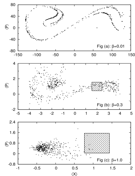
Figure 1: Poincaré sections for $\Gamma=0.125$, and $\beta=0.01,0.3,1.0$ reading from top to bottom. The monotonic transition from classical chaos to quantum regularity is to be contrasted with the non-monotonicity in Fig. (3). The shaded squares (area equal to $1$) in the center right of each graph indicate the Planck cell of size $\hbar$.

In QSD, the evolution equation for a realization $|\psi\rangle$ of the system interacting with a Markovian environment is

$$|d\psi\rangle = -\frac{i}{\hbar}\hat{H}|\psi\rangle dt$$ (1)

$$+ \sum_{j}\bigg{(}\langle\hat{L}_{j}^{\dagger}\rangle\hat{L}_{j}-\frac{1}{2}\hat{L}_{j}^{\dagger}\hat{L}_{j}-\frac{1}{2}\langle\hat{L}_{j}^{\dagger}\rangle\langle\hat{L}_{j}\rangle\bigg{)}|\psi\rangle dt$$

$$+ \sum_{j}(\hat{L}_{j}-\langle L_{j}\rangle)|\psi\rangle d\xi_{j}$$

where the Lindblad operators $\hat{L}_{j}$ model coupling to an external environment. The density matrix is recovered as the ensemble mean $M$ over different realizations as $\hat{\rho}=M|\psi\rangle\langle\psi|$percival . The $d\xi_{j}$ are independent normalized complex differential random variables satisfying $M(d\xi_{j})=0;M(d\xi_{j}d\xi_{j^{\prime}})=0;M(d\xi_{j}d\xi_{j^{\prime}})=\delta_{jj^{\prime}}dt$.

Now consider specifically the classical driven dissipative Duffing oscillator

$$\ddot{x}+2\Gamma\dot{x}+x^{3}-x=g\cos(\Omega t),$$ (2)

a particle of unit mass in a double-well potential, with dissipation $\Gamma$ dissipation, and a sinusoidal driving amplitude $g$. The dynamics depend on the parameters $\Gamma$, $g$ and $\Omega$, with chaotic behavior obtaining for certain parameter ranges. Chaos is found through Poincaré maps (obtained by recording $(x,\,p)$ at time intervals of $2\pi/\Omega$) showing a strange attractor, or the behavior of the time-series $x(t)$, or through a positive Lyapunov exponent. To quantize this problembrun ; ota , we choose the Hamiltonian $\hat{H}$ and the Lindblad operator $\hat{L}$ for Eq. (1) as $\hat{H}=\hat{H}_{D}+\hat{H}_{R}+\hat{H}_{ex}$,

$$\hat{H}_{D} = \frac{1}{2m}\hat{p}^{2}+\frac{m\omega^{2}_{0}}{4l^{2}}\hat{x}^{4}-\frac{m\omega^{2}_{0}}{2}\hat{x}^{2},$$ (3)

$$\hat{H}_{R} = \frac{\gamma}{2}(\hat{x}\hat{p}+\hat{p}\hat{x}),$$ (4)

$$\hat{H}_{ex} = -gml\omega_{0}^{2}\hat{x}\cos(\omega t),$$ (5)

$$\hat{L} = \sqrt{\frac{m\omega_{0}\gamma}{\hbar}}\;\hat{x}+\sqrt{\frac{\gamma}{m\omega_{0}\hbar}}\hat{p}$$ (6)

After some redefinitions this reduces to the dimensionless Hamltonian $\hat{H}_{\beta}$ and Lindblad operator $\hat{K}$ given by $\hat{H}_{\beta}=\hat{H}_{D}+\hat{H}_{R}+\hat{H}_{ex}$ where $\hat{H}_{D}=\frac{1}{2}\hat{P}^{2}+\frac{\beta^{2}}{4}\hat{Q}^{4}-\frac{1}{2}\hat{Q}^{2},\hat{H}_{R}=\frac{\Gamma}{2}\left(\hat{Q}\hat{P}+\hat{P}\hat{Q}\right),\hat{H}_{ex}=-\frac{g}{\beta}\hat{Q}\cos(\Omega t),\hat{K}=\sqrt{\Gamma}\left(\hat{Q}+i\hat{P}\right),$ and $\Omega\equiv\omega/\omega_{0}$, $\Gamma\equiv\gamma/\omega_{0}$. The quantity $\beta^{2}=\frac{\hbar}{ml^{2}\omega_{0}}$ determines the relative system size, and the degree to which quantum effects influence the motion. Specificallyota the limit $\beta\to 0$ yields the classical Eq (2) while increasing $\beta$ increases quantum corrections resulting in qualitatively different dynamics.

Figure 2: Low-frequency power spectra for the 3 $\beta$ values shown in Fig. (1), offset for visual clarity. We see the characteristic rise at low frequencieseveritt2 for the chaotic cases, as well as the monotonicity of the transition with $\beta$.

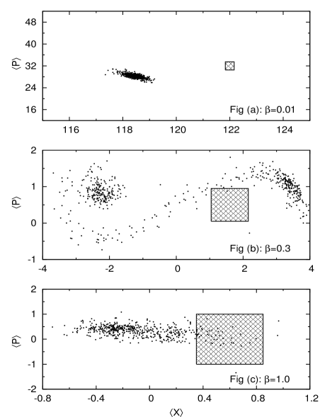
Figure 3: Poincaré sections for $\Gamma=0.3$, and $\beta=0.01,0.3,1.0$ reading from top to bottom. The non-monotonicity of {classical regularity $\to$ chaos $\to$ regularity} is to be contrasted with the monotonicity in Fig. (1).

Figure 4: Low-frequency power spectra for the 3 $\beta$ values shown in Fig. (3), offset for visual clarity. We see the characteristic rise at low frequencies for the chaotic case, as well as the non-monotonicity of the transition with $\beta$, to be contrasted with the monotonicity in Fig. (2).

Figure 5: Expectation values of energy and position for $\Gamma=0.125$, and $\beta=0.01,0.3,1.0$ reading from top to bottom, showing evidence for tunneling and the effect of zero-point energy as $\beta$ increases.

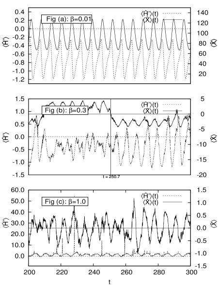
Figure 6: As in Fig.5 except that $\Gamma=0.3$, showing clearly that tunneling and the zero-point energy lead to bistability and chaos in this case.

We studied the quantum Duffing oscillator with simulations using the numerical QSD libraryQSD . Previous studiesbrun ; ota changed $\beta$, with the parameters $\Gamma=0.125$, $g=0.3$ and $\Omega=1.00$ held fixed. All these studies have the same classical limit, known to be chaoticGuckenheimer . We have studied $9$ different families of quantum systems, each with a different classical limit, and examined $13$ different values of $\beta$ from essentially classical ($\beta=0.01$) to the deep quantum regime ($\beta=1.0$). Of all these, we show six cases in the accompanying figures. Each simulation had the same initial state $|\psi(t=0)\rangle$ — the coherent state $|\sqrt{2}(\langle\hat{Q}\rangle+i\langle\hat{P}\rangle)=(1.4-0.4i)\rangle$ — and ran slightly over $500$ periods of the external driving, yielding $500$ post-transient points for the quantum Poincaré sections, shown for various $\beta$ in Fig. (1a,b,c) as inbrun ; ota . We next consider the low-frequency power spectra, shown in Fig. (2), from the Fourier transforms $\tilde{X}(\varpi)$ of the time-series $\langle\hat{Q}(t)\rangle$; we show plots smoothed via a cubic spline in Fourier space to focus attention on the overall trend.

We note both the broadband contributions of the noise in Eq. (1), and also an exponential increase in the power distribution in the low frequency ($\varpi\ll\Omega$) limit. This low frequency increase is characteristic of chaotic dynamics, and is absent in regular motion everitt2 . Now consider Figs. (3a,b,c), where we also show Poincaré sections, this time for $\Gamma=0.3$, $g=0.3$ and $\Omega=1.00$. In marked contrast to the $\Gamma=0.125$ situation, in this case we see the transition {regular $\to$ chaos $\to$ regular} as $\beta$ is increased. That is, the system becomes chaotic as quantal effects are increased, and then becomes regular again in the deep quantal region, as also evident in the power spectra in Fig. (4).

To understand these results, note that chaos occurs in this sort of system when trajectories sample the region near the unstable-fixed point, and particularly the separatrix region, leading to intra-well transitions. Classically, this means that a minimum amount of energy is needed for chaos to occur. The difference between (1a) and (3a) is due to the larger dissipation in (3a), confining the system to one well. The external driving force in the latter case is insufficient to overcome the potential barrier, and without this, chaos does not occur. Increasing $\beta$, however, increases the size of the wave-packet moving in the classical potential, adding extra degrees of freedom (along with the ‘classical’ centroid variables, there are now wave-packet variances) and changing how we understand the dynamics. It is in particular useful to build intuition by thinking of quantum mechanics as classical behavior in an effective potential. Increasing $\beta$ amounts to increasing quantum effects in the system effective potentialreale . These quantum corrections raise the effective bottom of the well through added zero-point energy and also modify the well-barrier, providing another route between the wells (tunneling).

These effects are apparent in time-slices of the expectation values of the energy operator, as well as position, in Figs. (5, 6). In Figs (5a,6a) we see classical behavior: transitions between wells only occur with positive energy. In Fig. (6a), the energy is always negative, confining the system in one well. In Figs. (5b,6b) quantum effects are significant and the barrier is softened as the zero-point energy becomes significant and the potential barrier at $x=0$ decreases. Now, transitions between wells occur even for negative energies, which we have indicated for (6b) with a line at $t=250.7$: this is quantum tunneling. Fig (6b) shows the core reason for the non-monotonic behaviour: classically forbidden inter-well transitions become possible due to quantum effects, allowing for chaos. Figs (5c,6c) show that in the deep quantum regime, the quantum effects are so large that the system effectively sees a single well potential leading to regular motion. Classically, changing $\beta$ is no more than changing the units of measurement for the system, or equivalently rescaling the system by a constant factor. Quantum dynamics however are sensitive to the absolute size of the system in units of $\hbar$. This scale dependence, rather than a variation of the dynamical parameters of the system as in classical chaos is what leads to the bifurcation signalling the onset of chaotic behaviour.

We have therefore seen that it is possible for the dynamics to be ‘quantum’ (as evidenced by tunneling effects) AND ’chaotic’ simultaneously, and specifically that the quantum effects in fact induce chaos. More broadly, quantum effects can be non-monotonic. It is likely that this is a generic property of nonlinear systems described by Hilbert space trajectories. Acknowledgements: AKP gratefully acknowledges the ‘SIT, Wallin, and Class of 1949’ sabbatical leave fellowships from Carleton.

References

- (1) W.H. Zurek and J.P. Paz, Phys. Rev. Lett. 72 2508 (1994).
- (2) R. Jalabert and H.M. Pastawski, Phys. Rev. Lett. 86 2490 (2001).
- (3) Ph. Jacquod, Phys. Rev. Lett. 92, 150403 (2004); C. Petijean and Jacquod, quant-ph/0510157.
- (4) P.A. Miller and S. Sarkar, Phys. Rev. E60, 1542 (1999); A. Lakshminarayan, Phys. Rev. E64, 036207 (2001).
- (5) I.C. Percival, Quantum State Diffusion (Cambridge University Press, Cambridge, England, 1998).
- (6) T.A. Brun, I.C. Percival, and R. Schack, J. Phys. A 29, 2077 (1996).
- (7) R. Schack, T. A. Brun and I. C. Percival, J. Phys. A 28, 5401 (1995); R. Schack and T. A. Brun Comput. Phys. Commun. 102, 210 (1997). This powerful software package integrates Eq.( 1), using a moving basis transformation, where advantage is taken of the solutions’ physical localization in Hilbert space, to achieve the algorithmic acceleration needed for complicated problems as consdered here.
- (8) Y. Ota and I. Ohba, Phys. Rev. E71, 015201(R) (2005); arxiv: quant-ph/0308154
- (9) H. H. Adamyan, S. B. Manvelyan, and G. Yu. Kryuchkyan, Phys. Rev. E64, 046219 (2001).
- (10) T. Bhattacharya, S. Habib, and K. Jacobs, Phys. Rev. Lett. 85, 4852 (2000); S. Habib, K. Jacobs and K. Shizume, Phys. Rev. Lett. 96, 010403 (2006).
- (11) See K. Jacobs and D. Steck, quant-ph/0611067.
- (12) M.J. Everitt et al New J. of Phys. 7, 64 (2005).
- (13) A.K. .Pattanayak and W.C. Schieve, Phys. Rev. Lett. 72, 2855 (1994)
- (14) W.V. Liu and W.C. Schieve, Phys. Rev. Lett. 78, 3278 (1997).
- (15) J. Guckenheiner and P. Holmes, Nonlinear Oscillators, Dynamical Systems and Bifurcations of Vector Fields (Springer, Berlin, 1983).
- (16) See similar power spectra for quantum chaos in M.J. Everitt et al Phys. Rev. E72, 066209 (2005).
- (17) D. O. Reale,A. K. Pattanayak, and W. C. Schieve, Phys. Rev. E51, 2925 (1995).