Global information balance in quantum measurements

Abstract

We perform an information-theoretical analysis of quantum measurement processes and obtain the global information balance in quantum measurements, in the form of a closed chain equation for quantum mutual entropies. Our balance provides a tight and general entropic information-disturbance trade-off, and explains the physical mechanism underlying it. Finally, the single-outcome case, that is, the case of measurements with post-selection, is briefly discussed.

It is now well-known that, even if Heisenberg uncertainty relations do not describe the disturbance caused on a quantum system by a quantum measurement ballentine ; ozawa11 ; dariano , Quantum Mechanics does indeed provide the existence of a monotonic information-disturbance relation: the more useful information is extracted from a quantum system, the more such a system is disturbed by the measurement. This fact is apparent from general arguments (if it were possible to gain information without causing disturbance, then it would be possible to determine the wave-function of an arbitrary system dariano-yuen ), as well as from some explicitly derived tradeoff relations obtained for some specific estimation tasks tradeoffs . On the other hand, proposals of reversible measurements have been reported invert , all of them implicitly based on the existence of a tradeoff between information extraction and probability of exact correction.

Despite the enormous relevance a universal relation between information extraction and disturbance due to a quantum measurement would have from both foundational and practical point of view, a general approach to the problem of quantifying such a relation, quite surprisingly, is still lacking. The main difficulty seems to be that explicitly known tradeoff relations involve quantities (like e. g. the average error probability or the average output fidelity) which strongly rely on the way the classical signals are encoded into quantum states, i.e. on the structure of the input ensemble. For this reason, the only known tradeoff curves cover some specific classes of ensembles enjoying symmetry properties, making the derivation possible tradeoffs .

The approach we propose in this Letter in order to overcome such a specificity, is to work with genuinely quantum entities. More explicitly, we will introduce a quantum information gain, which constitutes an upper bound to the information that the apparatus is able to extract, independently of how this information is encoded, and a quantum disturbance, which is related to the possibility of deterministically and coherently undoing the corresponding state change. Both quantum information gain and quantum disturbance are intimately related to previously known and independent notions: Groenewold’s information gain groene on one side, and channels coherent information schum-lloyd on the other, the latter applied by Maccone macca as a measure of disturbance, in the first attempt to “quantize” tradeoff relations. However, both of the quantities, as they were originally introduced, are not applicable to the most general situation. The definitions we introduce here, not only constitute a proper reformulation of these latter, but also allow us to elegantly link these (previously independent) quantities by using the chain rule for quantum mutual information only, thus establishing a closed information balance in quantum measurements. Such a balance provides, as a built-in feature, a tight and general entropic information-disturbance tradeoff relation. The same approach will be shown to be straightforwardly applicable also to the case of measurements with post-selection.

Quantum instruments.— A general measurement process $\mathscr{M}^{Q}$ on the input system $Q$, described by the input density matrix $\rho^{Q}$ on the (finite-dimensional) Hilbert space $\mathscr{H}^{Q}$, can be described as a collection of classical outcomes $\mathcal{X}:=\{m\}$, together with a set of completely positive (CP) maps $\{\mathcal{E}_{m}^{Q}\}_{m\in\mathcal{X}}$ kraus , such that, when the outcome $m$ is observed with probability $p(m):=\operatorname{Tr}[\mathcal{E}_{m}^{Q}(\rho^{Q})]$, $\sum_{m}p(m)=1$, the corresponding a posteriori state $\rho^{Q^{\prime}}_{m}:=\mathcal{E}_{m}^{Q}(\rho^{Q})/p(m)$ is output by the apparatus. This is the CP quantum instruments formalism introduced by Ozawa ozawa-instr (). With a little abuse of notation, we can think that the action of the measurement $\mathscr{M}^{Q}$ on $\rho^{Q}$ is given in average by the mapping

$$\begin{split}\mathscr{M}^{Q}(\rho^{Q})&:=\sum_{m}p(m)\rho^{Q^{\prime}}_{m}\otimes m^{\mathcal{X}}\\ &:=\Theta^{Q^{\prime}\mathcal{X}},\end{split}$$ (1)

where $\{|m^{\mathcal{X}}\rangle\}_{m}$ is a set of orthonormal (hence perfectly distinguishable) vectors on the classical register space $\mathcal{X}$ of outcomes. If the outcomes are discarded before being read out, that is, if $\Theta^{Q^{\prime}\mathcal{X}}$ in Eq. (1) is traced over $\mathcal{X}$, then the resulting average map $\mathcal{E}^{Q}:=\sum_{m}\mathcal{E}^{Q}_{m}$ is a channel, i. e. a CP trace-preserving (TP) map: quantum instruments contain quantum channels as a special case. If, on the other hand, we are not interested in the a posteriori states but only in the outcomes probability distribution $\vec{p}(m)$ (that is equivalent to tracing $\Theta^{Q^{\prime}\mathcal{X}}$ over $Q^{\prime}$), then the resulting average map $\rho^{Q}\mapsto\vec{p}(m)$ is described by a Positive Operator Valued Measure (POVM), namely, a set of positive operators $\{P^{Q}_{m}\}_{m\in\mathcal{X}}$, $\sum_{m}P^{Q}_{m}=\openone^{Q}$, such that $p(m)=\operatorname{Tr}[\rho^{Q}P^{Q}_{m}]$: quantum instruments contain POVMs as a special case.

We now exploit a very useful representation theorem for CP quantum instruments ozawa-instr : it states that whatever quantum measurement can be modeled as an indirect measurement, in which the input system first interacts with an apparatus (or probe) $A$, initialized in a fixed pure state $\phi^{A}$, through a suitable unitary interaction $U^{QA}:QA\to Q^{\prime}A^{\prime}\simeq QA$; subsequently, a particular measurement $\mathscr{M}^{A^{\prime}}$, depending also on $U^{QA}$, is performed on the apparatus. In addition, by introducing a third reference system $R$ purifying the input state as $\Psi^{RQ}$, $\operatorname{Tr}_{R}[\Psi^{RQ}]=\rho^{Q}$, we are in the situation schematically represented as in FIG. 1: right after the unitary interaction $U^{QA}$, the global tripartite state is $|\Upsilon^{RQ^{\prime}A^{\prime}}\rangle:=(\openone^{R}\otimes U^{QA})(|\Psi^{RQ}\rangle\otimes|\phi^{A}\rangle)$, and the measurement on the apparatus can be chosen such that 

$$\begin{split}(\operatorname{id}^{RQ^{\prime}}\otimes\mathscr{M}^{A^{\prime}})(\Upsilon^{RQ^{\prime}A^{\prime}})&:=\sum_{m}p(m)\Upsilon^{RQ^{\prime}A^{\prime\prime}}_{m}\otimes m^{\mathcal{X}}\\ &:=\Theta^{RQ^{\prime}A^{\prime\prime}\mathcal{X}},\end{split}$$ (2)

where $\Upsilon^{RQ^{\prime}A^{\prime\prime}}_{m}$ are pure states such that $\operatorname{Tr}_{A^{\prime\prime}}[\Upsilon^{RQ^{\prime}A^{\prime\prime}}_{m}]=(\operatorname{id}^{R}\otimes\mathcal{E}^{Q}_{m})(\Psi^{RQ})/p(m)=:\rho^{RQ^{\prime}}_{m}$ and $\operatorname{Tr}_{R}[\rho^{RQ^{\prime}}_{m}]=\rho^{Q^{\prime}}_{m}$, and $m^{\mathcal{X}}$ are the classical register states, as before. The above equation is nothing but a particular extension of Eq. (1): in fact, by tracing $\Theta^{RQ^{\prime}A^{\prime\prime}\mathcal{X}}$ over $R$ and $A^{\prime\prime}$, one obtains the state $\Theta^{Q^{\prime}\mathcal{X}}$ in Eq. (1). (For this reason, in the following, where no confusion arises, we will adopt the convention that to omit indices in the exponent of a multipartite state means to trace over the omitted indices.) Even though it is a simple rewriting, Eq. (2) will turn out to be very useful for our analysis, in that it gives a deeper insight in understanding the overall information balance.

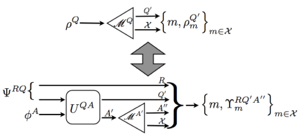
Figure 1: The action of a quantum measurement $\mathscr{M}^{Q}$ on the input state $\rho^{Q}$ (top), can always be extended as a tripartite indirect measurement (bottom), where the apparatus $A$, after having properly interacted with the input system through $U^{QA}$, undergoes the measurement $\mathscr{M}^{A^{\prime}}$. The conditional output pure states $\{\Upsilon^{RQ^{\prime}A^{\prime\prime}}_{m}\}_{m}$ are such that $\operatorname{Tr}_{RA^{\prime\prime}}[\Upsilon^{RQ^{\prime}A^{\prime\prime}}_{m}]=\rho^{Q^{\prime}}_{m}$, $\forall m$. See Eqs. (1) and (2) in the text.

Quantum information gain.— Having in mind Eq. (2), we define the (quantum) information gain $\iota(\rho^{Q},\mathscr{M}^{Q})$ of the measurement $\mathscr{M}^{Q}$ on the input state $\rho^{Q}$ as

$$\iota(\rho^{Q},\mathscr{M}^{Q}):=I^{R:\mathcal{X}}(\Theta^{R\mathcal{X}}),$$ (3)

where $I^{A:B}(\sigma^{AB}):=S(\sigma^{A})+S(\sigma^{B})-S(\sigma^{AB})$ is the usual quantum mutual information mutual_info . Due to the particular form of $\Theta^{RQ^{\prime}A^{\prime\prime}\mathcal{X}}$, it is possible to rewrite such a quantity as $\iota(\rho^{Q},\mathscr{M}^{Q})=S(\rho^{R})-\sum_{m}p(m)S(\rho^{R}_{m})$, for $\rho^{R}_{m}:=\operatorname{Tr}_{Q^{\prime}}[\rho^{RQ^{\prime}}_{m}]$. In other words, $\iota(\rho^{Q},\mathscr{M}^{Q})$ is the $\chi$-quantity chi of the ensemble induced on the system $R$ by the measurement $\mathscr{M}^{Q}$. In communication theory in fact, the information gain is usually better understood as being about the remote system $R$, while $Q$, correlated with $R$, represents just the carrier that is measured. Nonetheless, it is a crucial point, for what follows, that the information gain (3) only depends on the input state $\rho^{Q}$ and on the measurement $\mathscr{M}^{Q}$ performed onto it, regardless of the particular extension constructed in Eq. (2), . Indeed $\iota(\rho^{Q},\mathscr{M}^{Q})$ depends only on the input state $\rho^{Q}$ and on the POVM $\{P^{Q}_{m}\}_{m\in\mathcal{X}}$ induced by $\mathscr{M}^{Q}$, regardless of the particular state reduction maps $\{\mathcal{E}^{Q}_{m}\}_{m\in\mathcal{X}}$ and of the explicit form of the a posteriori states $\{\rho^{Q^{\prime}}_{m}\}_{m\in\mathcal{X}}$.

Holevo’s upper bound holevo on the accessible information provides a clear interpretation of our definition of information gain: $\iota(\rho^{Q},\mathscr{M}^{Q})$ is the Holevo bound to the amount of classical information which can be reliably extracted by the measurement $\mathscr{M}^{Q}$ from the input state $\rho^{Q}$. In fact, consider whatever classical alphabet $X:=\{x\}$, however encoded on the input state as $\rho^{Q}=\sum_{x}\rho^{Q}_{x}$: in this case, the joint input-output probability distribution is given by $p(x,m)=\operatorname{Tr}[\mathcal{E}_{m}^{Q}(\rho^{Q}_{x})]$. On the other hand, every such an encoding can be (formally) seen as induced by the measurement of a suitable POVM over the reference system $R$, in formula, $\rho^{Q}_{x}=\operatorname{Tr}_{R}[(P^{R}_{x}\otimes\openone^{Q})\Psi^{RQ}]$, for some POVM $\{P^{R}_{x}\}_{x\in X}$. This means that we can also write $p(x,m)=\operatorname{Tr}[\rho^{R}_{m}P^{R}_{x}]$, implicitly considering a “dual” situation, in which the encoded input is $m$ and the decoded letter is $x$. It is clear then, that the classical mutual information $I(X:\mathcal{X})$—which is a symmetric function of its arguments—between the alphabet $X$ and the indices in $\mathcal{X}$ is upper bounded by the $\chi$-quantity of the ensemble $\{p(m),\rho^{R}_{m}\}_{m\in\mathcal{X}}$ which exactly corresponds to $\iota(\rho^{Q},\mathscr{M}^{Q})$. In formula: $I(X:\mathcal{X})\leq\iota(\rho^{Q},\mathscr{M}^{Q})$.

It is interesting here to compare our definition of information gain to the one dating back to Groenewold groene (and which, by the way, was never put in relation with whatsoever notion of disturbance). He defined the information gain for von Neumann-Lüders measurements to be equal to $\iota_{G}(\rho^{Q},\mathscr{M}^{Q}):=S(\rho^{Q})-\sum_{m}p(m)S(\rho^{Q^{\prime}}_{m})$, conjecturing its positivity. Later Ozawa ozawa generalized Groenewold’s definition to take into account all possible measurements and characterized those with $\iota_{G}\geq 0$, explicitly pointing out that the general quantum instruments formalism commonly allows situations where $\iota_{G}<0$. This feature, making the interpretation of $\iota_{G}$ as an information gain problematic, comes from the fact that Groenewold-Ozawa definition, contrarily to ours, explicitly depends on the particular a posteriori states $\{\rho^{Q^{\prime}}_{m}\}_{m\in\mathcal{X}}$. Nonetheless, there are situations (to be shown in the following) where $\iota_{G}(\rho^{Q},\mathscr{M}^{Q})=\iota(\rho^{Q},\mathscr{M}^{Q})$. Incidentally, our definition of information gain (3) always returns the same numerical value of Winter’s “intrinsic information” of a POVM Winter , thus gaining an operational interpretation, and of Hall’s “dual upper bound” on accessible information Hall , even if their definitions slightly differ from ours.

Quantum disturbance.— As we anticipated in the introduction, our notion of disturbance is closely related to that of coherent information. A first step in this direction is due to Maccone macca , who however used a different definition, not suitable for the case of general quantum measurements. We define the (quantum) disturbance $\delta(\rho^{Q},\mathscr{M}^{Q})$ caused by the measurement $\mathscr{M}^{Q}$ on the input state $\rho^{Q}$ as

$$\delta(\rho^{Q},\mathscr{M}^{Q}):=S(\rho^{Q})-I_{c}^{R\to Q^{\prime}\mathcal{X}}(\Theta^{RQ^{\prime}\mathcal{X}}),$$ (4)

where $I_{c}^{A\to B}(\sigma^{AB}):=S(\sigma^{B})-S(\sigma^{AB})$ is the so-called coherent information schum-lloyd . In the following we will show the reason why the quantity $\delta(\rho^{Q},\mathscr{M}^{Q})$ can be understood as the disturbance.

Given a quantum channel $\mathcal{E}^{Q}$, from $Q$ to $Q^{\prime}$, acting on the input state $\rho^{Q}$, it is known that the coherent information $I_{c}^{R\to Q^{\prime}}((\operatorname{id}^{R}\otimes\mathcal{E}^{Q})(\Psi^{RQ}))$ plays a central role in quantifying how well the channel preserves quantum coherence. In fact, coherent information turns out to be intimately related to the possibility of constructing a recovering operation $\mathcal{R}^{Q^{\prime}}$, from $Q^{\prime}$ to $Q$, correcting the action of $\mathcal{E}^{Q}$: the closer the coherent information is to its maximum value $S(\rho^{Q})$, the closer (on the support of $\rho^{Q}$) the corrected channel $\mathcal{R}^{Q^{\prime}}\circ\mathcal{E}^{Q}$ is to the ideal channel $\operatorname{id}^{Q}$. In particular, in Ref. schumacher-westmoreland it is proved that whenever $S(\rho^{Q})-I_{c}^{R\to Q^{\prime}}((\operatorname{id}^{R}\otimes\mathcal{E}^{Q})(\Psi^{RQ}))\leq\epsilon$, then it is possible to explicitly construct a correcting channel (generally depending also on $\rho^{Q}$, but for sake of clarity of notation, we will drop such dependence, leaving it understood) $\mathcal{R}^{Q^{\prime}}$ such that $F_{e}(\rho^{Q},\mathcal{R}^{Q^{\prime}}\circ\mathcal{E}^{Q})\geq 1-2\sqrt{\epsilon}$, where $F_{e}(\rho^{Q},\mathcal{R}^{Q^{\prime}}\circ\mathcal{E}^{Q}):=\langle\Psi^{RQ}|(\operatorname{id}^{R}\otimes\mathcal{R}^{Q^{\prime}}\circ\mathcal{E}^{Q})(\Psi^{RQ})|\Psi^{RQ}\rangle$ is the entanglement fidelity schum of the corrected channel $\mathcal{R}^{Q^{\prime}}\circ\mathcal{E}^{Q}$ with respect to the input state $\rho^{Q}$. The value of $F_{e}(\rho^{Q},\mathcal{R}^{Q^{\prime}}\circ\mathcal{E}^{Q})$ says how close is the corrected channel $\mathcal{R}^{Q^{\prime}}\circ\mathcal{E}^{Q}$ to the identity channel $\operatorname{id}^{Q}$ on the support of $\rho^{Q}$. If such value is close to one, it means not only that $\mathcal{R}^{Q^{\prime}}(\mathcal{E}^{Q}(\rho^{Q}))$ is close to $\rho^{Q}$, but also that quantum correlations between $Q$ and $R$ are almost preserved.

The correction exploited in Ref. schumacher-westmoreland is blind, in the sense that the channel $\mathcal{R}^{Q^{\prime}}$ is a fixed one and works well on the average channel $\mathcal{E}^{Q}$. In our setting, on the contrary, the indices $m$ are by definition visible, in that they are the outcomes of the measurement: this fact reflects the form of Eq. (4), where the output $Q^{\prime}$ is considered jointly with the outcomes space $\mathcal{X}$. Then, following schumacher-westmoreland , a fixed correcting channel $Q^{\prime}\mathcal{X}\to Q$ results in a family of correcting channels $\mathcal{R}_{m}^{Q^{\prime}}:Q^{\prime}\to Q$, depending on the measurement readout $m$. We thus obtained the following

Theorem 1 (Approx. measurement correction)

If $\delta(\rho^{Q},\mathscr{M}^{Q})\leq\epsilon$, then there exists a family of recovering operations $\{\mathcal{R}_{m}^{Q^{\prime}}\}_{m\in\mathcal{X}}$ such that

$$F_{e}(\rho^{Q},\sum_{m}\mathcal{R}_{m}^{Q^{\prime}}\circ\mathcal{E}^{Q}_{m})\geq 1-2\sqrt{\epsilon}.\qquad\square$$

It is worth stressing that also the converse statement is true, namely, an approximately reversible instrument is almost undisturbing. In fact, as proved in Ref. barnischu , a sort of quantum Fano inequality holds for every set of channels $\{\mathcal{R}_{m}^{Q^{\prime}}\}_{m\in\mathcal{X}}$, in that $\delta(\rho^{Q},\mathscr{M}^{Q})\leq\operatorname{f}[1-F_{e}(\rho^{Q},\sum_{m}\mathcal{R}_{m}^{Q^{\prime}}\circ\mathcal{E}^{Q}_{m})]$, where $\operatorname{f}(x)$ is an appropriate positive, continuous, monotonic increasing function such that $\operatorname{f}(0)=0$.

As we said, our definition of disturbance (4) generalizes the usual notion of coherent information loss for quantum channels, which can be recovered from our formula (4) by simply tracing over the outcomes space $\mathcal{X}$, thus obtaining the quantity $S(\rho^{Q})-I_{c}^{R\to Q^{\prime}}(\Theta^{RQ^{\prime}})$, which, thanks to the data-processing inequality, is always greater than or equal to $S(\rho^{Q})-I_{c}^{R\to Q^{\prime}\mathcal{X}}(\Theta^{RQ^{\prime}\mathcal{X}})$. In other words, when discarding the outcomes (as done in Ref. macca ), the disturbance is higher, thus providing a too much loose tradeoff. The importance of taking into account the measurement outcomes during the correction is then clear bus .

Global information balance.— Before proceeding, let us explicitly calculate the disturbance (4) for the state $\Theta^{RQ^{\prime}A^{\prime\prime}\mathcal{X}}$: because of the classical feature of $\mathcal{X}$, we find

$$\delta(\rho^{Q},\mathscr{M}^{Q})=I^{R:A^{\prime\prime}\mathcal{X}}(\Theta^{RA^{\prime\prime}\mathcal{X}}).$$ (5)

Then, by using the chain rule for quantum mutual information hayashi , valid for all tripartite states $\sigma^{ABC}$, that is $I^{A:C}(\sigma^{AC})+I^{A:B|C}(\sigma^{ABC})=I^{A:BC}(\sigma^{ABC})$, where $I^{A:B|C}(\sigma^{ABC}):=S(\sigma^{AC})+S(\sigma^{BC})-S(\sigma^{ABC})-S(\sigma^{C})$ is the quantum conditional mutual information, we can put together Eqs. (3) and (5), thus obtaining the global balance of information in a quantum measurement as

$$\iota(\rho^{Q},\mathscr{M}^{Q})+\Delta(\rho^{Q},\mathscr{M}^{Q})=\delta(\rho^{Q},\mathscr{M}^{Q}).$$ (6)

The positive quantity

$$\begin{split}\Delta(\rho^{Q},\mathscr{M}^{Q})&:=I^{R:A^{\prime\prime}|\mathcal{X}}(\Theta^{RA^{\prime\prime}\mathcal{X}})\\ &=\sum_{m}p(m)I^{R:A^{\prime\prime}}(\rho^{RA^{\prime\prime}}_{m}),\end{split}$$ (7)

for $\rho^{RA^{\prime\prime}}_{m}:=\operatorname{Tr}_{Q^{\prime}}[\Upsilon^{RQ^{\prime}A^{\prime\prime}}_{m}]$, measures the “missing information” in terms of the hidden correlations between the reference system and some inaccessible degrees of freedom—internal degrees of freedom of the apparatus or environmental degrees of freedom which interacted with the apparatus during the measurement process—which cannot be controlled by the experimenter . The existence of a tradeoff between information gain and disturbance is then a direct evidence of the appearance of such correlated hidden degrees of freedom.

The quantity $\Delta(\rho^{Q},\mathscr{M}^{Q})$ is null if and only if, for every outcome $m$, the reference and the apparatus are in a factorized state, that is, $\rho^{RA^{\prime\prime}}_{m}=\rho^{R}_{m}\otimes\rho^{A^{\prime\prime}}_{m}$, $\forall m$. This is the case, for example, of the so-called “single-Kraus” or “multiplicity free” instruments, for which every map $\mathcal{E}^{Q}_{m}$ is represented by a single contraction as $\mathcal{E}^{Q}_{m}(\rho^{Q})=E_{m}\rho^{Q}E_{m}^{\dagger}$, with $E_{m}^{\dagger}E_{m}\leq\openone^{Q}$. Hence, this kind of measurements maximize the information gain for a fixed disturbance, or, equivalently, minimize the disturbance for a fixed information gain: they are optimal measurements—in a sense, noiseless—closely related to the notion of “clean measurements” introduced in Ref. clean . Single-Kraus measurements satisfy $\iota(\rho^{Q},\mathscr{M}^{Q})=\delta(\rho^{Q},\mathscr{M}^{Q})$, while, in general cases, the tradeoff $\iota(\rho^{Q},\mathscr{M}^{Q})\leq\delta(\rho^{Q},\mathscr{M}^{Q})$ holds. Moreover, for single-Kraus measurements, Groenewold-Ozawa information gain coincide with ours, namely, $\iota_{G}(\rho^{Q},\mathscr{M}^{Q})=\iota(\rho^{Q},\mathscr{M}^{Q})$, as anticipated before.

Measurements with post-selection.— It is a remarkable advantage of our approach, the fact that the analysis of the single-outcome case is possible. The importance of such an analysis is strongly motivated by D’Ariano in Ref. dariano . Let us define the single-outcome versions of Eqs. (3), (4), and (7) as $\iota_{m}(\rho^{Q},\mathscr{M}^{Q}):=S(\rho^{R})-S(\rho^{R}_{m})$, $\delta_{m}(\rho^{Q},\mathscr{M}^{Q}):=S(\rho^{Q})-I_{c}^{R\to Q^{\prime}}(\rho^{RQ^{\prime}}_{m})$, and $\Delta_{m}(\rho^{Q},\mathscr{M}^{Q}):=I^{R:A^{\prime\prime}}(\rho_{m}^{RA^{\prime\prime}})$. These three quantities satisfy the analogous of Eq. (6), that is $\iota_{m}(\rho^{Q},\mathscr{M}^{Q})+\Delta_{m}(\rho^{Q},\mathscr{M}^{Q})=\delta_{m}(\rho^{Q},\mathscr{M}^{Q})$. Notice now that, while $\Delta_{m}(\rho^{Q},\mathscr{M}^{Q})$ is always positive (since it is a quantum mutual information), both $\iota_{m}(\rho^{Q},\mathscr{M}^{Q})$ and $\delta_{m}(\rho^{Q},\mathscr{M}^{Q})$ can assume negative values: while a negative conditional information gain can well understood also in classical information theory, a negative conditional disturbance simply means that the entanglement between $R$ and $Q^{\prime}$, conditionally on a particular outcome, is higher than the original entanglement in $|\Psi^{RQ}\rangle$.

Acknowledgments.— We would like to thank A. Barchielli, G. M. D’Ariano, R. Horodecki, M. Ozawa, and M. F. Sacchi for enlightening comments. F. B. and M. Ha. acknowledge Japan Science and Technology Agency for support through the ERATO-SORST Quantum Computation and Information Project. M. Ho. is supported by EC IP SCALA. Part of this work was done while M. Ho. was visiting ERATO-SORST project.

References

- (1) L. E. Ballentine, Rev. Mod. Phys. 42, 358 (1970).
- (2) M. Ozawa, Phys. Lett. A 282, 336 (2001); M. Ozawa, Ann. Phys. 311, 350 (2004).
- (3) G. M. D’Ariano, Fortschr. Phys. 51, 318 (2003).
- (4) A. Royer, Phys. Rev. Lett. 73, 913 (1994), and ibid. 74, 1040 (1995); G. M. D’Ariano and H. P. Yuen, ibid. 76 2832 (1996).
- (5) C. A. Fuchs and A. Peres, Phys. Rev. A 53, 2038 (1996); K. Banaszek, Phys. Rev. Lett. 86, 1366 (2001); K. Banaszek and I. Devetak, Phys. Rev. A 64, 052307 (2001); L. Mišta Jr., J. Fiurášek, and R. Filip, ibid. 72, 012311 (2005); M. F. Sacchi, Phys. Rev. Lett. 96, 220502 (2006); M. G. Genoni and M. G. A. Paris, Phys. Rev. A 74, 012301 (2006); F. Buscemi and M. F. Sacchi, ibid. 74, 052320 (2006); M. F. Sacchi, ibid. 75, 012306 (2007).
- (6) M. Ueda and M. Kitagawa, Phys. Rev. Lett. 68, 3424 (1992); A. Imamoglu, Phys. Rev. A 47, R4577 (1993); M. Ueda, N. Imoto, and H. Nagaoka, ibid. 53, 3808 (1996); A. N. Koroktov and A. N. Jordan, Phys. Rev. Lett. 97, 166805 (2006); H. Terashima and M. Ueda, Phys. Rev. A 74, 012102 (2006).
- (7) H. J. Groenewold, Int. J. Theor. Phys. 4, 327 (1971).
- (8) B. Schumacher and M. A. Nielsen, Phys. Rev. A 54, 2629 (1996); S. Lloyd, ibid. 55, 1613 (1997).
- (9) L. Maccone, Europhys. Lett. 77, 40002 (2007).
- (10) K. Kraus, States, Effects, and Operations: Fundamental Notions in Quantum Theory, Lect. Notes Phys. 190, (Springer-Verlag, 1983).
- (11) M. Ozawa, J. Math. Phys. 25, 79 (1984).
- (12) R. L. Stratonovich, Prob. Inf. Transm. 2, 35 (1965); C. Adami and N. J. Cerf, Phys. Rev. A 56, 3470 (1997).
- (13) J. P. Gordon, in Quantum Electronics and Coherent Light, Proc. Int. Schoool Phys. “Enrico Fermi”, ed. by P. A. Miles (Academic, New York, 1964); D. S. Lebedev and L. B. Levitin, Inf. and Control 9, 1 (1966).
- (14) A. S. Holevo, Probl. Inf. Transm. 9, 110 (1973).
- (15) M. Ozawa, J. Math. Phys. 27, 759 (1986).
- (16) A. Winter, Comm. Math. Phys. 244, 157 (2004).
- (17) M. J. W. Hall, Phys. Rev. A 55, 100 (1997); A. Barchielli and G. Lupieri, Q. Inf. Comp. 6, 16 (2006).
- (18) B. Schumacher and M. D. Westmoreland, Quant. Inf. Processing 1, 5 (2002).
- (19) B. Schumacher, Phys. Rev. A 54, 2614 (1996).
- (20) H. Barnum, M. A. Nielsen, and B. Schumacher, Phys. Rev. A 57, 4153 (1998).
- (21) F. Buscemi, Phys. Rev. Lett. 99, 180501 (2007).
- (22) M. Hayashi, Quantum Information: an Introduction (Springer-Verlag, Berlin Heidelberg, 2006). See Eq. (5.75).
- (23) F. Buscemi et al., J. Math. Phys. 46, 082109 (2005).