Violation of Bell’s inequality using classical measurements and non-linear local operations

Abstract

We find that Bell’s inequality can be significantly violated (up to Tsirelson’s bound) with two-mode entangled coherent states using only homodyne measurements. This requires Kerr nonlinear interactions for local operations on the entangled coherent states. Our example is a demonstration of Bell-inequality violations using classical measurements. We conclude that entangled coherent states with coherent amplitudes as small as $0.842$ are sufficient to produce such violations.

I Introduction

Quantum entanglement is one of the most distinguishing properties of quantum theory. It is well known that some entangled states violate Bell’s famous inequality which is imposed by any local-realistic theory Bell . The coherent states with large amplitudes are known as most classical among all pure states coh , and two well-separated coherent states in the phase space can be considered classically (or macroscopically) distinguishable, i.e. they can be efficiently discriminated by homodyne detection in quantum optics without detecting individual quanta. In this sense, an entangled coherent state (ECS) can be regarded as an interesting example of entanglement between classically distinguishable states Sanders . The ECSs in free-traveling fields have been studied as useful resources for quantum information processing ccr ; Enk ; JKL01 ; Wang ; BaAnTeleport ; JK ; Ralph ; JKpuri ; Clausen ; Glancy . A single-mode superposition of coherent states (SCS) can be simply converted to an ECS at a balanced beam splitter. Recently, experimentally feasible schemes have been suggested to generate the SCS and the ECSs in free-traveling fields g-1 ; g-15 ; MP . Recent experimental progress shows that the generation of the ECSs is now within reach of current technology g-2 .

It was found that violations of Bell’s inequality for the ECSs can be demonstrated using photon detection, i.e. either photon counting measurements or photon on/off measurements Wilson ; jeongsonkim . However, photon detection cannot be considered a classical measurement as it detects individual photons. In order to demonstrate Bell-inequality violations for the ECS as entanglement between classically distinguishable states, one needs to use measurements which have more classical nature such as homodyne detection. It is also worth noting that homodyne detection can be performed with high efficiency using current technology compared to photon detection. There exist proposals for Bell-inequality tests with some continuous variable states using homodyne detection, but the required states tend to be quite exotic hb .

In this paper we find that Clauser, Horne, Shimony and Holt (CHSH)’s version CHSH of the Bell inequality can be violated up to Tsirelson’s bound $2\sqrt{2}$ C80 with an ECS using homodyne detection. Required local operations may be realized using Kerr nonlinearities and simple linear optics elements. An interesting question answered by our investigation is: how large must the amplitude of the ECS be in order to violate Bell’s inequality with respect to classical measurements?

This paper is organized as follows. In Sec. II we study violations of the Bell-CHSH inequality for ECSs using homodyne detection and idealized local operations. This introduces the scheme in a straightforward way and illustrates the limits introduced specifically by the homodyne measurement. We then explain in Sec. III how to implement the local operations using Kerr nonlinearities, beam splitters and phase shifters, and derive new limits to the Bell violation in the presence of physically realizable local operations. We conclude with final remarks in Sec. IV.

II Bell inequality test for an ECS using homodyne detection

We introduce four ECSs

$$|\Phi_{\pm}\rangle = N_{\pm}(|\alpha\rangle|\alpha\rangle\pm|-\alpha\rangle|-\alpha\rangle),$$ (1)

$$|\Psi_{\pm}\rangle = N_{\pm}(|\alpha\rangle|-\alpha\rangle\pm|-\alpha\rangle|\alpha\rangle),$$ (2)

where $N_{\pm}=\{2(1\pm e^{-4|\alpha|^{2}})\}^{-1/2}$ and $|\alpha\rangle$ is a coherent state with amplitude $\alpha$. We also define a local operation $\hat{R}(\varphi)$ as

$$\hat{R}(\varphi)|\alpha\rangle=\cos\varphi|\alpha\rangle+\sin\varphi|-\alpha\rangle,$$ (3)

$$\hat{R}(\varphi)|-\alpha\rangle=\sin\varphi|\alpha\rangle-\cos\varphi|-\alpha\rangle,$$

which is nonunitary due to the non-orthogonality of $|\alpha\rangle$ and $|-\alpha\rangle$. However, $\hat{R}(\varphi)$ becomes approximately unitary when the overlap between the two coherent states, $\langle\alpha|-\alpha\rangle=e^{-2|\alpha|^{2}}$, approaches zero. It should be noted that this overlap goes rapidly to zero as $\alpha$ increases.

Figure 1: The amplitude quadrature correlations, $\langle\hat{X}_{A}^{(1)}\hat{X}_{B}^{(1)}\rangle$, for (a) $\alpha=1$ and (b) $\alpha=0.1$ against $\lambda$, where $\lambda=2(\phi-\theta)$.

Figure 2: The phase quadrature correlations, $\langle\hat{X}_{A}^{(2)}\hat{X}_{B}^{(2)}\rangle$, for (a) $\alpha=1$ and (b) $\alpha=0.1$ against $\lambda$.

Let us now suppose that the initial entangled state shared by Alice and Bob for a Bell-inequality test is $|\Phi_{+}\rangle_{AB}$, where $A$ and $B$ denote Alice and Bob’s modes, respectively. If Alice and Bob perform the local operations, $\hat{R}(\phi)$ and $\hat{R}(\theta)$, on their modes with angles $\phi$ and $\theta$ respectively, the “rotated” ECS becomes

$$|\Psi^{R}\rangle_{AB}=N\left\{\cos(\phi-\theta)|\Phi_{+}\rangle_{AB}+\sin(\phi-\theta)|\Psi_{-}\rangle_{AB}\right\},$$ (4)

where the normalization factor is given by $N=\left\{2\left(1+\cos[2(\phi-\theta)]e^{-4|\alpha|^{2}}\right)\right\}^{-1/2}$. The local operation $\hat{R}(\varphi)$ changes the normalization factor of the initial state because of its nonunitary property. This means the operation is intrinsically nondeterministic. In this section we ignore this fact and make the unphysical assumption that Alice and Bob can apply $\hat{R}(\varphi)$ deterministically. However, notice that if the overlap between the two coherent states is negligible, the normalization factor is not changed by the local operation regardless of angles $\phi$ and $\theta$. A physically realizable version of $\hat{R}(\varphi)$ will be introduced in section III.

First let us examine the correlations between Alice and Bob. The nonclassical correlations in continuous variable states of light are described by the electric field amplitude and phase quadratures. The amplitude and phase quadratures can be defined respectively as

$$\hat{X}^{(1)}_{A}=\hat{a}+\hat{a}^{\dagger},\;\hat{X}^{(2)}_{A}=i(\hat{a}^{\dagger}-\hat{a}),$$ (5)

where $\hat{a}$ and $\hat{a}^{\dagger}$ are the field annihilation and creation operators, and $[\hat{X}^{(1)}_{A},\hat{X}^{(2)}_{A}]=2i$. Assuming real value of $\alpha$, the quadrature correlations for the state $|\Psi^{R}\rangle_{AB}$ are given by the formulas

$$\langle\hat{X}_{A}^{(1)}\hat{X}_{B}^{(1)}\rangle = 4\alpha^{2}\frac{\cos[2(\phi-\theta)]}{1+\cos[2(\phi-\theta)]e^{-4\alpha^{2}}},$$ (6)

$$\langle\hat{X}_{A}^{(2)}\hat{X}_{B}^{(2)}\rangle = -4\alpha^{2}\frac{e^{-4\alpha^{2}}}{1+\cos[2(\phi-\theta)]e^{-4\alpha^{2}}}.$$ (7)

The amplitude quadrature correlation (6) for $\alpha=1$ and $\alpha=0.1$ is depicted in Fig. 1. For $\alpha=1$ it is maximally correlated for $2(\phi-\theta)=0,\pi,2\pi$ and is equal to either $-4$ or $4$. The maximal value increases with $\alpha$. For $\alpha=0.1$ the correlation is maximal for $2(\phi-\theta)=\pi$ and is equal to $-1$. The phase quadrature correlation (7) for $\alpha=1$ and $\alpha=0.1$ is shown in Fig. 2. This correlation behaves similarly as the amplitude quadrature correlation however, for $\alpha=1$ its amplitude is much smaller. This correlation is maximal for $2(\phi-\theta)=\pi$ and is equal to $-0.0745$. For $\alpha=0.1$ the correlation is maximal for $2(\phi-\theta)=\pi$ as well and is equal to $-1$. The phase quadrature correlation tends to zero if $|\alpha\rangle$ and $|-\alpha\rangle$ tend to orthogonal ($\alpha\rightarrow\infty$).

The amplitude quadrature, in particular, shows high visibility fringes for $\alpha=1$. However, in order to test a Bell inequality we need to discretize Alice and Bob’s results. After applying the local operations, $\hat{R}(\phi)$ and $\hat{R}(\theta)$, Alice and Bob perform amplitude homodyne detection on modes $A$ and $B$, respectively. If the outcome of Alice’s (Bob’s) homodyne measurement is larger than 0, value 1 is assigned to $a$ ($b$). On the other hand, if Alice’s (Bob’s) outcome is smaller than 0, $-1$ is assigned to $a$ ($b$). The Bell parameter $S$ is then defined as

$$S=\langle a_{1}b_{1}\rangle+\langle a_{1}b_{2}\rangle+\langle a_{2}b_{1}\rangle-\langle a_{2}b_{2}\rangle,$$ (8)

where the correlation coefficient $\langle a_{j}b_{k}\rangle$ corresponds to the average value of Alice and Bob’s joint measurement and the subscript $j$ ($k$) denotes that angle $\phi_{j}$ ($\theta_{k}$) is applied for the corresponding local operation. According to any local-realistic theory, the Bell parameter $S$ should obey the Bell-CHSH inequality, $|S|\leq 2$. The correlation coefficient $\langle a_{j}b_{k}\rangle$ can be expressed as Garcia-Patron2004

$$\langle a_{j}b_{k}\rangle=\int_{-\infty}^{\infty}\!\mathrm{sign}\left(\eta_{Ar}^{j}\eta_{Br}^{k}\right)\,{\cal P}\left(\eta_{Ar}^{j},\eta_{Br}^{k}\right)d\eta_{Ar}^{j}\,d\eta_{Br}^{k},$$ (9)

where $\eta_{A}=\eta_{Ar}+i\eta_{Ai}$ and $\eta_{B}=\eta_{Br}+i\eta_{Bi}$ are the quadrature variables and ${\cal P}\left(\eta_{Ar},\eta_{Br}\right)$ is the marginal probability distribution of the total Wigner function of the state $|\Psi^{R}\rangle_{AB}$. The total Wigner function can be calculated from the characteristic function

$$\chi\left(\zeta_{A},\zeta_{B}\right)={\rm Tr}\left\{|\Psi^{R}\rangle\langle\Psi^{R}|_{AB}\,\hat{D}(\zeta_{A})\otimes\hat{D}(\zeta_{B})\right\}$$ (10)

where $\hat{D}(\zeta)$ is the displacement operator, $\hat{D}(\zeta)=\exp[\zeta\hat{a}^{\dagger}-\zeta^{*}\hat{a}]$, for bosonic operators $\hat{a}$ and $\hat{a}^{{\dagger}}$. The Wigner function is then calculated by taking the Fourier transform of the characteristic function as

$$W\left(\eta_{A},\eta_{B}\right)=\frac{1}{\pi^{4}}\int d^{2}\zeta_{A}d^{2}\zeta_{B}~{}\chi\left(\zeta_{A},\zeta_{B}\right)\times$$ (11)

$$~{}~{}~{}~{}~{}~{}~{}~{}~{}~{}~{}~{}\exp[\zeta_{A}^{*}\eta_{A}-\zeta_{A}\eta_{A}^{*}+\zeta_{B}^{*}\eta_{B}-\zeta_{B}\eta_{B}^{*}].$$

One can calculate the marginal probability distribution ${\cal P}(\eta_{Ar},\eta_{Br})$ using Eqs. (1), (2), (4), (10) and (11) as

$${\cal P}(\eta_{Ar},\eta_{Br}) = \int_{-\infty}^{\infty}\,W(\eta_{A},\eta_{B})d\eta_{Ai}d\eta_{Bi}$$ (12)

$$= \frac{2}{\pi}N^{2}\left\{\cos^{2}(\phi_{j}-\theta_{k})\left(e^{-2(\eta_{Ar}-\alpha)^{2}-2(\eta_{Br}-\alpha)^{2}}\right.\right.+\left.\left.e^{-2(\eta_{Ar}+\alpha)^{2}-2(\eta_{Br}+\alpha)^{2}}\right)\right.$$

$$+ \left.\sin^{2}(\phi_{j}-\theta_{k})\left(e^{-2(\eta_{Ar}-\alpha)^{2}-2(\eta_{Br}+\alpha)^{2}}\right.\right.+\left.\left.e^{-2(\eta_{Ar}+\alpha)^{2}-2(\eta_{Br}-\alpha)^{2}}\right)\right.$$

$$+ \left.2\cos[2(\phi_{j}-\theta_{k})]e^{-2(\eta_{Ar}^{2}-\alpha^{2})-2(\eta_{Br}^{2}-\alpha^{2})-8\alpha^{2}}\right.+\left.\sin[2(\phi_{j}-\theta_{k})]e^{-2\alpha^{2}}\left(e^{-2(\eta_{Ar}-\alpha)^{2}-2(\eta_{Br}^{2}-\alpha^{2})}\right.\right.$$

$$- \left.\left.e^{-2(\eta_{1r}+\alpha)^{2}-2(\eta_{Br}^{2}-\alpha^{2})}\right.\right.+\left.\left.e^{-2(\eta_{Ar}^{2}-\alpha^{2})-2(\eta_{Br}+\alpha)^{2}}\right.\right.-\left.\left.e^{-2(\eta_{Ar}^{2}-\alpha^{2})-2(\eta_{Br}-\alpha)^{2}}\right)\right\}.$$

The correlation coefficient evaluated using Eq. (12) is

$$\langle a_{j}b_{k}\rangle=\frac{\big{(}\mathrm{Erfc}[\sqrt{2}\alpha]\big{)}^{2}}{e^{-4|\alpha|^{2}}+\sec[2(\phi_{j}-\theta_{k})]},$$ (13)

which is obviously $\alpha$-dependent. We have numerically found maximum values of $|S|$ using the method of steepest descent nume and plotted them in Fig. 3. For $\alpha>>1$ the figure shows a Bell violation tending to the maximum allowed value of $2\sqrt{2}$. This is also the regime in which it is valid to treat $\hat{R}(\varphi)$ as a unitary. The absolute Bell parameter $|S|$ exceeds the local bound, 2, for $\alpha\geq 0.723$. Angles $\theta_{1}=\pi/8$, $\theta_{2}=3\pi/8$, $\phi_{1}=\pi/4$, $\phi_{2}=0$ are the angles that approximately optimize the violations for $\alpha\geq 0.723$ however, for $\alpha\approx 1$ it is not valid to treat $\hat{R}(\varphi)$ as a unitary. To study this region we need to introduce a physical implementation of $\hat{R}(\varphi)$. We do this in the next section.

Figure 3: The numerically optimized Bell parameter $|S|$ (solid line) and the Bell parameter for $\theta_{1}=\pi/8$, $\theta_{2}=3\pi/8$, $\phi_{1}=\pi/4$, $\phi_{2}=0$ (dashed line). The Bell parameter $S$ exceeds the local bound, $2$, for $\alpha\geq 0.723$ and reaches up to $2\sqrt{2}$ as $\alpha$ increases.

III The local operations for the Bell-inequality tests

The local operation $\hat{R}(\varphi)$ required for the Bell inequality tests studied in the previous section corresponds to a single qubit rotation for a coherent-state qubit ${\cal A}|\alpha\rangle+{\cal B}|-\alpha\rangle$ JK . The $z$-rotation

$$\hat{U}_{z}(\varphi)=\left(\begin{array}[]{cc}e^{i\varphi}&0\\ 0&e^{-i\varphi}\end{array}\right)$$ (14)

for a logical qubit $|\phi\rangle$ can be obtained using the displacement operator JK ; Ralph . The action of the displacement operator $\hat{D}(i\epsilon)$, where $\epsilon$ ($\ll\alpha$) is real, on the qubit $|\phi\rangle$ is approximately the same as the $z$-rotation of the qubit by $\hat{U}_{z}(2\alpha\epsilon)$ when $\alpha>>1$. We can estimate their similarity by calculating the fidelity

$$F=|\langle\phi|\hat{U}_{z}^{\dagger}(2\alpha\epsilon)\hat{D}(i\epsilon)|\phi\rangle|^{2}$$

$$~{}=e^{-\epsilon^{2}}\big{\{}|{\cal A}|^{2}+|{\cal B}|^{2}+e^{-2\alpha^{2}}({\cal AB^{*}}e^{-2i\alpha\epsilon}+{\cal A^{*}B}e^{2i\alpha\epsilon})\big{\}}^{2}$$

$$~{}\approx\exp[-\epsilon^{2}]\approx 1,$$ (15)

where $\alpha\gg 1$ was assumed. The rotation angle $\varphi$ depends on $\alpha$ and $\epsilon$ as $\varphi=2\alpha\epsilon$. A small amount of $\epsilon$ suffices to make one cycle of rotation when $\alpha$ is relatively large. The maximum rotation angle is $\pi$ because any angle larger than $\pi$ can be applied to the minus-sign direction. In order to make the fidelity to be $F>0.99$ regardless of the rotation angle, the amplitude should be $\alpha>15.7$. It is well known that the displacement operation $\hat{D}(i\epsilon)$ can be effectively performed using a beam splitter with the transmission coefficient $T$ close to unity and a high-intensity coherent field.

To achieve the operation $\hat{R}(\varphi)$ we need to operate $\hat{U}_{x}(\pi/4)$ and $\hat{U}_{x}(-\pi/4)$. The unitary operation $\hat{U}_{x}(\pi/4)$ can be realized using a Kerr nonlinear interaction JK ; Yurke . The interaction Hamiltonian of a single-mode Kerr nonlinearity is ${\cal H}_{NL}=\hbar\Omega(a^{\dagger}a)^{2}$, where $\Omega$ is the strength of the Kerr nonlinearity. When the interaction time $t$ in the medium is $\pi/\Omega$, coherent states $|\alpha\rangle$ and $|-\alpha\rangle$ evolve to

$$\hat{U}_{NL}|\alpha\rangle=\frac{e^{-i\pi/4}}{\sqrt{2}}(|\alpha\rangle+i|-\alpha\rangle),$$ (16)

$$\hat{U}_{NL}|-\alpha\rangle=\frac{e^{-i\pi/4}}{\sqrt{2}}(i|\alpha\rangle+|-\alpha\rangle),$$ (17)

where $\hat{U}_{NL}=\exp[i{\cal H}_{NL}t/\hbar]$. This transformation corresponds to $\hat{U}_{x}(\pi/4)$ up to a global phase shift. The other rotation $\hat{U}_{x}(-\pi/4)$ can be realized by applying a $\pi$-phase shifter, $\hat{P}(\pi)$, which acts $|\alpha\rangle\leftrightarrow|-\alpha\rangle$, after $\hat{U}_{x}(\pi/4)$ operation. Since the operation $\hat{R}(\varphi)$ is

$$\hat{R}(\varphi)=\hat{U}_{z}(\pi)\hat{U}_{x}(-\pi/4)\hat{U}_{z}(\varphi)\hat{U}_{x}(\pi/4),$$ (18)

it can be realized using Kerr nonlinearities and linear optics elements as shown in Fig. 4(a).

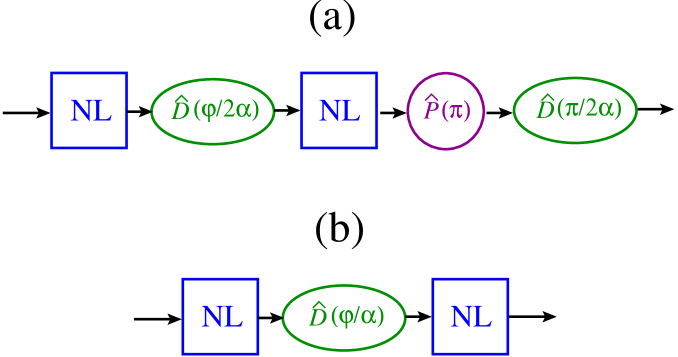
Figure 4: (a) A schematic of an approximate qubit rotation $\hat{R}(\varphi)$ using Kerr nonlinearities (NL), displacement operations ($\hat{D}$) and a phase shifter ($\hat{P}$). (b) Another example, $\hat{V}^{\prime}(\varphi)$, which is an approximation of the ideal qubit rotation $\hat{R}^{\prime}(\varphi)$. See text for details.

It turns out that in order to observe the Bell violation it is sufficient for Alice and Bob to implement the operation $\hat{V}(\varphi,\alpha)$

$$\hat{V}(\varphi,\alpha)=\hat{U}_{NL}\hat{D}\left(\frac{i\varphi}{\alpha}\right)\hat{U}_{NL},$$ (19)

which is depicted in Fig. 4(b). The operation $\hat{V}(\varphi,\alpha)$ is an approximation of the ideal rotation $\hat{R}^{\prime}(\varphi)$

$$\hat{R}^{\prime}(\varphi)|\alpha\rangle=\sin 2\varphi|\alpha\rangle+\cos 2\varphi|-\alpha\rangle,$$ (20)

$$\hat{R}^{\prime}(\varphi)|-\alpha\rangle=\cos 2\varphi|\alpha\rangle-\sin 2\varphi|-\alpha\rangle,$$

which results in the same Bell inequality violations as with $\hat{R}(\varphi)$ in Eq. (3). Of course, when $\alpha$ is small, the “real” operation $\hat{V}(\varphi,\alpha)$ is not a good approximation of $\hat{R}^{\prime}(\varphi)$ because the displacement operator is not a good approximation of $\hat{U}_{z}(\varphi)$ in this limit. It is straightforward to calculate that

$$\hat{V}(\varphi,\alpha)|\alpha\rangle=\frac{1}{2}\left\{e^{i\varphi}\Big{(}|\alpha+\frac{i\varphi}{\alpha}\rangle+i|-\alpha-\frac{i\varphi}{\alpha}\rangle\Big{)}\right.$$

$$~{}~{}~{}~{}~{}~{}~{}~{}~{}+\left.ie^{-i\varphi}\Big{(}|-\alpha+\frac{i\varphi}{\alpha}\rangle+i|\alpha-\frac{i\varphi}{\alpha}\rangle\Big{)}\right\},$$

$$\hat{V}(\varphi,\alpha)|-\alpha\rangle=\frac{1}{2}\left\{ie^{i\varphi}\Big{(}|\alpha+\frac{i\varphi}{\alpha}\rangle+i|-\alpha-\frac{i\varphi}{\alpha}\rangle\Big{)}\right.$$

$$~{}~{}~{}~{}~{}~{}~{}~{}~{}+\left.e^{-i\varphi}\Big{(}|-\alpha+\frac{i\varphi}{\alpha}\rangle+i|\alpha-\frac{i\varphi}{\alpha}\rangle\Big{)}\right\}.$$ (21)

If Alice and Bob perform the local operations, $\hat{V}(\phi,\alpha)$ and $\hat{V}(\theta,\alpha)$, on their modes of $|\Phi_{+}\rangle_{AB}$ respectively, the ECS is transformed to $|\Psi^{V}\rangle_{AB}$ as

$$|\Psi^{V}\rangle_{AB} = \frac{N}{2}\left\{e^{i(\phi-\theta)}(-|\beta_{\phi},\gamma_{\theta}\rangle+i|\beta_{\phi},-\gamma_{\theta}\rangle\right.$$ (22)

$$-\left.i|-\beta_{\phi},\gamma_{\theta}\rangle-|-\beta_{\phi},-\gamma_{\theta}\rangle)\right.$$

$$+\left.e^{-i(\phi-\theta)}(-|\gamma_{\phi},\beta_{\theta}\rangle-i|\gamma_{\phi},-\beta_{\theta}\rangle\right.$$

$$+\left.i|-\gamma_{\phi},\beta_{\theta}\rangle-|-\gamma_{\phi},-\beta_{\theta}\rangle)\right\},$$

where $\beta_{\phi,\theta}=\alpha+i\varphi_{\phi,\theta}/\alpha$, $\gamma_{\phi,\theta}=\alpha-i\varphi_{\phi,\theta}/\alpha$. The Bell parameter $S$ in Eq. (8) can then be obtained using the Wigner representation of Eq. (22), as described in the previous section.

Figure 5: The numerically optimized Bell parameter $|S|$ for an ECS with amplitude $\alpha$ using the real local operation (solid curve) and the ideal local operation (dashed curve). See text for details.

The explicit expressions of the Wigner function of state $|\Psi^{V}\rangle_{AB}$ and its Bell parameter $S$ are inappropriate to present here since they are too lengthy. In Fig. 5, we have plotted the absolute Bell parameter $|S|$ of the ECS maximized using the method of steepest descent nume (solid curve) and compare it with the case using the “ideal” rotation (dashed curve). The violations reach up to Cirel’son’s bound $2\sqrt{2}$, as $\alpha$ grows. Remarkably, the Bell violations of the ECS using the “real” operation $\hat{V}(\varphi_{a},\alpha)$ does not require very large values of $\alpha$. The Bell inequality is violated for $\alpha\geq 0.842$ using $\hat{V}(\varphi_{a},\alpha)$ while it was $\alpha\geq 0.723$ when the unphysical idealized local operation $\hat{R}(\varphi)$ was applied. In the case of an ECS with $\alpha=1$ the maximum violation is $S\approx 2.29$ at $\theta_{1}\approx-0.066$, $\theta_{2}\approx 0.066$ $\phi_{1}\approx 0.236$, $\phi_{2}\approx-0.236$.

IV Conclusion

In this paper we have studied the Bell-CHSH inequality with ECSs, local non-linear operations and homodyne measurements. An ECS with a large amplitude is a state which contains quantum correlations between macroscopically distinguishable states. Optical states are considered macroscopically distinguishable if they can be distinguished by homodyne detection. We have shown that the Bell-CHSH inequality can be violated with ECSs using homodyne measurements up to Tsirelson’s bound $2\sqrt{2}$. The bound is approached when $\alpha\gg 1$. Surprisingly, violation of local reality with respect to homodyne measurements persists down to $\alpha\geq 0.842$.

Given the importance of entanglement from both a fundamental perspective and that of applications such as quantum computing, it would be of considerable interest to test these ideas experimentally. In order to generate an ECS with $\alpha=1$ a single mode SCS with amplitude $\alpha=\sqrt{2}\approx 1.414$ is required. For this ECS a maximum value of the Bell parameter is $\approx 2.29$ which is significantly larger than the classical limit. Production of ECSs of this size are within reach of current technology g-1 ; g-15 ; MP ; g-2 . It is known that a SCS with a small amplitude is very well approximated by a squeezed single photon g-1 . A SCS with amplitude $\sqrt{2}$ and fidelity $\approx 0.97$ may be produced by squeezing a single photon with 4.8dB squeezing, which is experimentally feasible.

The strength of the Kerr non-linearity required for the local operations remains challenging however, efforts are being made to obtain nonlinear effects of sufficient strength using electromagnetically induced transparency Hau ; MP ; Pet . It should be noted that ECSs with small amplitudes, which we are interested in for experimental realization, are relatively less sensitive to noise during the nonlinear interactions.

The experimental realization of Bell violations with large amplitudes, $\alpha\gg 1$, would be even more interesting since in this limit, ECSs can be considered to be truly “macroscopic” entanglement. As shown in Fig. 5, Bell inequality violations close to the Cirel’son’s bound occur for $\alpha\gg 1$. There are some technical difficulties in approaching this regime experimentally. Firstly, it is known that the generation of an ECS of an amplitude $\alpha\gg 1$ is experimentally more demanding. However, some recent theoretical proposals are expected to be experimentally implemented in foreseeable future to generate ECSs with large amplitudes. For example, one may use the SCS amplification scheme g-1 , which uses beam splitters, ancillary coherent states and photodetectors, to distill large SCSs out of small ones. It was shown that a SCS of $\alpha\approx 2.5$, which means an ECS of $\alpha\approx 1.8$ may be realized using experimentally available resources with a high fidelity g-1 . Secondly, in the case of a large $\alpha$, the local operations will be harder to be performed. When amplitudes of ECSs are larger, they suffer more rapid destruction of quantum coherence in the nonlinear media used for the local operations. Methods to efficiently perform the local operations for our Bell inequality tests deserve further investigations.

- (1) J. S. Bell, Physics 1, 195 (1964).
- (2) E. Schrdinger, Naturwissenschaften 23, pp. 807-812; 823-828; 844-849 (1935); K. E. Cahill and R. J. Glauber, Phys. Rev. 177, 1857 (1969).
- (3) B. C. Sanders, Phys. Rev. A45, 6811 (1992); B. C. Sanders, K. S. Lee, and M. S. Kim, Phys. Rev. A52, 735 (1995).
- (4) P. T. Cochrane, G. J. Milburn, and W. J. Munro, Phys. Rev. A59, 2631 (1999).
- (5) S. J. van Enk and O. Hirota, Phys. Rev. A64, 022313 (2001).
- (6) H. Jeong, M. S. Kim, and J. Lee, Phys. Rev. A64, 052308 (2001).
- (7) X. Wang, Phys. Rev. A64, 022302 (2001).
- (8) H. Jeong and M. S. Kim, Phys. Rev. A65, 042305 (2002).
- (9) T. C. Ralph, W. J. Munro, and G. J. Milburn, Proceedings of SPIE 4917, 1 (2002); T. C. Ralph, A. Gilchrist, G. J. Milburn, W. J. Munro, and S. Glancy, Phys. Rev. A68, 042319-1 (2003).
- (10) Nguyen Ba An, Phys. Rev. A68, 022321 (2003); Nguyen Ba An, Phys. Rev. A69, 022315 (2004).
- (11) H. Jeong and M. S. Kim, Quantum Information and Computation 2, 208 (2002).
- (12) J. Clausen, L. Knöll, and D. G. Welsch, Phys. Rev. A66, 062303 (2002).
- (13) S. Glancy, H. M. Vasconcelos, and T. C. Ralph, Phys. Rev. A70, 022317 (2004).
- (14) A. P. Lund, H. Jeong, T. C. Ralph, and M. S. Kim, Phys. Rev. A70, 020101(R) (2004); H. Jeong, A. P. Lund, and T. C. Ralph, Phys. Rev. A72, 013801 (2005).
- (15) H. Jeong, M. S. Kim, T. C. Ralph, and B. S. Ham, Phys. Rev. A70, 061801(R) (2004).
- (16) M. Paternostro, M. S. Kim, and B. S. Ham, Phys. Rev. A67, 023811 (2003); J. Mod. Opt. 50, 2565 (2003).
- (17) J. Wenger, R. Tualle-Brouri, Ph. Grangier, Phys. Rev. Lett. 92, 153601 (2004); J. Wenger, R. Tualle-Brouri, and Ph. Grangier, Phys. Rev. Lett. 92, 153601 (2004); J. S. Neergaard-Nielsen, B. M. Nielsen, C. Hettich, K. Molmer, and E. S. Polzik, quant-ph/0602198; A. Ourjoumtsev, R. Tualle-Brouri, J. Laurat, and Ph. Grangier, Science 312, 83 (2006).
- (18) D. Wilson, H. Jeong, and M. S. Kim, J. Mod. Opt. 49, Special issue for QEP 15, 851 (2002).
- (19) H. Jeong, W. Son, M. S. Kim, D. Ahn, C. Brǔkner, Phys. Rev. A67, 012106 (2003).
- (20) A. Gilchrist, P. Deuar, and M. D. Reid, Phys. Rev. Lett. 80, 3169 (1998); H. Nha and H. J. Carmichael, Phys. Rev. Lett. 93, 020401 (2004); R. García-Patrón, J. Fiurášek, N. J. Cerf, J. Wenger, R. Tualle-Brouri, and Ph. Grangier, Phys. Rev. Lett. 93, 130409 (2004).
- (21) J. F. Clauser, M. A. Horne, A. Shimony, and R. A. Holt, Phys. Rev. Lett. 23, 880 (1969).
- (22) B. S. Tsirelson, Lett. Math. Phys. 4, 93 (1980).
- (23) R. García-Patrón, J. Fiurášek, N. J. Cerf, J. Wenger, R. Tualle-Brouri, and Ph. Grangier, Phys. Rev. Lett. 93, 130409-1 (2004).
- (24) The error rate for discriminating between two coherent states, and , can be calculated as .
- (25) W. H. Pres, B. P. Flannery, S. A. Teukolsky, and W. T. Vetterling, Numerical Recipes (Cambridge University Press, Cambridge, 1988).
- (26) B. Yurke and D. Stoler, Phys. Rev. Lett. 57, 13 (1986).
- (27) L. V. Hau, S. E. Harris, Z. Dutton, and C. H. Behroozi, Nature 397, 594 (1999).
- (28) D. Petrosyan and G. Kurizki, Phys. Rev. A65, 33833 (2002).