Structure of the photon and magnetic field induced birefringence and dichroism

Abstract

In this letter we show that the dichroism and ellipticity induced on a linear polarized light beam by the presence of a magnetic field in vacuum can be explained in the framework of the de Broglie’s fusion model of a photon. In this model it is assumed that the usual photon is the spin 1 state of a particle-antiparticle bound state of two spin 1/2 fermions. The other $S=0$ state is referred to as the second photon. On the other hand, since no charged particle neither particles having an electric dipole are considered, no effect is predicted in the presence of electric fields and this model is not in contradiction with star cooling data or solar axion search.

Very recently an experimental observation of optical activity of vacuum in the presence of a magnetic field has been reported Zavattini:06 by the PVLAS collaboration. The observed results could not be explained in the framework of the standard Quantum ElectroDynamics (QED), and the existence of light pseudoscalar spinless bosons of the same nature of the Peccei and Quinn axion Peccei:77 has been suggested (see e.g. Lamoreaux:06 ). This explanation however is in contradiction with other existing experimental data. In particular, the particle needed to justify the PVLAS results should be largely produced in the star core by interaction of photons with plasma electric fields. Such a particle should escape because of its very low coupling with matter, and induce a fast cooling of stars at a level already excluded by astrophysical observationsRaffelt:96 . Moreover, CAST experiment Zioutas:05 devoted to detect solar axions by conversion in a magnetic field, has already excluded the existence of such a particle in the range of mass and coupling constant necessary to give the PVLAS effect. To get rid of this contradiction more exotic solutions have been proposed. In particular, the existence of a massive paraphoton which would couple with the standard photon Masso:06 and with the axionlike particle (ALP), the photon-initiated real or virtual production of pair of low mass millicharged particles Gies:06 , and the existence of an ultralight pseudo-scalar particle interacting with two photons and a scalar boson and the existence of a low scale phase transition in the theory Mohapatra:07 .

In this letter we show that dichroism and ellipticity induced on a linear polarized light beam by the presence of a magnetic field in vacuum can be predicted in the framework of the de Broglie’s fusion model of a photon Broglie:32 . In this model it is assumed that the usual photon is the spin 1 state of a particle-antiparticle bound state of two spin 1/2 fermions. The other $S=0$ state is referred to as the second photon. The mass of the usual photon is supposed to be zero or negligible.

In particular, we show that taken the spin-spin coupling and the interaction with an external magnetic field proportional to ${\mbox{\boldmath$s$}}_{1}.{\mbox{\boldmath$s$}}_{2}$ and ${\mbox{\boldmath$B$}}.({{\mbox{\boldmath$s$}}_{1}}-{{\mbox{\boldmath$s$}}_{2}})$, respectively, magnetic induced birefringence and dichroism are obtained with a $(\mbox{\boldmath$\epsilon$}.{\mbox{\boldmath$B$}})^{2}$ pseudo-scalar symmetry where $\epsilon$ is the polarization of the photon (as usual $\epsilon$ is defined by the direction of the electric field). Thus both dephasing and absorption appear for linearly polarized light parallel to the external applied magnetic field.

On the other hand, since no charged particle neither particles having an electric dipole are considered, no effect is predicted in the presence of electric fields and this model is not in contradiction with star cooling data or solar axion search.

We consider the photon as composed of a spin 1/2 particle and its antiparticle. The spin Hamiltonian is assumed to be approximate by

$$H_{0}=-\frac{\Delta}{\hbar^{2}}\,{\mbox{\boldmath$s$}}_{1}.{\mbox{\boldmath$s$}}_{2}$$ (1)

with $\Delta>0$. The ground state eigenstates are then given by:

$$|{S\mbox{=}1,M_{z}\mbox{=}1}\rangle = |{\uparrow,\uparrow}\rangle;\quad|{S\mbox{=}1,M_{z}\mbox{=}-1}\rangle=|{\downarrow,\downarrow}\rangle$$

$$|{S\mbox{=}1,M_{z}\mbox{=}0}\rangle = \frac{1}{\sqrt{2}}\,\Big{(}|{\uparrow,\downarrow}\rangle+|{\downarrow,\uparrow}\rangle\Big{)}$$ (2)

with energy $E_{1}=-\Delta/4$, corresponding to the ordinary photon $\gamma_{1}$. The second photon $\gamma_{0}$ is then given by the excited singlet state

$$|{S\mbox{=}0,M_{z}\mbox{=}0}\rangle=\frac{1}{\sqrt{2}}\,\Big{(}|{\uparrow,\downarrow}\rangle-|{\downarrow,\uparrow}\rangle\Big{)}$$ (3)

with energy $E_{0}=(3/4)\,\Delta$. The energy difference between the two photons $\gamma_{1}$ and $\gamma_{0}$ is then given by $\Delta$.

We assume the particle/antiparticle have magnetic moments $\mbox{\boldmath$m$}_{1}=(\beta\,\mu_{B}/\hbar)\,{\mbox{\boldmath$s$}}_{1}$ and $\mbox{\boldmath$m$}_{2}=-\mbox{\boldmath$\mu$}_{1}$. Thus the total magnetic moment ${\mbox{\boldmath$m$}}=(\beta\,\mu_{B}/\hbar)\,({\mbox{\boldmath$s$}}_{1}-{\mbox{\boldmath$s$}}_{2})$ has zero average value for the $\gamma_{1}$ photon and ${m}_{z}=\beta\,\mu_{B}$ for the $\gamma_{0}$ photon.

In the presence of a magnetic field $\bf B$ along $Oz$ we shall have

$$V=(\beta\,\mu_{B}\,B/\hbar)\,({{\mbox{\boldmath$s$}}_{1}}_{z}-{{\mbox{\boldmath$s$}}_{2}}_{z})$$ (4)

The only non-zero matrix element of $V$ is

$$\langle{S\mbox{=}1,M_{z}\mbox{=}0}|{V}|{S\mbox{=}0,M_{z}\mbox{=}0}\rangle=\beta\,\mu_{B}\,B$$ (5)

After diagonalisation $\displaystyle|{\Psi_{1,0}}\rangle$ $\displaystyle=$ $\displaystyle\mbox{cos}\theta\,|{S\mbox{=}1,M_{z}\mbox{=}0}\rangle+\mbox{sin}\theta\,|{S\mbox{=}0,M_{z}\mbox{=}0}\rangle$ $\displaystyle|{\Psi_{0,0}}\rangle$ $\displaystyle=$ $\displaystyle-\mbox{sin}\theta\,|{S\mbox{=}1,M_{z}\mbox{=}0}\rangle+\mbox{cos}\theta\,|{S\mbox{=}0,M_{z}\mbox{=}0}\rangle$

with

$$\tan(2\,\theta)=2\beta\,\mu_{B}\,B/\Delta$$ (7)

and eigenvalues $\displaystyle\overline{E}_{1}$ $\displaystyle=$ $\displaystyle\frac{E_{1}+E_{0}}{2}-\frac{\Delta}{2}\,\sqrt{1+\tan^{2}(2\,\theta)}$ $\displaystyle\overline{E}_{0}$ $\displaystyle=$ $\displaystyle\frac{E_{1}+E_{0}}{2}+\frac{\Delta}{2}\,\sqrt{1+\tan^{2}(2\,\theta)}$ with the new energy difference

$$\overline{\Delta}=\Delta\,\sqrt{1+\tan^{2}(2\,\theta)}$$ (9)

The ordinary photon $\gamma_{1}$ can be described by a linear combination of the two helicity states $|{S\mbox{=}1,M_{{\mbox{\boldmath$k$}}}\mbox{=}\pm 1}\rangle$ where $M_{{\mbox{\boldmath$k$}}}$ is the projection of the spin angular momentum in the direction of propagation of the photon. Let first note that if the $\gamma_{1}$ is propagating along the direction of the magnetic field, only $|{S\mbox{=}1,M_{z}\mbox{=}\pm 1}\rangle$ will be involved and no effect is expected. Consider now a $\gamma_{1}$ propagating along $Oy$ and linearly polarized in the direction of $Oz$. We shall have

$$|{\epsilon_{z}}\rangle=-\frac{1}{\sqrt{2}}\,\Big{(}|{S\mbox{=}1,M_{y}\mbox{=}1}\rangle-|{S\mbox{=}1,M_{y}\mbox{=}-1}\rangle\Big{)}$$ (10)

but

$$|{S,M_{y}}\rangle=\sum_{M_{z}\mbox{=}0,\pm 1}\,|{S,M_{z}}\rangle\,d^{S}_{M_{z},M_{y}}(\pi/2)$$ (11)

where the $d^{S}_{M_{z},M_{y}}$ are the Wigner $d$-functions. Using $\displaystyle d^{1}_{1,\pm 1}(\Theta)$ $\displaystyle=$ $\displaystyle\frac{1}{2}(1\pm\cos\Theta)$ $\displaystyle d^{1}_{0,\pm 1}(\Theta)$ $\displaystyle=$ $\displaystyle\pm\frac{1}{2}\,\sqrt{2}\,\sin\Theta$ $\displaystyle d^{1}_{-1,\pm 1}(\Theta)$ $\displaystyle=$ $\displaystyle\frac{1}{2}(1\mp\cos\Theta)$

we get from (10) and (11)

$$|{\epsilon_{z}}\rangle=-|{S\mbox{=}1,M_{z}\mbox{=}0}\rangle$$ (13)

and this state will be affected by the magnetic field through its coupling to the $|{S\mbox{=}0,M_{z}\mbox{=}0}\rangle$ state. We note in passing that in the case of a linear polarization along the $Ox$ axis we have

$$|{\epsilon_{y}}\rangle = \frac{1}{\sqrt{2}}\,\Big{(}|{S\mbox{=}1,M_{y}\mbox{=}1}\rangle+i\,|{S\mbox{=}1,M_{y}\mbox{=}-1}\rangle\Big{)}$$ (14)

$$= \frac{1}{\sqrt{2}}\,\Big{(}|{S\mbox{=}1,M_{z}\mbox{=}1}\rangle+i\,|{S\mbox{=}1,M_{z}\mbox{=}-1}\rangle\Big{)}$$

and this state will not be affected by the magnetic field.

We assume that the magnetic field is switch-on between $t=0$ and $t=\tau=L/c$, where $L$ is the field length (of the order of 1 m in PVLAS experiment). We shall have $|{\psi(0)}\rangle=-|{1,0}\rangle=-\cos\theta\,|{\Psi_{1,0}}\rangle+\sin\theta\,|{\Psi_{0,0}}\rangle$ where from now on the kets correspond to $|{S,M_{z}}\rangle$. At time $\tau$

$$|{\psi(\tau)}\rangle = -\cos\theta\,e^{-i\,\overline{E}_{1}\,\tau/\hbar}\,|{\Psi_{1,0}}\rangle$$ (15)

$$+ \sin\theta\,e^{-i\,\overline{E}_{0}\,\tau/\hbar}\,|{\Psi_{0,0}}\rangle$$ (16)

which in terms of the non-perturbed kets $|{1,0}\rangle$ and $|{0,0}\rangle$, will be given by

$$|{\psi(\tau)}\rangle = -\left(\cos^{2}\theta\,e^{-i\,\overline{E}_{1}\,\tau/\hbar}+\sin^{2}\theta\,e^{-i\,\overline{E}_{0}\,\tau/\hbar}\right)\,{|{1,0}\rangle}$$ (17)

$$- \cos\theta\,\sin\theta\,\left(e^{-i\,\overline{E}_{1}\,t/\hbar}-e^{-i\,\overline{E}_{0}\,\tau/\hbar}\right)\,{|{0,0}\rangle}$$

This can be written as

$$|{\psi(\tau)}\rangle = -e^{-i\,(E_{1}+E_{0})\,\tau/2\hbar}\,\Bigg{[}\Big{(}\cos(\overline{\Delta}\,\tau/2\hbar)$$ (18)

$$+ i\cos(2\theta)\,\sin(\overline{\Delta}\,\tau/2\hbar)\Big{)}\,{|{1,0}\rangle}$$

$$+ i\,\sin(2\theta)\,\sin(\overline{\Delta}\,\tau/2\hbar)\,{|{0,0}\rangle}\Bigg{]}$$

From (18) the probability to produce $|{0,0}\rangle$ is $P_{\gamma_{1}\to\gamma_{0}}=|\langle 0,0|{\psi(\tau)}\rangle|^{2}$ which gives

$$P_{\gamma_{1}\to\gamma_{0}}=\frac{\tan^{2}(2\theta)}{1+\tan^{2}(2\theta)}\,\sin^{2}\Big{(}{\Delta}\,\sqrt{1+\tan^{2}(2\theta)}\,\tau/2\hbar\Big{)}$$ (19)

with $\tan^{2}(2\theta)$ given by (7).

In the limit where $2\beta\,\mu_{B}\,B\ll\Delta$, $\tan^{2}(2\theta)\ll 1$, and

$$P_{\gamma_{1}\to\gamma_{0}}\simeq\left(\frac{\beta\,\mu_{B}\,B\,\tau}{\hbar}\right)^{2}\,\left(\frac{\sin\Big{(}\Delta\,\tau/2\hbar\Big{)}}{\Delta\,\tau/2\hbar}\right)^{2}$$ (20)

Thus, when $\Delta\,\tau/2\hbar\ll 1$, $P_{\gamma_{1}\to\gamma_{0}}$ does not depend on $\Delta$.

In an apparatus like the PVLAS one where a linearly polarized laser passes through a region where a magnetic field pointing at 45 degrees with respect to light polarization plane is present, such a conversion probability will show as a linear dichroism giving an apparent rotation of the polarization plane $\rho=\frac{1}{2}P_{\gamma_{1}\to\gamma_{0}}$. It is worth to stress that standard QED Adler:71 does not predict any dichroism for light propagating in vacuum in the presence of a magnetic field.

As for the phase of the $|{1,0}\rangle$, this is given by

$$\overline{\phi}_{1}=-(E_{1}+E_{0})\,\tau/2\hbar+\arctan\left[\cos(2\theta)\,\tan(\overline{\Delta}\,\tau/2\hbar)\right]$$ (21)

On the other hand, for the $Ox$ polarization the phase is $\phi_{1}=E_{1}\,\tau/\hbar$. The phase difference between $\gamma_{1}$ states for polarization along and perpendicular to the magnetic field is then given by

$$\delta\phi\equiv\overline{\phi}_{1}-{\phi}_{1}=\arctan\left[\cos(2\theta)\,\tan(\overline{\Delta}\,\tau/2\hbar)\right]-{\Delta}\,\tau/2\hbar$$ (22)

Expanding this function in powers of $\theta$ around zero, we found

$$\delta\phi=\left(\frac{\beta\,\mu_{B}\,B}{\Delta}\right)^{2}\,\left(\frac{\Delta\,\tau}{\hbar}-\sin({\Delta}\,\tau/\hbar)\right)$$ (23)

Again, in the case of an apparatus like the PVLAS one, this dephasing will show as an ellipticity $\epsilon=\delta\phi/2$ acquired by the polarized beam passing through the magnetic field region. Ellipticity is associated to the existence of a birefringence by the formula

$$\epsilon=\frac{\pi\,L}{\lambda}(n_{\|}-n_{\bot})$$ (24)

where $\lambda$ is the light wavelength, and $n_{\|}$ and $n_{\bot}$ are the indexes of refraction for light polarized parallel and perpendicular with respect to the magnetic field, respectively. Thus, in the framework of our model a vacuum will show an apparent magnetic birefringence

$$(n_{\|}-n_{\bot})=\left(\frac{\lambda}{2\pi\,c\,\tau}\right)\left(\frac{\beta\,\mu_{B}\,B}{\Delta}\right)^{2}\,\left(\frac{\Delta\,\tau}{\hbar}-\sin({\Delta}\,\tau/\hbar)\right)$$ (25)

that depends on the time the photon stays in the magnetic field region. Standard QED predicts that a vacuum is a magnetic birefringent medium showing a $(n_{\|}-n_{\bot})\simeq 4\times 10^{-24}B^{2}$ where $B$ is given in Tesla. That only depends on the value of fundamental constants and the square of the magnetic field intensity Adler:71 . QED also predicts that a corresponding effect exists in the presence of an electric field, such an effect is absent in the framework of our model.

We note that our formulas for the conversion probability and the dephasing are equivalent to the ones obtained in the axion case Maiani:86 since axion-photon coupling can be also treated as a two level system Raffelt:88 . Our $\Delta$ corresponds to the ratio ${m_{a}^{2}}/{\omega}$ and $\beta$ to $g_{a\gamma\gamma}$, where $m_{a}$ is the axion mass, $\omega$ the photon energy, and $g_{a\gamma\gamma}$ the axion-photon coupling constant. The mass and coupling constant associated to the ALP needed to explain PVLAS results, $m_{a}\approx 10^{-3}$ eV and $g_{a\gamma\gamma}\approx 3\times 10^{-6}$ GeV^-1 Zavattini:06 , have been chosen by comparing the dichroism signal of PVLAS with limits published by the BRFT collaboration in 1993 Cameron:93 . In fig. 1 we show the corresponding graph following equation (20). We have assumed as usual that the measured effect is simply the effect predicted by this formula multiplied by the number of passages in the magnetic field due of the presence of optical cavities. Dotted line represents the lower border of the parameters plane forbidden by BRFT results at a 2$\sigma$ level, while full line represents the PVLAS signal.

The main difference between our model and the axion model is that in our case the optical effects do not depend on the photon energy. Thus, in our case, the oscillations between the two states of the hamiltonian only depend on the time the $\gamma_{1}$ stay in the magnetic field i.e. the length of the magnetic field region. In the axion case the oscillations depend on the length divided by the photon energy $\omega$. Oscillations can therefore be avoided by choosing higher energy photons for longer magnets, and that was the case of BRFT collaboration with respect to PVLAS collaboration. Eventually, this explains why in our case the allowed window for the parameters that could explain the PVLAS dichroism is larger that in the axion case treated in ref. Zavattini:06 .

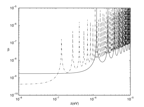
Figure 1: Comparison between PVLAS signal and BRFT limits

In our model the mixing between the ordinary photon $\gamma_{1}$ and the second photon $\gamma_{0}$ only appears in a magnetic field. This will not affect the energy balance and star evolution, but should be important in the case of photon emission from neutron stars which show magnetic fields as high as $10^{9}$ T. This is anyway an important issue also for ALP (see e.g. ref. Dupays:05 , and Lai:06 ).

Since the fusion model assumes structure of the photon, we should expect excited states associated to internal motion and presumably non zero mass of the constituents. However, if the masses and the spatial dimension of the photon are very small, the first excited state can be very high up in energy.

In conclusion, once the PVLAS signal will be confirmed, the exotic but simple de Broglie’s fusion model for the photon can provide an explanation for this signal that is not in contradiction with star observation or solar axion search. On the other hand, experiments testing the propagation of light in the presence of a magnetic field in terrestrial laboratories or by astrophysical observations can put more and more stringent limits on its free parameters.

I Acknowledgements

We thanks E. Massó for very helpful discussion and carefully reading our manuscript.

References

- (1) E. Zavattini et al., Phys. Rev. Lett. 96, 110406 (2006).
- (2) R. D. Peccei and H. R. Quinn, Phys. Rev. Lett. 38, 1440 (1997).
- (3) S. Lamoreaux, Nature 441, 31 (2006).
- (4) G. G. Raffelt, Stars as Laboratories for Fundamental Physics (University of Chicago Press, Chicago, 1996).
- (5) K. Zioutas et al., Phys. Rev. Lett. 94, 121301 (2005).
- (6) E. Masso and J. Redondo, Phys. Rev. Lett. 97, 151802 (2006).
- (7) H. Gies, J. Jaeckel and A. Ringwald, Phys. Rev. Lett. 97, 140402 (2006).
- (8) R. N. Mohapatra and Salah Nasri, Phys. Rev. Lett. 98, 050402 (2007).
- (9) L. de Broglie, C. R. Acad. Sci. Paris 195, 536 (1932); 195, 577 (1932); 197, 1377 (1933); 198, 135 (1934).
- (10) S. L. Adler, Ann. Phys. (NY) 67, 599 (1971).
- (11) L. Maiani, R. Petronzio and E. Zavattini, Phys. Lett. B 175, 359 (1986).
- (12) G. Raffelt and L. Stodosky, Phys. Rev. D 37, 1237 (1988).
- (13) R. Cameron et al., Phys. Rev. D 47, 3707 (1993).
- (14) A. Dupays, C. Rizzo, M. Rocandelli, and G.F. Bignani Phys. Rev. Lett. 95, 211302 (2005).
- (15) D. Lai and J Heyl, Phys. Rev. D 74, 123003 (2006).