Monogamy Inequality in terms of Negativity for Three-Qubit States

Abstract

We propose a new entanglement measure to quantify three qubits entanglement in terms of negativity. A monogamy inequality analogous to Coffman-Kundu-Wootters (CKW) inequality is established. This consequently leads to a definition of residual entanglement, which is referred to as three-$\pi$ in order to distinguish from three-tangle. The three-$\pi$ is proved to be a natural entanglement measure. By contrast to the three-tangle, it is shown that the three-$\pi$ always gives greater than zero values for pure states belonging to the $W$ and GHZ classes, implying there always exists three-way entanglement for them, and three-tangle generally underestimates three-way entanglement of a given system. This investigation will offer an alternative tool to understand genuine multipartite entanglement.

I Introduction

Quantum entanglement lies at the heart of quantum information processing and quantum computationnielsen , accordingly its quantification has drawn much attention in the last decade. In order for such quantification legitimate measures of entanglement are needed as a first step. The existing well-known bipartite measure of entanglement with an elegant formula is the concurrence derived analytically by Wootterswootters and the entanglement of formationbennett ; hill is a monotonically increasing function of concurrence. They have been applied to describing quantum phase transition in various interacting quantum many-body systemsosterloh ; wu . Another useful entanglement measure is negativitywe , regarded as a quantitative version of Peres’ criterion for separability. Comparing with the concurrence, the process calculating the negativity is significantly simplified with respect to mixed states since it does not need the convex-proof extension.

On the other hand, multipartite entanglement is a valuable physical resource in large-scale quantum information processingbri and plays an important role in condensed matter physics. The negativity is used to study multipartite entanglement in a Fermi gaslunkes . However, it is a formidable task to quantify multipartite entanglement since there is few well-defined multipartite entanglement measures just like for bipartite systems. As for now, the widely-used basis for characterizing and quantifying tripartite entanglement is the three-tangle coffman . Very recently the proof for the general CKW inequality for bipartite entanglementosborne and the demonstration that the CKW inequality cannot generalize to higher-dimensional systemsou1 have been provided.

Recall that the concurrence of a two-qubit state $\rho$ is defined as $\mathcal{C}(\rho)\equiv\max\{0,\sqrt{\lambda_{1}}-\sqrt{\lambda_{2}}-\sqrt{\lambda_{3}}-\sqrt{\lambda_{4}}\}$, in which $\lambda_{1},...,\lambda_{4}$ are the eigenvalues of the matrix $\rho(\sigma_{y}\otimes\sigma_{y})\rho^{*}(\sigma_{y}\otimes\sigma_{y})$ in nonincreasing order and $\sigma_{y}$ is a Pauli spin matrix. For a pure three-qubit state $\rho_{ABC}$, the CKW inequality in terms of concurrence can read

$$\mathcal{C}_{AB}^{2}+\mathcal{C}_{AC}^{2}\leq\mathcal{C}_{A(BC)}^{2},$$ (1)

where $\mathcal{C}_{AB}$ and $\mathcal{C}_{AC}$ are the concurrences of the mixed states $\rho_{AB}=\mathrm{Tr}_{C}(|\phi\rangle_{ABC}\langle\phi|)$ and $\rho_{AC}=\mathrm{Tr}_{B}(|\phi\rangle_{ABC}\langle\phi|)$, respectively, and $\mathcal{C}_{A(BC)}=2\sqrt{\det\rho_{A}}$ with $\rho_{A}=\mathrm{Tr}_{BC}(|\phi\rangle_{ABC}\langle\phi|)$. According to Eq.(1) the three-tangle can be defined as

$$\tau_{ABC}=C_{A(BC)}^{2}-C_{AB}^{2}-C_{AC}^{2},$$ (2)

which is used to characterize three-way entanglement of the statedue . For example, quantified by the three-tangle, the state $|\mathrm{GHZ}\rangle=\frac{1}{\sqrt{2}}(|000\rangle+|111\rangle)$ has only three-way entanglement, while the state $|W\rangle=\frac{1}{\sqrt{3}}(|100\rangle+|010\rangle+|001\rangle)$ has only two-way entanglement. For a general mixed three-qubit state of $\rho_{ABC}$ the three-tangle should be $\tau_{ABC}=\min\left[C_{A(BC)}^{2}\right]-C_{AB}^{2}-C_{AC}^{2}$, where $C_{A(BC)}^{2}$ has to be minimized for all possible decomposition of $\rho_{ABC}$. Now one may wonder whether there exist other entanglement measures satisfying Eq.(1) and whether the three-way entanglement of a given state provided by these entanglement measures is the same. This will help us further understand genuine multipartite entanglement.

To this end, the main result of this paper is to provide a monogamy inequality in terms of negativity. In Sec II, we recall some basic concepts of the negativity. In Sec III, we deduce the monogamy inequality in terms of negativity. In Sec IV and V, the three-$\pi$ analogous to three-tangle is defined, which is shown to be a natural entanglement measure. By calculation on the $|W\rangle$ state, the $|\mathrm{GHZ}\rangle$ state, and the superposed states of the two states, the three-$\pi$ is shown to be greater than zero, i.e., for such states there always exists three-way entanglement. It is also shown that the three-$\pi$ is always not less than the three-tangle for any tripartite pure states and can be extended to mixed three-qubit states and general pure $n$-qubit states. The conclusions are in Sec VI.

II Basic concepts of the negativity

For a either pure or mixed state $\rho$ in the tensor product $\mathcal{H}_{A}\otimes\mathcal{H}_{B}$ of two Hilbert spaces $\mathcal{H}_{A}$, $\mathcal{H}_{B}$ for two subsystems $A$ and $B$, the partial transpose with respect to $A$ subsystem is $(\rho^{T_{A}})_{ij,kl}=(\rho)_{kj,il}$ and the negativity is defined by $\mathcal{N}={(\|\rho^{T_{A}}\|-1})/{2}$ where the trace norm $\|R\|$ is given by $\|R\|=\mathtt{Tr}\sqrt{RR^{\dagger}}$. $\mathcal{N}>0$ is the necessary and sufficient inseparable condition for the $2\otimes 2$ and $2\otimes 3$ bipartite quantum systemsho . In order for any maximally entangled state in $2\otimes 2$ systems to have the negativity one, it can be reexpressed as

$$\mathcal{N}=\|\rho^{T_{A}}\|-1,$$ (3)

with only a change of the constant factor 2. Therefore $\mathcal{N}=1$ for Bell states like $\frac{1}{\sqrt{2}}(|01\rangle+|01\rangle)$ and vanishes for factorized states. For pure two-qubit systems in terms of the coefficients $\{\phi_{00},\phi_{01},\phi_{10},\phi_{11}\}$ of $|\phi_{AB}\rangle$ with respect to an orthonormal basis the concurrence is defined as $\mathcal{C}_{AB}=2|\phi_{00}\phi_{11}-\phi_{01}\phi_{10}|$. From Eq.(3) it is easy to check that $\mathcal{N}_{AB}=\mathcal{C}_{AB}$ for such systems. Now let us consider pure three-qubit systems $A$, $B$, and $C$ in the standard basis $\{|ijk\rangle\}$, where each index takes the values 0 and 1: $|\phi\rangle_{ABC}=\sum_{ijk}\phi_{ijk}|ijk\rangle$. For our goal it is necessary to show $\mathcal{N}_{A(BC)}=\mathcal{C}_{A(BC)}$. The density matrix of $|\phi\rangle_{ABC}$ is $\rho=|\phi\rangle_{ABC}\langle\phi|$ and $\rho^{T_{A}}=\sum_{ijk,i^{\prime}j^{\prime}k^{\prime}}\phi_{ijk}\phi_{i^{\prime}j^{\prime}k^{\prime}}^{\ast}|i^{\prime}jk\rangle\langle ij^{\prime}k^{\prime}|$. Following from Eq.(3) we arrive at

$$\mathcal{N}_{A(BC)} = \|\sum_{ijk,i^{\prime}j^{\prime}k^{\prime}}\phi_{ijk}\phi_{i^{\prime}j^{\prime}k^{\prime}}^{\ast}|i^{\prime}jk\rangle\langle ij^{\prime}k^{\prime}|\|-1$$ (4)

$$= \|\sum_{ijk}\phi_{ijk}|jk\rangle\langle i|\otimes\sum_{i^{\prime}j^{\prime}k^{\prime}}\phi_{i^{\prime}j^{\prime}k^{\prime}}^{\ast}|i^{\prime}\rangle\langle j^{\prime}k^{\prime}|\|-1$$

$$= \|R\otimes R^{{\dagger}}\|-1=\|R\|^{2}-1$$

$$= 2\sqrt{\lambda_{0}\lambda_{1}}=\mathcal{C}_{A(BC)},$$

where $R=\sum_{i^{\prime}j^{\prime}k^{\prime}}\phi_{i^{\prime}j^{\prime}k^{\prime}}^{\ast}|i^{\prime}\rangle\langle j^{\prime}k^{\prime}|$, $\lambda_{0}$ and $\lambda_{1}$ are eigenvalues of $RR^{{\dagger}}$. The obtaining of the third formula is based on the property of the trace norm $\|G\otimes Q\|=\|G\|\cdot\|Q\|$, observation that $RR^{{\dagger}}=\sum_{i^{\prime}j^{\prime}k^{\prime},ijk}\phi_{ijk}\phi_{i^{\prime}j^{\prime}k^{\prime}}^{\ast}|i^{\prime}\rangle\langle j^{\prime}k^{\prime}|\cdot|jk\rangle\langle i|$, and $\|R\|$ is equal to the sum of the square root of eigenvalues $\lambda_{i}$ of $RR^{{\dagger}}$ with $\lambda_{0}+\lambda_{1}=1$. From another observation that $\lambda_{0}$ and $\lambda_{1}$ are also the eigenvalues of the reduced density matrix $\rho_{A}=\mathrm{Tr}_{BC}(|\phi\rangle_{ABC}\langle\phi|)$ whose matrix elements are $\mu_{00}=\sum_{jk}\phi_{0jk}\phi_{0jk}^{\ast},\mu_{01}=\sum_{jk}\phi_{0jk}\phi_{1jk}^{\ast},\mu_{10}=\sum_{jk}\phi_{1jk}\phi_{0jk}^{\ast}$ and $\mu_{11}=\sum_{jk}\phi_{1jk}\phi_{1jk}^{\ast}$, and the concurrence between $A$ and $BC$ is defined as $\mathcal{C}_{A(BC)}=\sqrt{2(1-\mathrm{Tr}\rho_{A}^{2})}=2\sqrt{\lambda_{0}\lambda_{1}}$, the last formula is obtained. The next paragraphs are devoted to one of the main results of this paper.

III Monogamy inequality in terms of negativity

For any pure $2\otimes 2\otimes 2$ states $|\phi\rangle_{ABC}$, the entanglement quantified by the negativity between $A$ and $B$, between $A$ and $C$, and between $A$ and the single object $BC$ satisfies the following CKW- inequality-like monogamy inequality

$$\mathcal{N}^{2}_{AB}+\mathcal{N}_{AC}^{2}\leq\mathcal{N}^{2}_{A(BC)},$$ (5)

where $\mathcal{N}_{AB}$ and $\mathcal{N}_{AC}$ are the negativities of the mixed states $\rho_{AB}=\mathrm{Tr}_{C}(|\phi\rangle_{ABC}\langle\phi|)$ and $\rho_{AC}=\mathrm{Tr}_{B}(|\phi\rangle_{ABC}\langle\phi|)$, respectively.

In order to prove Eq.(5) it is helpful to recall the Theorem appearing inchen , which states that for any $m\otimes n(m\leq n)$ mixed state $\rho$, the concurrence $\mathcal{C}(\rho)$ satisfies

$$\sqrt{\frac{2}{m(m-1)}}(\|\rho^{T_{A}}\|-1)\leq\mathcal{C}(\rho).$$ (6)

In our considered qubit system, $m=n=2$. Therefore it follows from Eqs.(3) and (6) that $\mathcal{N}\leq\mathcal{C}$, implying the negativity is never greater than the concurrence in this case. Thus for the state $|\phi\rangle_{ABC}$ we have

$$\begin{array}[]{ccc}\mathcal{N}_{AB}\leq\mathcal{C}_{AB},&\mathcal{N}_{AC}\leq\mathcal{C}_{AC}.&\end{array}$$ (7)

Observing Eqs.(1), (4) and (7), the conclusion in Eq.(5) can be proved.

In a similar way, if one takes the different focus $B$ and $C$, the following monogamy inequalities

$$\mathcal{N}^{2}_{BA}+\mathcal{N}_{BC}^{2}\leq\mathcal{N}^{2}_{B(AC)},$$ (8)

and

$$\mathcal{N}^{2}_{CA}+\mathcal{N}_{CB}^{2}\leq\mathcal{N}^{2}_{C(AB)},$$ (9)

hold also.

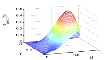
Figure 1: (color online). The three-$\pi$ for the state in Eq.(9) as a function of the coefficients $\beta$ and $\gamma$. Only two coefficients are independent since $|\alpha|^{2}+|\beta|^{2}+|\gamma|^{2}=1$. $\pi_{ABC}(\phi)$ is always greater than zero and reaches maximal value $\frac{4}{9}\left(\sqrt{5}-1\right)$ when $\alpha=\beta=\gamma=\frac{1}{\sqrt{3}}$, which, to a certain degree, demonstrates why the $W$ state is maximally entangled.

Now one naturally would like to care about the tightness of the monogamy inequality in Eq.(5). All pure three-qubit states can be sorted into six classes through stochastic local operation and classical communication(SLOCC)due . (1) $A$–$B$–$C$ class including product states; (2) $A$–$BC$, (3) $B$–$AC$, and (4) $C$–$AB$ classes including bipartite entanglement states; (5) $W$ and (6) GHZ classes including genuine tripartite entanglement states. For the first four classes it is easy to verify that Eqs.(5), (8), and (9) turn out to be an equality, being the same to the CKW inequality. However, it is different for the $W$ class. For the following pure state of $ABC$:

$$|\phi\rangle=\alpha|100\rangle+\beta|010\rangle+\gamma|001\rangle,$$ (10)

which belongs to the $W$ class. Substituting $\mathcal{N}^{2}_{AB}=4\alpha^{2}\beta^{2}+2\gamma^{4}-2\gamma^{2}\sqrt{\gamma^{4}+4\alpha^{2}\beta^{2}}$, $\mathcal{N}^{2}_{AC}=4\alpha^{2}\gamma^{2}+2\beta^{4}-2\beta^{2}\sqrt{\beta^{4}+4\alpha^{2}\gamma^{2}}$, and $\mathcal{N}^{2}_{A(BC)}=4\alpha^{2}(\beta^{2}+\gamma^{2})$ into Eq.(5) we have $\gamma^{4}+\beta^{4}<\gamma^{2}\sqrt{\gamma^{4}+4\alpha^{2}\beta^{2}}+\beta^{2}\sqrt{\beta^{4}+4\alpha^{2}\gamma^{2}}$, resulting in that the inequality in Eq.(5) is strict due to $\alpha\neq 0$, $\beta\neq 0$, and $\gamma\neq 0$, while the CKW inequality can only be an equality for the $W$ classdue .

Having seen that both the equality and inequality in Eq.(5) can be satisfied by some three-qubit states, we can define the residual entanglement, which is referred to as the three-$\pi$ in order to distinguish from the three-tangle in the following main results of this paper.

IV  Three-$\pi$ entanglement measure

The difference between the two sides of Eq.(5) can be interpreted as the residual entanglement

$$\pi_{A}=\mathcal{N}^{2}_{A(BC)}-\mathcal{N}^{2}_{AB}-\mathcal{N}_{AC}^{2}.$$ (11)

Likewise, Eqs.(8) and (9) gives birth to the corresponding residual entanglement as

$$\pi_{B}=\mathcal{N}^{2}_{B(AC)}-\mathcal{N}^{2}_{BA}-\mathcal{N}_{BC}^{2},$$ (12)

and

$$\pi_{C}=\mathcal{N}^{2}_{C(AB)}-\mathcal{N}^{2}_{CA}-\mathcal{N}_{CB}^{2},$$ (13)

respectively. The subscripts $A$, $B$, and $C$ in $\pi_{A}$, $\pi_{B}$, and $\pi_{C}$ mean that qubit $A$, qubit $B$, and qubit $C$ are taken as the focus, respectively. Unlike the three-tangle, in general $\pi_{A}\neq\pi_{B}\neq\pi_{C}$, which can be easily confirmed after calculating them for the state in Eq.(10). This indicates that the residual entanglement corresponding to the different focus is variant under permutations of the qubits. We take $\pi_{ABC}$ (referred to as the three-$\pi$) as the average of $\pi_{A}$, $\pi_{B}$, and $\pi_{C}$, i.e.,

$$\pi_{ABC}=\frac{1}{3}(\pi_{A}+\pi_{B}+\pi_{C}),$$ (14)

which thus becomes invariant under permutations of the qubits since, for example, permutation of qubit $A$ and qubit $B$ accordingly only leads to exchanging $\pi_{A}$ and $\pi_{B}$ with each other in $\pi_{ABC}$.

As we will prove here, the three-$\pi$ in Eq.(14) is a natural entanglement measure satisfying three necessary conditionsve . The first condition is that the three-$\pi$ should be local unitary (LU) invariant. After LU transformations $U_{A}$, $U_{B}$, and $U_{C}$ acted separately on a pure three-qubit state $\rho_{ABC}$, the state can read $\rho^{\prime}_{ABC}=U_{A}\otimes U_{B}\otimes U_{C}\rho_{ABC}U^{{\dagger}}_{A}\otimes U^{{\dagger}}_{B}\otimes U^{{\dagger}}_{C}$. It is necessary to prove that the six squared negativities in Eq.(14) are invariant under the three simultaneous LU transformations. Since $\rho^{\prime}_{A}=\mathrm{Tr}_{BC}\rho^{\prime}_{ABC}=U_{A}\rho_{A}U_{A}^{{\dagger}}$ and $\mathcal{N^{\prime}}_{A(BC)}=\mathcal{C^{\prime}}_{A(BC)}=\sqrt{2(1-\mathrm{Tr\rho^{\prime 2}_{A}})}=\mathcal{N}_{A(BC)}$ , $\mathcal{N}_{A(BC)}$ is LU invariant. Similarly $\mathcal{N}_{B(AC)}$ and $\mathcal{N}_{C(AB)}$ are also LU invariant. While $\rho^{\prime}_{AB}=\mathrm{Tr}_{C}\rho^{\prime}_{ABC}=U_{A}\otimes U_{B}\rho_{AB}U^{{\dagger}}_{A}\otimes U^{{\dagger}}_{B}$, together with the property that the negativity itself is LU invariantpere ; vidal , leads to $\mathcal{N}(\rho^{\prime}_{AB})=\mathcal{N}(\rho_{AB})$. Thus $\mathcal{N}(\rho_{AB})$ is LU invariant, so are $\mathcal{N}(\rho_{BC})$ and $\mathcal{N}(\rho_{AC})$. Now we finish proving the first condition.

Observation of Eqs.(5), (8) and (9) shows that $\pi_{ABC}\geq 0$, thus the second condition is satisfied. Moreover, it is easy to verify that $\pi_{ABC}=0$ for product pure states. $\pi_{ABC}$ is invariant under permutations of the qubits allows us to use proof outlinedue to confirm the third condition. Let us consider local positive operator valued measure (POVM’s) for one qubit only. Let $A_{1}$ and $A_{2}$ be two POVM elements such that $A^{{\dagger}}_{1}A_{1}+A^{{\dagger}}_{2}A_{2}=I$. We can write $A_{i}=U_{i}D_{i}V$, with $U_{i}$ and $V$ being unitary matrices, and $D_{i}$ being diagonal matrices with entries $(a,b)$ and $(\sqrt{1-a^{2}},\sqrt{1-b^{2}})$, respectively. Consider an arbitrary initial state $|\psi\rangle$ of qubit $A$, $B$, and $C$ with $\pi_{ABC}(\psi)$. After the POVM, $|\phi^{\prime}\rangle=A_{i}|\psi\rangle$. Normalizing them gives $|\phi_{i}\rangle=|\phi^{\prime}_{i}\rangle/\sqrt{p_{i}}$ with $p_{i}=\langle\phi^{\prime}_{i}|\phi^{\prime}_{i}\rangle$ and $p_{1}+p_{2}=1$. Therefore $\langle\pi_{ABC}\rangle=p_{1}\pi_{ABC}(\phi_{1})+p_{2}\pi_{ABC}(\phi_{2})$. Taking into account both the fact that $\pi_{ABC}(U_{i}D_{i}V\psi)=\pi_{ABC}(D_{i}V\psi)$ due to its LU invariance and the key fact that three-$\pi$ is also a quartic function of its coefficients in the standard basis which can be seen from the calculation for the state of Eq.(10), we have $\pi_{ABC}(\phi_{1})=\frac{a^{2}b^{2}}{p_{1}^{2}}\pi_{ABC}(\psi)$ and $\pi_{ABC}(\phi_{2})=\frac{(1-a^{2})^{2}(1-b^{2})^{2}}{p_{2}^{2}}\pi_{ABC}(\psi)$. After simple algebra calculations, we obtain $\langle\pi_{ABC}\rangle\leq\pi_{ABC}(\psi)$, thus the third condition that the three-$\pi$ should be an entanglement monotone is satisfied.

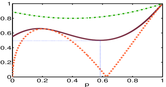
Figure 2: (color online). Plot of $\pi^{(-)}_{ABC}$(solid line), $\tau^{(-)}_{ABC}$(dashed line), and squared $\mathcal{N}^{(-)}_{A(BC)}$ (dashed-dotted line) for the state $|\Psi^{(-)}\rangle_{ABC}$ in Eq.(15) as a function of $p$. The dotted line indicates the minimal value of $\pi^{(-)}_{ABC}$. The two measures match at $p=0.2$ and $p=1$.

V demonstration of two examples and extension to pure multiqubit states

In order to explicitly see the difference between the three-$\pi$ and the three-tangle we present the following two examples.

Example 1: The different classes by SLOCC. For the state in Eq.(10) belonging to the $W$ class we get

$$\pi_{ABC}(\phi) = \frac{4}{3}(\alpha^{2}\sqrt{\alpha^{4}+4\beta^{2}\gamma^{2}}+\beta^{2}\sqrt{\beta^{4}+4\alpha^{2}\gamma^{2}}$$ (15)

$$+\gamma^{2}\sqrt{\gamma^{4}+4\alpha^{2}\beta^{2}}-\alpha^{4}-\beta^{4}-\gamma^{4})$$

$$> \tau_{ABC}(\phi)=0.$$

We also have performed extensive numerical calculation on three-$\pi$ of the other states in the $W$ class and found that it is always greater than zero (i.e., $\pi_{ABC}(W)>0$) as shown in Eq.(15) for the sate $|\phi\rangle$ (see also Fig.1), implying these states have three-way entanglement also. Taking into account that $\tau_{ABC}(W)=0$ a conclusion that the three-tangle underestimates three-way entanglement can be drawn. For the GHZ class we have the property that $\pi_{ABC}(\mathrm{GHZ})=\tau_{ABC}(\mathrm{GHZ})>0$. While $\pi_{ABC}(\mathrm{\Phi})=\tau_{ABC}(\mathrm{\Phi})=0$ for the states $|\Phi\rangle_{ABC}$ belonging to the classes excluding the $W$ and GHZ classes .

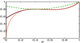
Figure 3: (color online). Plot of $\pi^{(+)}_{ABC}$(solid line), $\tau^{(+)}_{ABC}$(dashed line), and squared $\mathcal{N}^{(+)}_{A(BC)}$ (dashed-dotted line) for the state $|\Psi^{(+)}\rangle_{ABC}$ in Eq.(15) as a function of $p$. The two measures match at $p\in[0.4,1]$, together with squared $\mathcal{N}^{(+)}_{A(BC)}$, they match at $p=0.4$.

Example 2: Superpositions of GHZ and $W$ states. Quantifying of multipartite mixed states is also a fundamental issue in quantum information theory. An optimal decompositions for the three-tangle of mixed three-qubit states composed of a GHZ state and a $W$ state is obtainedlo . In order to further explore the relationship between three-$\pi$ and three-tangle we first write down superposed state of GHZ and $W$ states

$$|\Psi^{(\pm)}\rangle_{ABC}=\sqrt{p}|\mathrm{GHZ}\rangle\pm\sqrt{1-p}|W\rangle.$$ (16)

The three-tangle for $|\Psi^{(\pm)}\rangle_{ABC}$ is known as $\tau^{(\pm)}_{ABC}=|p^{2}\pm\frac{8\sqrt{6}}{9}\sqrt{p(1-p)^{3}}|$ and with Eqs.(11-14) we plot $\pi^{(\pm)}_{ABC}$ (see Fig.2 and 3). The two measures shows similar trend and the fact that $\pi_{ABC}\geq\tau_{ABC}$ is shown. Notice that the similar result was obtained also insh , however, their defined residual entanglement $E=\mathcal{N}_{A(BC)}-\mathcal{N}_{AB}-\mathcal{N}_{AC}$ is not an entanglement measurela . On the other hand, for the state $|\Psi^{(-)}\rangle_{ABC}$ the location of $p$ of the minimal value of the two measures does not match(see Fig.2), i.e., when $p\approx 0.58$ the extremely minimal $\pi^{(-)}_{ABC}\approx 0.5$ which is smaller than $\pi_{ABC}(W)=\frac{4}{9}\left(\sqrt{5}-1\right)\approx 0.55$ being equal to $\pi^{(-)}_{ABC}$ when $p=0$. But $\tau^{(-)}_{ABC}=0$ when $p=\frac{4\sqrt[3]{2}}{3+\sqrt[3]{2}}\approx 0.63$ for the state $|\Psi^{(-)}\rangle_{ABC}$, which provides a basis on the optimal decomposition of mixtures of the GHZ and $W$ stateslo . In a similar way, we can also achieve optimal decomposition of such mixed states for the three-$\pi$ou . Note that for mixed three-qubit states of $ABC$, the monogamy inequality Eq.(5) turns out to be

$$\mathcal{N}^{2}_{AB}+\mathcal{N}_{AC}^{2}\leq\mathrm{min}[\mathcal{N}^{2}_{A(BC)}],$$ (17)

which has to be minimized for all possible decomposition of $\rho_{ABC}$. The other inequalities in Eqs.(8) and (9) need the same manipulations.

Extension to pure multiqubit states. The general CKW inequality for the case of $n$ qubits is provedosborne . Our monogamy inequality can also do this. Denote $n$ qubits by $A_{1},A_{2},...A_{n}$. Eq.(4) may generalize to $\mathcal{N}_{A_{1}(A_{2}A_{3}...A_{n})}=\mathcal{C}_{A_{1}(A_{2}A_{3}...A_{n})}$. Considering the fact that $\mathcal{N}\leq\mathcal{C}$ for mixed two-qubit states and the general CKW inequalityosborne , we prove that

$$\mathcal{N}^{2}_{A_{1}A_{2}}+\mathcal{N}^{2}_{A_{1}A_{3}}+\cdot\cdot\cdot+\mathcal{N}^{2}_{A_{1}A_{n}}\leq\mathcal{N}^{2}_{A_{1}(A_{2}A_{3}...A_{n})},$$ (18)

which may also be used to study the entanglement for a wide class of complex quantum systemsosborne . The general monogamy inequality corresponding to the different focus has a similar form in Eq.(18).

VI Conclusions

Summarizing, we proved a monogamy inequality in terms of negativity such that the three-$\pi$ is defined so as to quantify the residual entanglement for three-qubit states. The three-$\pi$ is shown to be a natural entanglement measure and can be extended to mixed states and general pure $n$-qubit states. The three-way entanglement for the $W$ and GHZ classes quantified by the three-$\pi$ always exists, while the three-tangle is zero for the $W$ class. Compared to the three-$\pi$, the three-tangle generally underestimates the entanglement. Note that the monogamy inequality for distributed Gaussian entanglement in terms of negativity was also establishedadesso and the information-theoretic measure of genuine multiqubit entanglement based on bipartite partitions was introducedzhou . Therefore, further investigation by using the results in this paper will help us deeply understand genuine multipartite entanglement.

References

- (1) M. A. Nielsen and I. L. Chuang, Quantum Computation and Quantum Information (Cambridge University Press, Cambridge, 2000).
- (2) W. K. Wootters, Phys. Rev. Lett. 80, 2245(1998).
- (3) C. H. Bennett, D. P. DiVincenzo, J. A. Smolin, and W. K. Wootters, Phys. Rev. A 54, 3824(1996).
- (4) S. Hill and W. K. Wootters, Phys. Rev. Lett. 78, 5022(1997).
- (5) A. Osterloh, L. Amico, G. Falci, and R. Fazio Nature(London) 416, 608(2002).
- (6) L. A. Wu, M. S. Sarandy, and D. A. Lidar, Phys. Rev. Lett. 93, 250404(2004).
- (7) R. Raussendorf and H. J. Briegel, Phys. Rev. Lett. 86, 5188(2001).
- (8) G. Vidal and R. F. Werner, Phys. Rev. A 65, 032314(2002).
- (9) C. Lunkes, Č. Brukner, and V. Vedral, Phys. Rev. Lett. 95, 030503(2005).
- (10) V. Coffman, J. Kundu, and W. K. Wootters, Phys. Rev. A 61, 052306(2000).
- (11) T. J. Osborne and F. Verstraete, Phys. Rev. Lett. 96, 220503(2006).
- (12) Y. C. Ou, Phys. Rev. A 75, 034305(2007).
- (13) W. Dür, G. Vidal, J. I. Cirac, Phys. Rev. A 62, 062314(2000).
- (14) M. Horodecki, P. Horodecki, and R. Horodecki, Phys. Rev. Lett. 80, 5239(1998).
- (15) K. Chen, S. Albeverio, and S. M. Fei, Phys. Rev. Lett. 95, 040504(2005).
- (16) V. Vedral, M. B. Plenio, M. A. Rippin, and P. L. Knight, Phys. Rev. Lett. 78, 2275(1997).
- (17) A. Peres, Phys. Rev. Lett. 77, 1413(1996).
- (18) G. Vidal and R. F. Werner, Phys. Rev. A 65, 032314(2002).
- (19) R. Lohmayer, A. Osterloh, J. Siewert, and A. Uhlmann, Phys. Rev. Lett. 97, 260502(2006).
- (20) S. S. Sharma and N. K. Sharma, preprint quant-ph/0609012.
- (21) For example, when and for the state in Eq.(10), we get , leading to .
- (22) To appear elsewhere.
- (23) T. Hiroshima, G. Adesso, and F. Illuminati, Phys. Rev. Lett. 98, 050503(2007).
- (24) J. M. Cai, Z. W. Zhou, X. X. Zhou, and G. C. Guo, Phys. Rev. A 74, 042338(2006).