Casimir–Polder forces on excited atoms in the strong atom–field coupling regime

Abstract

Based on macroscopic quantum electrodynamics in linear media, we develop a general theory of the resonant Casimir–Polder force on an excited two-level atom in the presence of arbitrary linear bodies, with special emphasis on the strong-coupling regime where reabsorption of an emitted photon can give rise to (vacuum) Rabi oscillations. We first derive a simple time-independent expression for the force by using a dressed-state approximation. For initially single-quantum excited atom–field systems we then study the dynamics of the force by starting from the Lorentz force and evaluating its average as a function of time. For strong atom–field coupling, we find that the force may undergo damped Rabi oscillations. The damping is due to the decay of both the atomic excitation and the field excitation, and both amplitude and mean value of the oscillations depend on the chosen initial state.

I Introduction

It is well known that the presence of macroscopic bodies can drastically change the properties of the electromagnetic field compared to those observed in free space. A prominent manifestation of the body-induced change of the ground-state fluctuations of the field is the Casimir–Polder (CP) force experienced by an atom when placed within an arrangement of unpolarized ground-state bodies (for a review, see Ref. Buhmann and Welsch (2007)). Originally, CP forces were studied for ground-state atoms where the CP potential can be identified with the position-dependent part of the atom–field coupling energy Casimir and Polder (1948). Since in this case the coupling involves only off-resonant, virtual transitions of the system, the coupling energy can be calculated by means of time-independent leading-order perturbation theory.

For excited systems, on the contrary, real transitions must be taken into account. In particular, when applying the method to an atom in an excited energy eigenstate which interacts with the body-assisted electromagnetic vacuum, one finds that the corresponding CP potential can be significantly enhanced Wylie and Sipe (1985). The enhancement is due to the influence of now possible real transitions to lower states, with the dependence of the force on the atomic transition frequencies exhibiting the typical dispersion profiles in the vicinity of medium resonances. Since these transitions are also responsible for the decay of the atomic excitation, the application of the static approach to the CP force on an excited atom becomes questionable.

Moreover, perturbative methods are known to break down when an atom near-resonantly interacts with a body-assisted narrow-band field such that the strong-coupling regime is realized; this is typically the case when the bodies form a resonatorlike structure. For a two-level atom that (according to the Jaynes–Cummings model Jaynes and Cummings (1963)) is assumed to near-resonantly interact with a single monochromatic mode, it is well known that the energies of the exact excited energy eigenstates of the coupled system—the so-called dressed states—are symmetrically shifted above/below the mean of the unperturbed energy eigenvalues. As the dressed-state energies depend on the atomic position, they can be interpreted as CP potentials Haroche et al. (1991); Englert et al. (1991)—in generalization of the static approach based on leading-order perturbation theory. In particular in the case of a perfect standing wave in a cavity, it turns out that, depending on the upper/lower dressed state the system is prepared in, the atom is repelled from/attracted to the antinodes of the wave—an effect that can strongly affect the motion of the atom Prants and Sirotkin (2001). Calculations imply that atoms sufficiently slowly incident on a cavity in a direction parallel to the standing wave can be reflected from the cavity due to the influence of the upper dressed state Englert et al. (1991); Battocletti and Englert (1994); Bastin and Martin (2003). Here, the dependence of the transmission probability on the velocity of the incident atoms displays a resonance structure Retamal et al. (1998) which may be used to construct a velocity filter for atoms Löffler et al. (1998); Bastin and Martin (2004). In the case of atoms incident in a direction normal to the standing wave, the atoms may be deflected during their passage through the cavity An et al. (2000).

In fact, even if a dressed state was prepared very accurately, the system would not stay in this state forever, but it would undergo a temporal evolution due to unavoidable dissipation, and so would the CP force. To describe the time-dependence of CP forces acting on excited systems, a dynamical approach is required. For weak atom–field coupling, it has been shown that when an initially excited atom exponentially decays to the ground state, the associated CP force shows a similar transient behavior and eventually changes to the ground-state force in the long-time limit Buhmann et al. (2004, 2005); Buhmann and Welsch (2007). A two-level atom which is initially prepared in the upper state and which strongly interacts with a (vacuum) cavity field undergoes Rabi oscillations which are damped due to dissipation; this effect may be phenomenologically incorporated in the Jaynes–Cummings model via damping constants Ren and Carmichael (1995). As simulated in Refs. Doherty et al. (1997, 2000), the losses can be compensated for in a controlled way by introducing an external pumping laser. Furthermore, by appropriate choice of the laser intensity and frequency, it can be ensured that the system remains in a certain steady state associated with an effective CP potential, both the sign and magnitude of which can be continuously controlled. Such a setup has been used to trap single (cold) atoms in the antinodes of a standing wave in a cavity Pinkse et al. (2000a); Hood et al. (2000); Pinkse et al. (2000b); Hood et al. (2001). Since the coupling of the atom–cavity system to the pump laser depends on the atomic position within the standing wave, it is possible to continuously monitor the atomic motion by recording the intensity of the pump laser leaving the cavity Hood et al. (2000, 2001); Mabuchi et al. (1996); Münstermann et al. (1999a, b). This information can be used in a feedback mechanism to enhance the trapping efficiency; whenever the atom tends to leave the wave antinode, the trap depth is enlarged by increasing the pump laser intensity Fischer et al. (2002).

In the present paper, we study the resonant CP force exerted on a two-level atom that strongly interacts with a body-assisted electromagnetic field in more detail, where the initial state may be a (coherent) superposition of (i) the atom being in the upper state and the body–field system being in the ground state and (ii) the atom being in the lower state and the body–field system being in a single-quantum excited state. On the basis of macroscopic quantum electrodynamics (QED) in linearly responding media, we aim at generalizing the theory with two respects. Firstly, we allow for an arrangement of bodies of arbitrary shape and material which are characterized by their space- and frequency-dependent complex permittivity and permeability, thus accounting for both material absorption and dispersion in a natural way. The spectral and spatial structure of the body-assisted field follows from the Green tensor of the associated macroscopic Maxwell equations, thus generalizing the idealized case of a single perfect standing wave in a cavity to more realistic systems. Secondly, we include the nontrivial temporal evolution of both the state of the system and the CP force in the theory by developing a dynamical approach to the CP force.

The article is organized as follows. After an introduction of the system Hamiltonian within the framework of macroscopic QED (Sec. II), we first develop a static approach to the CP force by assuming a dressed-state-like preparation (Sec. III.1). We then develop a dynamical theory of the CP force (Sec. III.2) by considering the temporal evolution of the quantum averaged Lorentz force. We end with a summary in Sec. IV.

II Basic equations

II.1 Sketch of the quantization scheme

Consider a neutral atom consisting of particles of charges $q_{\alpha}$, masses $m_{\alpha}$, positions $\hat{\mathbf{r}}_{\alpha}$, and canonically conjugate momenta $\hat{\mathbf{p}}_{\alpha}$ ($\alpha$ $\!=$ $\!1,2,\ldots$) which interact with the electromagnetic field in the presence of linearly responding bodies. In particular, let us consider an arrangement of magneto-electric bodies, which is described by the spatially varying, complex permittivity $\varepsilon(\mathbf{r},\omega)$ and permeability $\mu(\mathbf{r},\omega)$. In electric-dipole approximation, the multipolar-coupling Hamiltonian that governs the dynamics of the system can be given in the form Buhmann et al. (2004, 2005); Buhmann and Welsch (2007)

$$\hat{H}=\hat{H}_{\mathrm{A}}+\hat{H}_{\mathrm{F}}+\hat{H}_{\mathrm{AF}}.$$ (1)

Here,

$$\hat{H}_{\mathrm{A}}=\sum_{\alpha}\frac{\hat{\mathbf{p}}_{\alpha}{\!{}^{2}}}{2m_{\alpha}}+\frac{1}{2\varepsilon_{0}}\int\mathrm{d}^{3}r\,\hat{\mathbf{P}}_{\mathrm{A}}^{2}(\mathbf{r})$$ (2)

is the atomic Hamiltonian, with

$$\hat{\mathbf{P}}_{\mathrm{A}}(\mathbf{r})=\sum_{\alpha}q_{\alpha}\hat{\bar{\mathbf{r}}}_{\alpha}\int_{0}^{1}\mathrm{d}\lambda\,\delta(\mathbf{r}-\hat{\mathbf{r}}_{\mathrm{A}}-\lambda\hat{\bar{\mathbf{r}}}_{\alpha})$$ (3)

being the atomic polarization relative to the center of mass

$$\hat{\mathbf{r}}_{\mathrm{A}}=\sum_{\alpha}\frac{m_{\alpha}}{m_{\mathrm{A}}}\,\hat{\mathbf{r}}_{\alpha}$$ (4)

($m_{\mathrm{A}}$ $\!=$ $\!\sum_{\alpha}m_{\alpha}$), where

$$\hat{\bar{\mathbf{r}}}_{\alpha}=\hat{\mathbf{r}}_{\alpha}-\hat{\mathbf{r}}_{\mathrm{A}}$$ (5)

are the relative particle coordinates. The Hamiltonian $\hat{H}_{\mathrm{F}}$ of the combined system of the electromagnetic field and the magneto-electric bodies, and the atom–field (dipole-)coupling term $\hat{H}_{\mathrm{AF}}$ can be expressed in terms of Bosonic (collective) variables $\hat{\mathbf{f}}_{\lambda}(\mathbf{r},\omega)$ and $\hat{\mathbf{f}}_{\lambda}^{\dagger}(\mathbf{r},\omega)$,

$$\bigl{[}\hat{\mathbf{f}}_{\lambda}(\mathbf{r},\omega),\hat{\mathbf{f}}_{\lambda^{\prime}}^{\dagger}(\mathbf{r}^{\prime},\omega^{\prime})\bigr{]}=\delta_{\lambda\lambda^{\prime}}\delta(\omega-\omega^{\prime})\bm{\delta}(\mathbf{r}-\mathbf{r}^{\prime}),$$ (6)

$$\bigl{[}\hat{\mathbf{f}}_{\lambda}(\mathbf{r},\omega),\hat{\mathbf{f}}_{\lambda^{\prime}}(\mathbf{r}^{\prime},\omega^{\prime})\bigr{]}=0$$ (7)

($\lambda$, $\!\lambda^{\prime}$ $\!\in$ $\!\{e,m\}$), as follows:

$$\hat{H}_{\mathrm{F}}=\sum_{\lambda=e,m}\int\mathrm{d}^{3}r\int_{0}^{\infty}\mathrm{d}\omega\,\hbar\omega\,\hat{\mathbf{f}}_{\lambda}^{\dagger}(\mathbf{r},\omega)\!\cdot\!\hat{\mathbf{f}}_{\lambda}(\mathbf{r},\omega),$$ (8)

$$\hat{H}_{\mathrm{AF}}=-\hat{\mathbf{d}}\!\cdot\!\hat{\mathbf{E}}(\hat{\mathbf{r}}_{\mathrm{A}}),$$ (9)

where

$$\hat{\mathbf{d}}=\sum_{\alpha}q_{\alpha}\hat{\mathbf{r}}_{\alpha}=\sum_{\alpha}q_{\alpha}\hat{\bar{\mathbf{r}}}_{\alpha}$$ (10)

is the electric dipole moment of the atom, and

$$\hat{\mathbf{E}}({\bf r})\!=\!\sum_{\lambda={e},{m}}\int_{0}^{\infty}\!\mathrm{d}\omega\,\int\mathrm{d}^{3}r^{\prime}\,\bm{G}_{\lambda}(\mathbf{r},\mathbf{r}^{\prime},\omega)\!\cdot\!\hat{\mathbf{f}}_{\lambda}(\mathbf{r}^{\prime},\omega)+\mathrm{H.c.},$$ (11)

with $\bm{G}_{\lambda}(\mathbf{r},\mathbf{r}^{\prime},\omega)$ being related to the classical (retarded) Green tensor $\bm{G}(\mathbf{r},\mathbf{r}^{\prime},\omega)$ according to

$$\bm{G}_{e}(\mathbf{r},\mathbf{r}^{\prime},\omega)=i\,\frac{\omega^{2}}{c^{2}}\sqrt{\frac{\hbar}{\pi\varepsilon_{0}}\,\mathrm{Im}\,\varepsilon(\mathbf{r}^{\prime},\omega)}\,\bm{G}(\mathbf{r},\mathbf{r}^{\prime},\omega),$$ (12)

$$\bm{G}_{m}(\mathbf{r},\mathbf{r}^{\prime},\omega)=i\,\frac{\omega}{c}\sqrt{-\frac{\hbar}{\pi\varepsilon_{0}}\,\mathrm{Im}\,\kappa(\mathbf{r}^{\prime},\omega)}\bigl{[}\bm{\nabla}^{\prime}\!\!\times\!\bm{G}(\mathbf{r}^{\prime},\mathbf{r},\omega)\bigr{]}^{\!\mathsf{T}}.$$ (13)

Note that $\hat{\mathbf{E}}(\hat{\mathbf{r}})$ has the physical meaning of a displacement field with respect to the atomic polarization, and the body-assisted induction field reads

$$\hat{\mathbf{B}}(\mathbf{r})=\sum_{\lambda=e,m}\int\mathrm{d}^{3}r^{\prime}\int_{0}^{\infty}\frac{\mathrm{d}\omega}{i\omega}\\ \times\mathbf{\nabla}\!\times\!\bm{G}_{\lambda}(\mathbf{r},\mathbf{r}^{\prime},\omega)\!\cdot\!\hat{\mathbf{f}}_{\lambda}(\mathbf{r}^{\prime},\omega)+\mathrm{H.c.}$$ (14)

For magneto-electric bodies, the Green tensor is defined by the differential equation

$$\left[\bm{\nabla}\times\kappa(\mathbf{r},\omega)\bm{\nabla}\times\,-\,\frac{\omega^{2}}{c^{2}}\,\varepsilon(\mathbf{r},\omega)\right]\bm{G}(\mathbf{r},\mathbf{r}^{\prime},\omega)=\bm{\delta}(\mathbf{r}-\mathbf{r}^{\prime})$$ (15)

[$\kappa({\bf r},\omega)$ $\!=$ $\!\mu^{-1}({\bf r},\omega)$] together with the boundary condition

$$\bm{G}(\mathbf{r},\mathbf{r}^{\prime},\omega)\to 0\quad\mbox{for }|\mathbf{r}-\mathbf{r}^{\prime}|\to\infty.$$ (16)

It has the following useful properties Ho et al. (2003):

$$\bm{G}^{\ast}(\mathbf{r},\mathbf{r}^{\prime},\omega)=\bm{G}(\mathbf{r},\mathbf{r}^{\prime},-\omega^{\ast}),$$ (17)

$$\bm{G}(\mathbf{r},\mathbf{r}^{\prime},\omega)=\bm{G}^{\mathsf{T}}\!(\mathbf{r}^{\prime},\mathbf{r},\omega),$$ (18)

$$\int\!\mathrm{d}^{3}s\,\Bigl{\{}\frac{\omega^{2}}{c^{2}}\,\mathrm{Im}\,\varepsilon(\mathbf{s},\omega)\,\bm{G}(\mathbf{r},\mathbf{s},\omega)\!\cdot\!\bm{G}^{\ast}(\mathbf{s},\mathbf{r}^{\prime},\omega)\\ -\mathrm{Im}\,\kappa(\mathbf{s},\omega)\bigl{[}{\bm{\nabla}}_{\mathbf{s}}\!\times\!\bm{G}(\mathbf{s},\mathbf{r},\omega)\bigr{]}^{\mathsf{\!T}}\!\!\cdot\!\bigl{[}{\bm{\nabla}}_{\mathbf{s}}\!\times\!\bm{G}^{\ast}(\mathbf{s},\mathbf{r}^{\prime},\omega)\bigr{]}\Bigr{\}}\\ =\mathrm{Im}\,\bm{G}(\mathbf{r},\mathbf{r}^{\prime},\omega).$$ (19)

Combination of Eq. (19) with Eqs. (12) and (13) leads to

$$\sum_{\lambda={e},{m}}\int\mathrm{d}^{3}s\,\bm{G}_{\lambda}(\mathbf{r},\mathbf{s},\omega)\!\cdot\!\bm{G}^{\ast\mathsf{T}}_{\lambda}\!(\mathbf{r}^{\prime},\mathbf{s},\omega)\\ =\frac{\hbar\mu_{0}}{\pi}\,\omega^{2}\mathrm{Im}\,\bm{G}(\mathbf{r},\mathbf{r}^{\prime},\omega).$$ (20)

For an extension of the quantization scheme to arbitrary linear bodies (including nonlocally responding ones), we refer the reader to Ref. Raabe and Welsch (2007).

II.2 Atom–field coupling

Let us assume that a single atomic transition is coupled near-resonantly to a body-assisted electromagnetic narrow-band field. In this case, it is appropriate to use the model of a two-level atom, where only two atomic energy eigenstates, denoted by $|1\rangle$ and $|0\rangle$, are involved in the atom–field interaction, so that the atomic Hamiltonian (2) effectively reduces to

$$\hat{H}_{\mathrm{A}}={\textstyle\frac{1}{2}}\hbar\omega_{10}\hat{\sigma}_{z}+{\textstyle\frac{1}{2}}(E_{0}+E_{1})\hat{I}$$ (21)

[$\omega_{10}$ $\!=$ $\!(E_{1}$ $\!-$ $\!E_{0})/\hbar$; $\hat{\sigma}_{z}$ $\!=$ $\!|1\rangle\langle 1|$ $\!-$ $\!|0\rangle\langle 0|$; $\hat{I}$: unit operator], and the electric dipole moment (10) takes the form

$$\hat{\mathbf{d}}=\mathbf{d}_{01}\hat{\sigma}+\mathrm{H.c.}$$ (22)

($\mathbf{d}_{mn}$ $\!=$ $\!\langle m|\hat{\mathbf{d}}|n\rangle$, $\mathbf{d}_{mm}$ $\!=$ $\!\mathbf{0}$, $\hat{\sigma}$ $\!=$ $\!|0\rangle\langle 1|$). Consequently, upon recalling Eq. (11), the interaction Hamiltonian (9) can be written as

$$\hat{H}_{\mathrm{AF}}=\\ -\!\!\sum_{\lambda=\mathrm{e},\mathrm{m}}\!\int_{0}^{\infty}\!\!\mathrm{d}\omega\!\!\int\!\mathrm{d}^{3}r\,\bigl{(}\mathbf{d}_{10}\hat{\sigma}^{\dagger}+\mathbf{d}_{01}\hat{\sigma}\bigr{)}\!\cdot\!\bm{G}_{\lambda}(\mathbf{r}_{\mathrm{A}},\mathbf{r},\omega)\!\cdot\!\hat{\mathbf{f}}_{\lambda}(\mathbf{r},\omega)\\ +\mathrm{H.c.}$$ (23)

For the following, it is useful to introduce position-dependent photon-like creation and annihilation operators $\hat{a}(\mathbf{r},\omega)$ and $\hat{a}^{\dagger}(\mathbf{r},\omega)$ according to the definition

$$\hat{a}(\mathbf{r},\omega)=\\ \hskip 2.15277pt-\frac{1}{\hbar g(\mathbf{r},\omega)}\sum_{\lambda=e,m}\int\mathrm{d}^{3}r^{\prime}\,\mathbf{d}_{10}\!\cdot\!\bm{G}_{\lambda}(\mathbf{r},\mathbf{r}^{\prime},\omega)\!\cdot\!\hat{\mathbf{f}}_{\lambda}(\mathbf{r}^{\prime},\omega),$$ (24)

where

$$g(\mathbf{r},\omega)=\sqrt{\frac{\mu_{0}}{\hbar\pi}\,\omega^{2}\mathbf{d}_{10}\!\cdot\!\mathrm{Im}\,\bm{G}(\mathbf{r},\mathbf{r},\omega)\!\cdot\!\mathbf{d}_{01}}\,.$$ (25)

Substituting Eq. (24) into Eq. (23) and restricting our attention to the rotating-wave approximation, we may write the interaction Hamiltonian in the form

$$\hat{H}_{\mathrm{AF}}=\hbar\int_{0}^{\infty}\!\mathrm{d}\omega\,g(\mathbf{r}_{\mathrm{A}},\omega)\hat{a}(\mathbf{r}_{\mathrm{A}},\omega)\hat{\sigma}^{\dagger}+\mathrm{H.c.},$$ (26)

showing that $g(\mathbf{r},\omega)$ may be regarded as a generalized atom–field coupling strength.

The commutation relations of $\hat{a}(\mathbf{r},\omega)$ and $\hat{a}^{\dagger}(\mathbf{r},\omega)$ can be found from the commutation relations (6) and (7) by making use of the definitions (24) and (25) and the integral relation (20), resulting in

$$\left[\hat{a}(\mathbf{r},\omega),\hat{a}^{\dagger}(\mathbf{r}^{\prime},\omega^{\prime})\right]=\frac{g(\mathbf{r},\mathbf{r}^{\prime},\omega)}{g(\mathbf{r},\omega)g(\mathbf{r}^{\prime},\omega)}\,\delta(\omega-\omega^{\prime}),$$ (27)

$$\left[\hat{a}(\mathbf{r},\omega),\hat{a}(\mathbf{r},\omega^{\prime})\right]=0,$$ (28)

with

$$g(\mathbf{r},\mathbf{r}^{\prime},\omega)=\frac{\mu_{0}}{\hbar\pi}\,\omega^{2}\mathbf{d}_{10}\!\cdot\!\mathrm{Im}\,\bm{G}(\mathbf{r},\mathbf{r}^{\prime},\omega)\!\cdot\!\mathbf{d}_{01}.$$ (29)

Note that

$$\left[\hat{a}(\mathbf{r},\omega),\hat{a}^{\dagger}(\mathbf{r},\omega^{\prime})\right]=\delta(\omega-\omega^{\prime}).$$ (30)

The definition of the ground state $|\{0\}\rangle$ of the system composed of the bodies and the electromagnetic field, $\hat{\mathbf{f}}_{\lambda}(\mathbf{r},\omega)|\{0\}\rangle$ $\!=$ $\!0$ ($\forall$ $\!\lambda,\mathbf{r},\omega$), implies that

$$\hat{a}(\mathbf{r},\omega)|\{0\}\rangle=0\quad\forall\ \mathbf{r},\omega.$$ (31)

The operators $\hat{a}^{\dagger}(\mathbf{r},\omega)$ can be used to define single-quantum excitation states

$$|\mathbf{r},\omega\rangle=\hat{a}^{\dagger}(\mathbf{r},\omega)|\{0\}\rangle.$$ (32)

From Eq. (27) it then follows that these states are orthogonal with respect to frequency, but not with respect to position,

$$\langle\mathbf{r},\omega|\mathbf{r}^{\prime},\omega^{\prime}\rangle=\frac{g(\mathbf{r},\mathbf{r}^{\prime},\omega)}{g(\mathbf{r},\omega)g(\mathbf{r}^{\prime},\omega)}\,\delta(\omega-\omega^{\prime});$$ (33)

for equal positions we thus have

$$\langle\mathbf{r},\omega|\mathbf{r},\omega^{\prime}\rangle=\delta(\omega-\omega^{\prime})$$ (34)

[cf. Eq. (30)]. Furthermore, the states $|\mathbf{r},\omega\rangle$ are eigenstates of $\hat{H}_{\mathrm{F}}$ carrying one quantum of energy $\hbar\omega$,

$$\hat{H}_{\mathrm{F}}|\mathbf{r},\omega\rangle=\hbar\omega|\mathbf{r},\omega\rangle,$$ (35)

as can be seen from the commutation relation

$$\bigl{[}\hat{H}_{\mathrm{F}},\hat{a}^{\dagger}(\mathbf{r},\omega)\bigr{]}=\hbar\omega\hat{a}^{\dagger}(\mathbf{r},\omega),$$ (36)

which is a consequence of Eqs. (8) and (24) together with the commutation relations (6) and (7).

Equation (26) implies that the states $|\mathbf{r}_{\mathrm{A}},\omega\rangle$ ($\omega$ $\!\simeq$ $\!\omega_{10}$) as given according to Eq. (32) describe the single-quantum excited states of the body-assisted electromagnetic field which may be obtained after an atom positioned at $\mathbf{r}_{\mathrm{A}}$ has undergone an (electric-dipole) transition $|1\rangle$ $\!\rightarrow$ $\!|0\rangle$. Hence, these states can be regarded as spanning the state space of all the states that are resonantly coupled to an initially excited two-level atom via $\hat{H}_{\mathrm{AF}}$ as given by Eq. (26), which is why it will be sufficient to work with them in the following.

III The Casimir–Polder force

As shown by Casimir and Polder Casimir and Polder (1948), dispersion forces on ground-state systems can be obtained by means of time-independent perturbation theory, by calculating the shift of the respective (unperturbed) ground-state energy due to the atom–field coupling for given atomic center-of-mass position,

$$\Delta E=\Delta E^{(0)}+U(\mathbf{r}_{\mathrm{A}}),$$ (37)

and identifying its position-dependent part $U(\mathbf{r}_{\mathrm{A}})$ as the potential from which the force can be derived,

$$\mathbf{F}(\mathbf{r}_{\mathrm{A}})=-\bm{\nabla}_{\!\!\mathrm{A}}U(\mathbf{r}_{\mathrm{A}}).$$ (38)

When dealing with a system prepared in an excited state, this simple approach may fail for two reasons. Firstly, excited states undergo a temporal evolution, so that a dynamic approach to the CP force may be more appropriate than a static one. Secondly, if an excited atom strongly interacts with a body-assisted electromagnetic narrow-band field, perturbation theory may break down.

In the following, we focus on the CP force that results from resonant single-quantum exchange between an atom and a body-assisted field, which may be described by approximating the atom by a two-level system and treating the atom–field interaction in rotating-wave approximation. We will first (Sec. III.1) develop a simplified approximate theory that is similar in spirit with both Casimir and Polder’s original work Casimir and Polder (1948) and the quasi-stationary dressed-state approach to strong atom–field coupling Haroche et al. (1991); Englert et al. (1991). We will then (Sec. III.2) develop a more complete dynamic theory, by starting from the operator-valued Lorentz force Buhmann et al. (2004, 2005) and evaluating its time-dependent expectation value by solving the Schrödinger equation for chosen initial preparation, thereby taking into account the finite bandwidth of a realistic body-assisted electromagnetic field.

III.1 Static approximation

As already mentioned at the end of Sec. II.2, the Hilbert space for the case where a two-level atom that is initially prepared in the upper state resonantly interacts with a body-assisted electromagnetic field can be spanned by the states $|1\rangle|\{0\}\rangle$ and $|0\rangle|\mathbf{r}_{\mathrm{A}},\omega\rangle$. Using Eq. (1) [together with Eqs. (8), (21), and (26)] and recalling the definition (32) and the commutation relations (27) and (35), we derive

$$\hat{H}|1\rangle|\{0\}\rangle=E_{1}|1\rangle|\{0\}\rangle\\[2.15277pt] +\hbar\int_{0}^{\infty}\mathrm{d}\omega\,g(\mathbf{r}_{\mathrm{A}},\omega)|0\rangle|\mathbf{r}_{\mathrm{A}},\omega\rangle,$$ (39)

$$\hat{H}|0\rangle|\mathbf{r}_{\mathrm{A}},\omega\rangle=(E_{0}+\hbar\omega)|0\rangle|\mathbf{r}_{\mathrm{A}},\omega\rangle\\[2.15277pt] +\hbar g(\mathbf{r}_{\mathrm{A}},\omega)|1\rangle|\{0\}\rangle.$$ (40)

Let us assume that the body-assisted field that resonantly interacts with the atom can be approximated by a single Lorentzian-type nonmonochromatic mode $\nu$ of mid-frequency $\omega_{\nu}$ and full width at half maximum (FWHM) $\gamma_{\nu}$,

$$g^{2}(\mathbf{r},\omega)=g^{2}(\mathbf{r},\omega_{\nu})\,\frac{\gamma_{\nu}^{2}/4}{(\omega-\omega_{\nu})^{2}+\gamma_{\nu}^{2}/4}\,,$$ (41)

such that $\gamma_{\nu}\to 0$ and $g^{2}(\mathbf{r},\omega_{\nu})\to\infty$, but the product $\gamma_{\nu}g^{2}(\mathbf{r},\omega_{\nu})$ remains finite, thus

$$g^{2}(\mathbf{r},\omega)\to\textstyle{\frac{1}{2}}\pi\gamma_{\nu}g^{2}(\mathbf{r},\omega_{\nu})\delta(\omega-\omega_{\nu})$$ (42)

in the limiting case of a monochromatic mode.

The single-resonance assumption implies that Eq. (39) takes the form

$$\hat{H}|1\rangle|\{0\}\rangle=E_{1}|1\rangle|\{0\}\rangle+{\textstyle\frac{1}{2}}\hbar\Omega_{\mathrm{R}}(\mathbf{r}_{\mathrm{A}})|0\rangle|1_{\nu}\rangle,$$ (43)

where

$$\Omega_{\mathrm{R}}(\mathbf{r}_{\mathrm{A}})=\sqrt{2\pi\gamma_{\nu}g^{2}(\mathbf{r}_{\mathrm{A}},\omega_{\nu})}$$ (44)

is the vacuum Rabi frequency, and the state $|1_{\nu}\rangle$ is defined by

$$|1_{\nu}\rangle=\sqrt{\frac{\gamma_{\nu}}{2\pi}}\int_{\omega_{\nu}-\delta\omega/2}^{\omega_{\nu}+\delta\omega/2}\frac{\mathrm{d}\omega}{\sqrt{(\omega-\omega_{\nu})^{2}+\gamma_{\nu}^{2}/4}}\,|\mathbf{r}_{\mathrm{A}},\omega\rangle,$$ (45)

where $\delta\omega$ is a measure of the distance between two neighboring lines ($\gamma_{\nu}$ $\!\ll$ $\!\delta\omega$). On recalling Eq. (34), it is not difficult to see that (for $\gamma_{\nu}\to 0$) it is normalized to unity,

$$\langle 1_{\nu}|1_{\nu}\rangle=1.$$ (46)

Within the approximation scheme used, from Eq. (40) it follows that

$$\hat{H}|0\rangle|1_{\nu}\rangle=(E_{0}\!+\!\hbar\omega_{\nu})|0\rangle|1_{\nu}\rangle+{\textstyle\frac{1}{2}}\hbar\Omega_{\mathrm{R}}(\mathbf{r}_{\mathrm{A}})|1\rangle|\{0\}\rangle.$$ (47)

Hence we are left with Eqs. (43) and (47) revealing that the subspace spanned by the states $|1\rangle|\{0\}\rangle$ and $|0\rangle|1_{\nu}\rangle$ is invariant under $\hat{H}$ which, on this subspace, takes the well-known Jaynes–Cummings form

$$H_{\alpha\beta}=\left\lgroup\begin{array}[]{cc}E_{1}&{\textstyle\frac{1}{2}}\hbar\Omega_{\mathrm{R}}(\mathbf{r}_{\mathrm{A}})\\[2.15277pt] {\textstyle\frac{1}{2}}\hbar\Omega_{\mathrm{R}}(\mathbf{r}_{\mathrm{A}})&E_{0}+\hbar\omega_{\nu}\end{array}\right\rgroup$$ (48)

(for the level scheme, see Fig. 1).

Figure 1: Level scheme of a two-level atom interacting with a single-resonance electromagnetic field.

Obviously, the single-resonance assumption together with the approximation $\gamma_{\nu}\to 0$ implies that the coupling of the atom to the residual continuum of the body-assisted field is fully ignored, i.e., both radiative and nonradiative losses are disregarded. This means that the results found in this way are only valid on time scales which are short with respect to the associated relaxation times, as will explicitly be shown in Sec. III.2.

Straightforward diagonalization of the Jaynes–Cummings Hamiltonian (48) yields the two eigenenergies

$$E_{\pm}={\textstyle\frac{1}{2}}(E_{0}+E_{1}+\hbar\omega_{\nu})\pm{\textstyle\frac{1}{2}}\hbar\Omega(\mathbf{r}_{\mathrm{A}})$$ (49)

with

$$\Omega(\mathbf{r}_{\mathrm{A}})=\sqrt{\Omega_{\mathrm{R}}^{2}(\mathbf{r}_{\mathrm{A}})+\Delta^{2}}\,,$$ (50)

where

$$\Delta=\omega_{\nu}-\omega_{10}$$ (51)

is the atom–field detuning, and the eigenstates (the dressed states) can be written in the form

$$|+\rangle=\cos[\theta_{c}(\mathbf{r}_{\mathrm{A}})]\,|1\rangle|\{0\}\rangle+\sin[\theta_{c}(\mathbf{r}_{\mathrm{A}})]\,|0\rangle|1_{\nu}\rangle,$$ (52)

$$|-\rangle=-\sin[\theta_{c}(\mathbf{r}_{\mathrm{A}})]\,|1\rangle|\{0\}\rangle+\cos[\theta_{c}(\mathbf{r}_{\mathrm{A}})]\,|0\rangle|1_{\nu}\rangle,$$ (53)

where, according to

$$\tan[2\theta_{c}(\mathbf{r}_{\mathrm{A}})]=-\frac{\Omega_{\mathrm{R}}(\mathbf{r}_{\mathrm{A}})}{\Delta}\,,\quad\theta_{c}(\mathbf{r}_{\mathrm{A}})\in[0,\pi/2],$$ (54)

the coupling angle $\theta_{c}(\mathbf{r}_{\mathrm{A}})$ has been introduced, and the relation

$$\frac{1}{\sqrt{1+\cot^{2}(\alpha)}}=\sin(\alpha),\quad\alpha\in[0,\pi]$$ (55)

has been used. Note that in the case of exact resonance, $\Delta$ $\!=$ $\!0$, Eq. (50) reduces to

$$\Omega(\mathbf{r}_{\mathrm{A}})=\Omega_{\mathrm{R}}(\mathbf{r}_{\mathrm{A}}),$$ (56)

and Eqs. (52) and (53) simplify to

$$|\pm\rangle=\frac{1}{\sqrt{2}}\,(\pm|1\rangle|\{0\}\rangle+|0\rangle|1_{\nu}\rangle).$$ (57)

Comparing Eq. (49) with Eq. (37), we can conclude that for a system prepared in the state $|+\rangle$ or $|-\rangle$, respectively, the CP potential $U_{+}(\mathbf{r}_{\mathrm{A}})$ or $U_{-}(\mathbf{r}_{\mathrm{A}})$ is given by

$$U_{\pm}(\mathbf{r}_{\mathrm{A}})=\pm{\textstyle\frac{1}{2}}\hbar\Omega(\mathbf{r}_{\mathrm{A}}),$$ (58)

from which the associated CP force

$$\mathbf{F}_{\pm}(\mathbf{r}_{\mathrm{A}})=-\bm{\nabla}_{\!\!\mathrm{A}}U_{\pm}(\mathbf{r}_{\mathrm{A}})$$ (59)

can be obtained. Equation (58) generalizes the result derived in Ref. Haroche et al. (1991) for the case of a two-level atom strongly coupled to a single standing wave in a cavity to an arbitrary resonator-like arrangement of bodies giving rise to strong atom–field coupling. As can be seen from Eq. (50) together with Eqs. (44), and (29), the CP potential can be quite generally expressed in terms of the imaginary part of the Green tensor of the bodies as

$$U_{\pm}(\mathbf{r}_{\mathrm{A}})=\\ \pm{\textstyle\frac{1}{2}}\sqrt{2\hbar\mu_{0}\gamma_{\nu}\omega_{\nu}^{2}\mathbf{d}_{10}\!\cdot\!\mathrm{Im}\,\bm{G}(\mathbf{r}_{\mathrm{A}},\mathbf{r}_{\mathrm{A}},\omega_{\nu})\!\cdot\!\mathbf{d}_{10}+\hbar^{2}\Delta^{2}}\,.$$ (60)

At this point we recall that the ground-state variance of the electric field in a frequency interval $\delta\omega$ is given by Buhmann et al. (2005)

$$\bigl{\langle}[\Delta\hat{\mathbf{E}}(\mathbf{r})]^{2}\bigr{\rangle}_{\delta\omega} =\Bigl{[}\langle\{0\}|\hat{\mathbf{E}}^{2}(\mathbf{r})|\{0\}\rangle-\langle\{0\}|\hat{\mathbf{E}}(\mathbf{r})|\{0\}\rangle^{2}\Bigr{]}_{\delta\omega}$$

$$=\frac{\hbar\mu_{0}}{\pi}\int_{\delta\omega}\mathrm{d}\omega\,\omega^{2}\,\mathrm{Im}\,[\mathrm{Tr}\,\bm{G}(\mathbf{r},\mathbf{r},\omega)],$$ (61)

which in the single-mode case considered here reduces to

$$\langle[\Delta\hat{\mathbf{E}}(\mathbf{r})]^{2}\rangle_{\delta\omega}={\textstyle\frac{1}{2}}\hbar\mu_{0}\gamma_{\nu}\omega_{\nu}^{2}\,\mathrm{Im}\,[\mathrm{Tr}\,\bm{G}(\mathbf{r},\mathbf{r},\omega_{\nu})].$$ (62)

Comparing Eq. (62) with Eq. (58) [recall Eqs. (25) and (44)], we see that the CP potential is essentially determined by the ground-state fluctuations of the electric field at the position of the atom along the direction of its transition dipole moment. Moreover, we see that for a system prepared in the state $|+\rangle$ ($|-\rangle$), the atom is repelled from (attracted towards) regions of high field fluctuations. This is in agreement with the result found for the case of a standing wave in a cavity Haroche et al. (1991), where the atom is repelled from (attracted towards) the antinodes when the system is in the state $|+\rangle$ ($|-\rangle$).

To make contact with the results of perturbation theory, which are applicable in the case of weak atom–field coupling, let us consider the limiting case of large detuning, $|\Delta|$ $\!\gg$ $\!\Omega_{\mathrm{R}}(\mathbf{r}_{\mathrm{A}})$, where, according to Eq. (54), the coupling angle approaches $\theta_{c}(\mathbf{r}_{\mathrm{A}})$ $\!=$ $\!\pi/2$ and $\theta_{c}(\mathbf{r}_{\mathrm{A}})$ $\!=$ $\!0$, respectively, for positive and negative detuning, and the dressed states (52) and (53) approximate to

$$|+\rangle=\begin{cases}\hskip 7.5347pt|0\rangle|1_{\nu}\rangle&\mbox{for }\Delta>0,\\ -|1\rangle|\{0\}\rangle&\mbox{for }\Delta<0,\end{cases}$$ (63)

$$|-\rangle=\begin{cases}\hskip 7.5347pt|1\rangle|\{0\}\rangle&\mbox{for }\Delta>0,\\ \hskip 7.5347pt|0\rangle|1_{\nu}\rangle&\mbox{for }\Delta<0.\end{cases}$$ (64)

By expanding the square root in Eq. (50) and recalling Eq. (37), one finds that the CP potentials $U_{1\{0\}}(\mathbf{r}_{\mathrm{A}})$ and $U_{01_{\nu}}(\mathbf{r}_{\mathrm{A}})$ associated with the states $|1\rangle|\{0\}\rangle$ and $|0\rangle|1_{\nu}\rangle$, respectively, can be written as

$$U_{1\{0\}}(\mathbf{r}_{\mathrm{A}})=-\frac{\hbar}{4\Delta}\,\Omega^{2}_{\mathrm{R}}(\mathbf{r}_{\mathrm{A}}),$$ (65)

$$U_{01_{\nu}}(\mathbf{r}_{\mathrm{A}})=\frac{\hbar}{4\Delta}\,\Omega^{2}_{\mathrm{R}}(\mathbf{r}_{\mathrm{A}}).$$ (66)

Next, we employ the Kramers–Kronig relations for the (spectral) response function $\omega^{2}\bm{G}^{(1)}(\mathbf{r},\mathbf{r},\omega)$ to note that, according to the single-resonance approximation (42) made, we may write [recall Eqs. (25) and (44)]

$$\mu_{0}\omega^{2}\mathbf{d}_{10}\!\cdot\!\mathrm{Re}\,\bm{G}^{(1)}(\mathbf{r},\mathbf{r},\omega)\!\cdot\!\mathbf{d}_{01}\\ =\frac{\mu_{0}}{\pi}\,\mathcal{P}\int_{-\infty}^{\infty}\frac{\mathrm{d}\omega^{\prime}}{\omega^{\prime}-\omega}\,\omega^{\prime 2}\mathbf{d}_{10}\!\cdot\!\mathrm{Im}\,\bm{G}^{(1)}(\mathbf{r},\mathbf{r},\omega^{\prime})\!\cdot\!\mathbf{d}_{01}\\ \to{\textstyle\frac{1}{2}}\pi\hbar\gamma_{\nu}g^{2}(\mathbf{r}_{\mathrm{A}},\omega_{\nu})\mathcal{P}\int_{-\infty}^{\infty}\frac{\mathrm{d}\omega^{\prime}}{\omega^{\prime}-\omega}\,\delta(\omega-\omega_{\nu})\\ =\frac{\hbar\Omega^{2}_{\mathrm{R}}(\mathbf{r})}{4(\omega_{\nu}-\omega)}\quad\mbox{for }\omega\neq\omega_{\nu}$$ (67)

($\mathcal{P}$: principal value), which is valid up to a position-independent constant. Here, the Green tensor has been decomposed into the translationally invariant bulk part $\bm{G}^{(0)}$ and the scattering part $\bm{G}^{(1)}$,

$$\bm{G}(\mathbf{r},\mathbf{r}^{\prime},\omega)=\bm{G}^{(0)}(\mathbf{r},\mathbf{r}^{\prime},\omega)+\bm{G}^{(1)}(\mathbf{r},\mathbf{r}^{\prime},\omega).$$ (68)

Upon discarding position-independent terms, Eqs. (65) and (66) can hence be rewritten in the form

$$U_{1\{0\}}(\mathbf{r}_{\mathrm{A}})=-\mu_{0}\omega_{10}^{2}\mathbf{d}_{10}\!\cdot\!\mathrm{Re}\,\bm{G}^{(1)}(\mathbf{r}_{\mathrm{A}},\mathbf{r}_{\mathrm{A}},\omega_{10})\!\cdot\!\mathbf{d}_{01},$$ (69)

$$U_{01_{\nu}}(\mathbf{r}_{\mathrm{A}})=\mu_{0}\omega_{10}^{2}\mathbf{d}_{10}\!\cdot\!\mathrm{Re}\,\bm{G}^{(1)}(\mathbf{r}_{\mathrm{A}},\mathbf{r}_{\mathrm{A}},\omega_{10})\!\cdot\!\mathbf{d}_{01}.$$ (70)

As expected, $U_{1\{0\}}(\mathbf{r}_{\mathrm{A}})$, Eq. (69), is just the resonant part of the CP potential obtained in leading-order perturbation theory for a two-level atom that is prepared in the upper state and (weakly) coupled to a body-assisted electromagnetic ground state, cf. Refs. Buhmann et al. (2005, 2004). The fact that only the resonant part of the potential appears is obviously due to the rotating-wave approximation. The result (70) is new, $U_{01_{\nu}}(\mathbf{r}_{\mathrm{A}})$ gives the resonant part of the (weak-coupling) CP potential for the case where instead of the atom being excited and the field being in its ground state, the atom is in its ground state, but the field is in single-photon Fock state (45). It is seen that the potentials $U_{01_{\nu}}(\mathbf{r}_{\mathrm{A}})$ and $U_{1\{0\}}(\mathbf{r}_{\mathrm{A}})$ and hence also the associated forces just differ in sign. Regarding the forces as being the result of recoil due to emission/absorption of a photon (where in the presence of bodies the photon is predominantly emitted/absorbed in a certain direction, leading to a nonvanishing net recoil), this difference obviously reflects the fact that for the excited atom the resonant process responsible for the potential is the emission of a photon while for the field being excited the resonant process is the absorption of a photon (hence the direction of net recoil is reversed with respect to the emission case). It should be pointed out that the validity of Eq. (69) does not require a single-mode approximation, so this equation is generally valid in the weak-coupling regime. Clearly, the state $|1\rangle|\{0\}\rangle$ can then no longer be regarded as being a (quasi-)stationary one in general.

Finally, let us consider the situation where the system is prepared in a superposition state

$$|\theta\rangle\!=\!\cos\theta\,|1\rangle|\{0\}\rangle\!+\!\sin\theta\,|0\rangle|1_{\nu}\rangle,$$ (71)

$\theta\in[0,\pi]$, which includes the special cases

$$|\theta\!=\!0\rangle=|1\rangle|\{0\}\rangle,$$ (72)

$$|\theta\!=\!\pi/2\rangle=|0\rangle|1_{\nu}\rangle,$$ (73)

$$|\theta\!=\!\theta_{c}\rangle=|+\rangle,$$ (74)

$$|\theta\!=\!\theta_{c}\!+\!\pi/2\rangle=|-\rangle.$$ (75)

Note that when the system is prepared in a state $|\theta\rangle$ whose projections onto both $|+\rangle$ and $|-\rangle$ do not vanish, Rabi oscillations will be observed, leading to a nontrivial dynamics of the CP potential and the associated force, as we will show in Sec. III.2. Here, we restrict our attention to the potential and the force at initial time, where the system is in the state $|\theta\rangle$.

The CP potential as the position-dependent part of the expectation value of the Jaynes–Cummings Hamiltonian of the system prepared in a state $|\theta\rangle$ is calculated to be

$$U_{\theta}(\mathbf{r}_{\mathrm{A}})=|\langle\theta|+\rangle|^{2}U_{+}(\mathbf{r}_{\mathrm{A}})+|\langle\theta|-\rangle|^{2}U_{-}(\mathbf{r}_{\mathrm{A}})\\ =\cos^{2}[\theta\!-\!\theta_{c}(\mathbf{r}_{\mathrm{A}})]U_{+}(\mathbf{r}_{\mathrm{A}})+\sin^{2}[\theta\!-\!\theta_{c}(\mathbf{r}_{\mathrm{A}})]U_{-}(\mathbf{r}_{\mathrm{A}})\\ ={\textstyle\frac{1}{2}}\hbar\cos\bigl{\{}2[\theta\!-\!\theta_{c}(\mathbf{r}_{\mathrm{A}})]\bigr{\}}\Omega(\mathbf{r}_{\mathrm{A}}),$$ (76)

where Eqs. (52), (53) and (58) have been used. According to Eq. (38), the associated CP force then follows as

$$\mathbf{F}_{\theta}(\mathbf{r}_{\mathrm{A}})= \,-{\textstyle\frac{1}{2}}\hbar\cos\bigl{\{}2[\theta\!-\!\theta_{c}(\mathbf{r}_{\mathrm{A}})]\bigr{\}}\bm{\nabla}_{\!\!\mathrm{A}}\Omega(\mathbf{r}_{\mathrm{A}})$$

$$\,-\hbar\sin\bigl{\{}2[\theta\!-\!\theta_{c}(\mathbf{r}_{\mathrm{A}})]\bigr{\}}\Omega(\mathbf{r}_{\mathrm{A}})\bm{\nabla}_{\!\!\mathrm{A}}\theta_{c}(\mathbf{r}_{\mathrm{A}}).$$ (77)

In order to carry out the derivatives in Eq. (III.1), we note that Eqs. (50), (54) and (55) imply

$$\sin[2\theta_{c}(\mathbf{r}_{\mathrm{A}})]\Omega(\mathbf{r}_{\mathrm{A}})=\Omega_{\mathrm{R}}(\mathbf{r}_{\mathrm{A}}),$$ (78)

$$\bm{\nabla}_{\!\!\mathrm{A}}\Omega(\mathbf{r}_{\mathrm{A}})=\sin[2\theta_{c}(\mathbf{r}_{\mathrm{A}})]\bm{\nabla}_{\!\!\mathrm{A}}\Omega_{\mathrm{R}}(\mathbf{r}_{\mathrm{A}}),$$ (79)

while taking the derivative of Eq. (54) and using the relations

$$\frac{1}{\sqrt{1+\tan^{2}(\alpha)}}=\begin{cases}\cos(\alpha)&\mbox{for }\alpha\in[0,\pi/2],\\ -\cos(\alpha)&\mbox{for }\alpha\in[\pi/2,\pi],\end{cases}$$ (80)

we derive

$$\bm{\nabla}_{\!\!\mathrm{A}}\theta_{c}(\mathbf{r}_{\mathrm{A}})=-\frac{\cos^{2}[2\theta_{c}(\mathbf{r}_{\mathrm{A}})]\bm{\nabla}_{\!\!\mathrm{A}}\Omega_{\mathrm{R}}(\mathbf{r}_{\mathrm{A}})}{2\Delta}\,.$$ (81)

Using Eqs. (54), (78), (79), and (81), we can eventually write Eq. (III.1) in the form

$$\mathbf{F}_{\theta}(\mathbf{r}_{\mathrm{A}})=-{\textstyle\frac{1}{2}}\hbar\left(\cos\bigl{\{}2[\theta\!-\!\theta_{c}(\mathbf{r}_{\mathrm{A}})]\bigr{\}}+\cot[2\theta_{c}(\mathbf{r}_{\mathrm{A}})]\right.\\ \left.\times\sin\bigl{\{}2[\theta\!-\!\theta_{c}(\mathbf{r}_{\mathrm{A}})]\bigr{\}}\right)\bm{\nabla}_{\!\!\mathrm{A}}\Omega(\mathbf{r}_{\mathrm{A}}),$$ (82)

which of course contains the previous result (59) in the special case of the system being prepared in one of the dressed states $|\pm\rangle$, recall Eqs. (74) and (75).

In the case of exact resonance, $\Delta$ $\!=$ $\!0$, where $\theta_{\mathrm{c}}$ $\!=$ $\!\pi/4$, Eqs. (76) and (82) reduce to

$$U_{\theta}(\mathbf{r}_{\mathrm{A}})={\textstyle\frac{1}{2}}\hbar\sin(2\theta)\Omega_{\mathrm{R}}(\mathbf{r}_{\mathrm{A}})$$ (83)

and

$$\mathbf{F}_{\theta}(\mathbf{r}_{\mathrm{A}})=-{\textstyle\frac{1}{2}}\hbar\sin(2\theta)\bm{\nabla}_{\!\!\mathrm{A}}\Omega_{\mathrm{R}}(\mathbf{r}_{\mathrm{A}}),$$ (84)

respectively. In complete analogy to the derivation of Eqs. (69) and (70), one can show that for large detuning, $|\Delta|$ $\!\gg$ $\!\Omega_{\mathrm{R}}(\mathbf{r}_{\mathrm{A}})$, which corresponds to weak atom–field coupling, Eqs. (76) and (82) approximate to

$$U_{\theta}(\mathbf{r}_{\mathrm{A}})=-\frac{\hbar}{4\Delta}\,\cos(2\theta)\Omega^{2}_{\mathrm{R}}(\mathbf{r}_{\mathrm{A}})\\ =-\cos(2\theta)\mu_{0}\omega_{10}^{2}\mathbf{d}_{10}\!\cdot\!\mathrm{Re}\,\bm{G}^{(1)}(\mathbf{r}_{\mathrm{A}},\mathbf{r}_{\mathrm{A}},\omega_{10})\!\cdot\!\mathbf{d}_{01}$$ (85)

and

$$\mathbf{F}_{\theta}(\mathbf{r}_{\mathrm{A}})=\frac{\hbar}{2\Delta}\,\cos(2\theta)\Omega_{\mathrm{R}}(\mathbf{r}_{\mathrm{A}})\bm{\nabla}_{\!\!\mathrm{A}}\Omega_{\mathrm{R}}(\mathbf{r}_{\mathrm{A}})\\ =\cos(2\theta)\mu_{0}\omega_{10}^{2}\bm{\nabla}_{\!\!\mathrm{A}}\mathbf{d}_{10}\!\cdot\!\mathrm{Re}\,\bm{G}^{(1)}(\mathbf{r}_{\mathrm{A}},\mathbf{r}_{\mathrm{A}},\omega_{10})\!\cdot\!\mathbf{d}_{01},$$ (86)

respectively.

III.2 Dynamical theory

In order to develop a dynamical theory of the CP force, which particularly takes into account the line width of the nonmonochromatic mode interacting with the atom, we start from the operator-valued Lorentz force acting on the atom in electric-dipole approximation Buhmann et al. (2004),

$$\hat{\mathbf{F}} =\biggl{\{}\bm{\nabla}\bigl{[}\hat{\mathbf{d}}\cdot\hat{\mathbf{E}}(\mathbf{r})\bigr{]}+\frac{\mathrm{d}}{\mathrm{d}t}\bigl{[}\hat{\mathbf{d}}\times\hat{\mathbf{B}}(\mathbf{r})\bigr{]}\biggr{\}}_{\mathbf{r}=\hat{\mathbf{r}}_{\mathrm{A}}}$$

$$\equiv\hat{\mathbf{F}}^{\mathrm{el}}+\hat{\mathbf{F}}^{\mathrm{mag}},$$ (87)

where we have separated the force into its electric and magnetic parts. Note that while we have expressed the force in terms of $\hat{\mathbf{E}}(\mathbf{r})$ which has the physical meaning of a displacement field, Eq. (III.2) is also valid with the (physical) electric field in place of $\hat{\mathbf{E}}(\mathbf{r})$ Buhmann et al. (2004); Buhmann and Welsch (2007). For a two-level atom whose interaction with the electromagnetic field is treated within the rotating-wave approximation, we may employ Eqs. (11), (22), and (24) to present $\hat{\mathbf{F}}^{\mathrm{el}}$ in the form

$$\hat{\mathbf{F}}^{\mathrm{el}}=-\hbar\int_{0}^{\infty}\!\!\mathrm{d}\omega\,\Bigl{[}\bm{\nabla}g(\mathbf{r},\omega)\hat{a}(\mathrm{r},\omega)\hat{\sigma}^{\dagger}\Bigr{]}_{\mathbf{r}=\hat{\mathbf{r}}_{\mathrm{A}}}\!\!+\mathrm{H.c.},$$ (88)

and by using Eq. (14), we may write $\hat{\mathbf{F}}^{\mathrm{mag}}$ as

$$\hat{\mathbf{F}}^{\mathrm{mag}}=\Biggl{\{}\frac{\mathrm{d}}{\mathrm{d}t}\sum_{\lambda=e,m}\int\mathrm{d}^{3}r^{\prime}\\ \times\int_{0}^{\infty}\frac{\mathrm{d}\omega}{i\omega}\,\mathbf{d}_{10}\times\!\bigl{[}\mathbf{\nabla}\!\times\!\bm{G}_{\lambda}(\mathbf{r},\mathbf{r}^{\prime},\omega)\bigr{]}\!\cdot\!\,\hat{\mathbf{f}}_{\lambda}(\mathbf{r}^{\prime},\omega)\hat{\sigma}^{\dagger}\Biggr{\}}_{\mathbf{r}=\hat{\mathbf{r}}_{\mathrm{A}}}\!\!\!\!\!+\mathrm{H.c.}$$ (89)

For chosen atomic position ($\hat{\mathbf{r}}_{\mathrm{A}}\mapsto\mathbf{r}_{\mathrm{A}}$), the dynamical CP force is just the average Lorentz force

$$\mathbf{F}(\mathbf{r}_{\mathrm{A}},t) =\langle\psi(t)|\hat{\mathbf{F}}^{\mathrm{el}}|\psi(t)\rangle+\langle\psi(t)|\hat{\mathbf{F}}^{\mathrm{mag}}|\psi(t)\rangle$$

$$\equiv\mathbf{F}^{\mathrm{el}}(\mathbf{r}_{\mathrm{A}},t)+\mathbf{F}^{\mathrm{mag}}(\mathbf{r}_{\mathrm{A}},t),$$ (90)

where the state of the system, $|\psi(t)\rangle$, evolves according to the Schrödinger equation

$$i\hbar\frac{\partial}{\partial t}|\psi(t)\rangle=\hat{H}|\psi(t)\rangle,$$ (91)

with the Hamiltonian being given by Eq. (1), together with Eqs. (8), (21), and (26).

III.2.1 Quantum-state evolution

In order to include in the evolution of the quantum state the loss mechanisms associated with the line width of the nonmonochromatic mode that strongly interacts with the atom as well as the interaction of the atom with the residual, weakly interacting field, we approximate $g^{2}(\mathbf{r},\omega)$, Eq. (25), as

$$g^{2}(\mathbf{r},\omega)=g_{\nu}^{2}(\mathbf{r},\omega_{\nu})\,\frac{\gamma_{\nu}^{2}/4}{(\omega-\omega_{\nu})^{2}+\gamma_{\nu}^{2}/4}\,+g^{\prime 2}(\mathbf{r},\omega),$$ (92)

with the first and second term corresponding to the contributions from mode $\nu$ and the residual field, respectively. In contrast to the drastic approximation that we have made in Sec. III.1 [recall Eq. (42)], the width $\gamma_{\nu}$ of the mode is now finite, but it should still be small compared to the separation of the mode from the neighboring ones, $\gamma_{\nu}$ $\ll$ $\delta\omega$. Furthermore, we have retained the residual field continuum $g^{\prime 2}(\mathbf{r},\omega)$, which is assumed to be a slowly varying function of $\omega$ in the vicinity of $\omega$ $\!=$ $\omega_{\nu}$ such that its effects on the dynamics is adequately described by the Markov approximation, and

$$\!\!\!\!\!\int_{\omega_{\nu}-\delta\omega/2}^{\omega_{\nu}+\delta\omega/2}\!\mathrm{d}\omega\,g^{\prime 2}(\mathbf{r},\omega)\ll\!\int_{\omega_{\nu}-\delta\omega/2}^{\omega_{\nu}+\delta\omega/2}\!\mathrm{d}\omega\,\frac{g^{2}(\mathbf{r},\omega_{\nu})\gamma_{\nu}^{2}/4}{(\omega-\omega_{\nu})^{2}+\gamma_{\nu}^{2}/4}\\[2.15277pt] ={\textstyle\frac{1}{4}}\Omega^{2}_{\mathrm{R}}(\mathbf{r}_{\mathrm{A}})\quad\mbox{for }\mathbf{r}=\mathbf{r}_{\mathrm{A}}.$$ (93)

Under these assumptions, the natural generalization of the state $|1_{\nu}\rangle$ defined in Eq. (45) reads

$$|1_{\nu}\rangle=\sqrt{\frac{2}{\pi\gamma_{\nu}}}\,\frac{1}{g(\mathbf{r}_{\mathrm{A}},\omega_{\nu})}\int_{\omega_{\nu}-\delta\omega/2}^{\omega_{\nu}+\delta\omega/2}\mathrm{d}\omega\,g(\mathbf{r}_{\mathrm{A}},\omega)|\mathbf{r}_{\mathrm{A}},\omega\rangle.$$ (94)

This state is normalized to unity, as can be easily seen by using Eqs. (34) and (93); it reduces to the state (45) when setting $\gamma_{\nu}$ $\!\to$ $\!0$ and $g^{\prime 2}(\mathbf{r},\omega)$ $\!\to$ $\!0$.

Let the system at initial time $t_{0}$ be prepared in a state $|\psi(t_{0})\rangle$ $\!=$ $\!|\theta\rangle$, where $|\theta\rangle$ is defined according to Eq. (71), but now with $|1_{\nu}\rangle$ as given by Eq. (93). Within the rotating-wave approximation, the state $|\psi_{\theta}(t)\rangle$ can then be expanded as

$$|\psi(t)\rangle=\psi_{1}(t)|1\rangle|\{0\}\rangle+\int_{0}^{\infty}\mathrm{d}\omega\,\psi_{0}(\omega,t)|0\rangle|\mathbf{r}_{\mathrm{A}},\omega\rangle,$$ (95)

where the coefficients $\psi_{1}(t)$ and $\psi_{0}(\omega,t)$ satisfy the initial conditions

$$\psi_{1}(t_{0})=\cos\theta,$$ (96)

$$\psi_{0}(\omega,t_{0})=\sqrt{\frac{2}{\pi\gamma_{\nu}}}\,\frac{g(\mathbf{r},\omega)}{g(\mathbf{r},\omega_{\nu})}\,\sin\theta\bigl{[}\Theta(\omega-\omega_{\nu}+\delta\omega/2)$$

$$\hskip 107.63855pt-\Theta(\omega-\omega_{\nu}-\delta\omega/2)\bigr{]}$$ (97)

[$\Theta(x)$: unit step function]. We insert Eq. (95) in Eq. (91), make use of the definition (32), and recall the commutation relations (27) and (28) to obtain the system of coupled equations

$$\dot{\psi}_{1}(t)=-i\hbar^{-1}E_{1}\psi_{1}(t)-i\!\int_{0}^{\infty}\!\mathrm{d}\omega\,g(\mathbf{r}_{\mathrm{A}},\omega)\psi_{0}(\omega,t),$$ (98)

$$\dot{\psi}_{0}(\omega,t)=-i(\hbar^{-1}E_{0}+\omega)\psi_{0}(\omega,t)-ig(\mathbf{r}_{\mathrm{A}},\omega)\psi_{1}(t),$$ (99)

where $\psi_{0}(\omega,t)$ can be eliminated by formally solving Eq. (99) [together with the initial condition (III.2.1)], leading to

$$\psi_{0}(\omega,t)=\sqrt{\frac{2}{\pi\gamma_{\nu}}}\,\frac{g(\mathbf{r},\omega)}{g(\mathbf{r},\omega_{\nu})}\,\sin\theta e^{-i(E_{0}/\hbar+\omega)(t-t_{0})}\\ \bigl{[}\Theta(\omega-\omega_{\nu}+\delta\omega/2)-\Theta(\omega-\omega_{\nu}-\delta\omega/2)\bigr{]}\\ -ig(\mathbf{r}_{\mathrm{A}},\omega)\int_{t_{0}}^{t}\mathrm{d}\tau\,e^{-i(E_{0}/\hbar+\omega)(t-\tau)}\psi_{1}(\tau).$$ (100)

After substitution into Eq. (98), the frequency integral resulting from the first term in Eq. (100) can be carried out according to

$$-\sqrt{\frac{2}{\pi\gamma_{\nu}}}\,\frac{i\sin\theta}{g(\mathbf{r},\omega_{\nu})}\!\int_{\omega_{\nu}-\delta\omega/2}^{\omega_{\nu}+\delta\omega/2}\!\!\!\!\mathrm{d}\omega\,g^{2}(\mathbf{r}_{\mathrm{A}},\omega)e^{-i(E_{0}/\hbar+\omega)(t-t_{0})}$$

$$\quad\simeq-{\textstyle\frac{1}{2}}i\Omega_{\mathrm{R}}(\mathbf{r}_{\mathrm{A}})\sin\theta\,e^{[-i(E_{0}/\hbar+\omega_{\nu})-\gamma_{\nu}/2](t-t_{0})}$$

$$\quad-\frac{i\Gamma^{\prime}_{1}(\mathbf{r}_{\mathrm{A}})}{\pi\Omega_{\mathrm{R}}(\mathbf{r}_{\mathrm{A}})}\,e^{-i(E_{0}/\hbar+\omega_{\nu})(t-t_{0})}\delta_{1/\delta\omega}(t-t_{0})$$ (101)

[$\delta_{1/\delta\omega}(t-t_{0})$: coarse-grained delta function (time scale $1/\delta\omega$)], where we have used Eq. (92) together with the (approximately valid) relation ($\gamma_{\nu}$ $\!\ll$ $\!\delta\omega_{\nu}$)

$$\int_{\omega_{\nu}-\delta\omega_{\nu}/2}^{\omega_{\nu}+\delta\omega_{\nu}/2}\mathrm{d}\omega\,\frac{e^{-i\omega x}}{(\omega-\omega_{\nu})^{2}+\gamma_{\nu}^{2}/4}=\frac{2\pi}{\gamma_{\nu}}\,e^{-i\omega_{\nu}x-\gamma_{\nu}|x|/2}.$$ (102)

The second term in Eq. (III.2.1), in which $\Gamma^{\prime}_{1}(\mathbf{r}_{\mathrm{A}})$, Eq. (108), is the spontaneous decay rate of the upper atomic state due to the weak coupling of the atom to the residual background field, is only non-vanishing near $t=t_{0}$, where its contribution is negligible in comparison to that of the first term [recall Eq. (93)]. Hence Eqs. (98) and (100) lead to the following closed equation for $\psi_{1}(t)$:

$$\dot{\psi}_{1}(t)=-i\hbar^{-1}E_{1}\psi_{1}(t)\\ -{\textstyle\frac{1}{2}}i\Omega_{\mathrm{R}}(\mathbf{r}_{\mathrm{A}})\sin\theta\,e^{[-i(E_{0}/\hbar+\omega_{\nu})-\gamma_{\nu}/2](t-t_{0})}\\ -\int_{0}^{\infty}\mathrm{d}\omega\,g^{2}(\mathbf{r}_{\mathrm{A}},\omega)\int_{t_{0}}^{t}\mathrm{d}\tau\,e^{-i(E_{0}/\hbar+\omega)(t-\tau)}\psi_{1}(\tau).$$ (103)

In order to solve this integro-differential equation, we make use of Eq. (92) and treat the term $g^{\prime 2}(\mathbf{r},\omega)$, which describes the effect of the residual field continuum, on the basis of the Markov approximation. It can then be shown that (see App. A)

$$\psi_{1}(t)=e^{[-iE_{1}/\hbar-i\delta\omega^{\prime}_{1}(\mathbf{r}_{\mathrm{A}})-\Gamma^{\prime}_{1}(\mathbf{r}_{\mathrm{A}})/2](t-t_{0})}\phi_{1}(t),$$ (104)

where $\phi_{1}(t)$ is the solution to the differential equation

$$\ddot{\phi}_{1}(t)+\bigl{\{}i\Delta(\mathbf{r}_{\mathrm{A}})+[\gamma_{\nu}-\Gamma^{\prime}_{1}(\mathbf{r}_{\mathrm{A}})]/2\bigr{\}}\dot{\phi}_{1}(t)\\ +{\textstyle\frac{1}{4}}\Omega_{\mathrm{R}}^{2}(\mathbf{r}_{\mathrm{A}})\phi_{1}(t)=0$$ (105)

together with the initial conditions

$$\phi_{1}(t_{0})=\cos\theta,\quad\dot{\phi}_{1}(t_{0})=-\frac{i}{2}\,\Omega_{\mathrm{R}}(\mathbf{r}_{\mathrm{A}})\sin\theta.$$ (106)

Here,

$$\delta\omega^{\prime}_{1}(\mathbf{r}_{\mathrm{A}})=\frac{\mu_{0}}{\hbar\pi}\mathcal{P}\int_{0}^{\infty}\!\!\mathrm{d}\omega\,\omega^{2}\,\frac{\mathbf{d}_{\mathrm{10}}\!\cdot\!\mathrm{Im}\,\bm{G}^{(1)}(\mathbf{r}_{\mathrm{A}},\mathbf{r}_{\mathrm{A}},\omega)\!\cdot\!\mathbf{d}_{\mathrm{01}}}{\tilde{\omega}_{10}(\mathbf{r}_{\mathrm{A}})-\omega}\\ +\frac{\Omega^{2}_{\mathrm{R}}(\mathbf{r}_{\mathrm{A}})}{4}\,\frac{\Delta(\mathbf{r}_{\mathrm{A}})}{\Delta^{2}(\mathbf{r}_{\mathrm{A}})+\gamma_{\nu}^{2}/4}$$ (107)

and

$$\Gamma^{\prime}_{1}(\mathbf{r}_{\mathrm{A}})=\\ \frac{2\mu_{0}}{\hbar}\bigl{[}\tilde{\omega}_{10}(\mathbf{r}_{\mathrm{A}})\bigr{]}^{2}\mathbf{d}_{\mathrm{01}}\cdot\mathrm{Im}\,\bm{G}\bigl{[}\mathbf{r}_{\mathrm{A}},\mathbf{r}_{\mathrm{A}},\tilde{\omega}_{10}(\mathbf{r}_{\mathrm{A}})\bigr{]}\cdot\mathbf{d}_{\mathrm{10}}\\ -\frac{\Omega^{2}_{\mathrm{R}}(\mathbf{r}_{\mathrm{A}})}{4}\,\frac{\gamma_{\nu}}{\Delta^{2}(\mathbf{r}_{\mathrm{A}})+\gamma_{\nu}^{2}/4},$$ (108)

respectively, are the shift and width of the upper level associated with the residual field, and

$$\tilde{\omega}_{10}(\mathbf{r}_{\mathrm{A}})=\hbar^{-1}\bigl{[}\tilde{E}_{1}(\mathbf{r}_{\mathrm{A}})-E_{0}\bigr{]}=\omega_{10}+\delta\omega^{\prime}_{1}(\mathbf{r}_{\mathrm{A}})$$ (109)

and

$$\Delta(\mathbf{r}_{\mathrm{A}})=\omega_{\nu}-\tilde{\omega}_{10}(\mathbf{r}_{\mathrm{A}})=\Delta-\delta\omega^{\prime}_{1}(\mathbf{r}_{\mathrm{A}})$$ (110)

are the respective shifted atomic transition frequency and detuning. Note that in Eq. (107), the vacuum Lamb shift contribution to the level shift has been absorbed in the bare transition frequency $\omega_{10}$ by making the replacement $\bm{G}\mapsto\bm{G}^{(1)}$. Writing the general solution to the differential equation (105) in the form

$$\phi_{1}(t)=c_{+}(\mathbf{r}_{\mathrm{A}})e^{\Omega_{+}(\mathbf{r}_{\mathrm{A}})(t-t_{0})}+c_{-}(\mathbf{r}_{\mathrm{A}})e^{\Omega_{-}(\mathbf{r}_{\mathrm{A}})(t-t_{0})},$$ (111)

we find that

$$\Omega_{\pm}(\mathbf{r}_{\mathrm{A}})=-{\textstyle\frac{1}{2}}\bigl{\{}i\Delta(\mathbf{r}_{\mathrm{A}})\!+\![\gamma_{\nu}\!-\!\Gamma^{\prime}_{1}(\mathbf{r}_{\mathrm{A}})]/2\bigr{\}}\\[2.15277pt] \mp{\textstyle\frac{1}{2}}\sqrt{\bigl{\{}i\Delta(\mathbf{r}_{\mathrm{A}})\!+\![\gamma_{\nu}\!-\!\Gamma^{\prime}_{1}(\mathbf{r}_{\mathrm{A}})]/2\bigr{\}}^{2}-\Omega^{2}_{\mathrm{R}}(\mathbf{r}_{\mathrm{A}})}\,,$$ (112)

and the initial conditions (106) imply

$$c_{\pm}(\mathbf{r}_{\mathrm{A}})=\frac{\Omega_{\mp}(\mathbf{r}_{\mathrm{A}})\cos\theta+\frac{1}{2}i\Omega_{\mathrm{R}}(\mathbf{r}_{\mathrm{A}})\sin\theta}{\Omega_{\mp}(\mathbf{r}_{\mathrm{A}})-\Omega_{\pm}(\mathbf{r}_{\mathrm{A}})}\,.$$ (113)

III.2.2 Average Lorentz force

Substituting Eqs. (88), (89), and (95) into Eq. (III.2), recalling Eq. (32), and using the commutation relations (6), (7), (27), and (28), we may express the average Lorentz force in terms of $\psi_{1}(t)$ and $\psi_{0}(\omega,t)$ to obtain

$$\mathbf{F}^{\mathrm{el}}(\mathbf{r}_{\mathrm{A}},t)\equiv\mathbf{F}_{\theta}^{\mathrm{el}}(\mathbf{r}_{\mathrm{A}},t)=\\ -\hbar\!\int_{0}^{\infty}\!\!\!\mathrm{d}\omega\,\psi_{1}^{\ast}(t)\psi_{0}(\omega,t)\frac{\bigl{[}\bm{\nabla}g^{(1)}(\mathbf{r},\mathbf{r}_{\mathrm{A}},\omega)\bigr{]}_{\mathbf{r}=\mathbf{r}_{\mathrm{A}}}}{g(\mathbf{r}_{\mathrm{A}},\omega)}+\mathrm{C.c.}$$ (114)

and

$$\mathbf{F}^{\mathrm{mag}}(\mathbf{r}_{\mathrm{A}},t)\equiv\mathbf{F}_{\theta}^{\mathrm{mag}}(\mathbf{r}_{\mathrm{A}},t)\\ =-\frac{\mu_{0}}{i\pi}\int_{0}^{\infty}\mathrm{d}\omega\,\omega\,\frac{\mathrm{d}}{\mathrm{d}t}\bigl{[}\psi_{1}^{\ast}(t)\psi_{0}(\omega,t)\bigr{]}\\ \times\frac{\mathbf{d}_{10}\!\times\!\bigl{[}\mathbf{\nabla}\!\times\!\mathrm{Im}\,\bm{G}^{(1)}(\mathbf{r},\mathbf{r}_{\mathrm{A}},\omega)\!\cdot\!\mathbf{d}_{01}\bigr{]}_{\mathbf{r}=\mathbf{r}_{\mathrm{A}}}}{g(\mathbf{r}_{\mathrm{A}},\omega)}\,+\mathrm{C.c.},$$ (115)

where $g^{(1)}(\mathbf{r},\mathbf{r}^{\prime},\omega)$ is defined according to Eq. (29) with $\bm{G}(\mathbf{r},\mathbf{r}^{\prime},\omega)$ being replaced with $\bm{G}^{(1)}(\mathbf{r},\mathbf{r}^{\prime},\omega)$. Note that the bulk part of the Green tensor, $\bm{G}^{(0)}(\mathbf{r},\mathbf{r}^{\prime},\omega)$, does not contribute to the force. By making use of Eq. (100), we can express $\mathbf{F}_{\theta}^{\mathrm{el}}(\mathbf{r}_{\mathrm{A}},t)$ and $\mathbf{F}_{\theta}^{\mathrm{mag}}(\mathbf{r}_{\mathrm{A}},t)$ entirely in terms of $\psi_{1}(t)$. For example, $\mathbf{F}_{\theta}^{\mathrm{el}}(\mathbf{r}_{\mathrm{A}},t)$ can be given in the form

$$\mathbf{F}_{\theta}^{\mathrm{el}}(\mathbf{r}_{\mathrm{A}},t)=-\frac{\hbar\pi\gamma_{\nu}\sin\theta}{\Omega_{\mathrm{R}}(\mathbf{r}_{\mathrm{A}})}\,e^{[-i(E_{0}/\hbar+\omega_{\nu})-\gamma_{\nu}/2](t-t_{0})}\psi_{1}^{\ast}(t)\\ \times\!\bigl{[}\bm{\nabla}g^{(1)}(\mathbf{r},\mathbf{r}_{\mathrm{A}},\omega_{\nu})\bigr{]}_{\mathbf{r}=\mathbf{r}_{\mathrm{A}}}\!+i\hbar\!\int_{0}^{\infty}\!\!\mathrm{d}\omega\,\bigl{[}\bm{\nabla}g^{(1)}(\mathbf{r},\mathbf{r}_{\mathrm{A}},\omega)\bigr{]}_{\mathbf{r}=\mathbf{r}_{\mathrm{A}}}\\ \times\int_{t_{0}}^{t}\mathrm{d}\tau\,e^{-i(E_{0}/\hbar+\omega)(t-\tau)}\psi_{1}^{\ast}(t)\psi_{1}(\tau)+\mathrm{C.c.},$$ (116)

where, in close analogy to the derivation of Eq. (103), the first term has been obtained by means of the relation

$$g(\mathbf{r},\mathbf{r}^{\prime},\omega)=g_{\nu}(\mathbf{r},\mathbf{r}^{\prime},\omega_{\nu})\,\frac{\gamma_{\nu}^{2}/4}{(\omega-\omega_{\nu})^{2}+\gamma_{\nu}^{2}/4}+g^{\prime}(\mathbf{r},\mathbf{r}^{\prime},\omega)$$ (117)

[which reduces to Eq. (92) for $\mathbf{r}$ $\!=$ $\!\mathbf{r}^{\prime}$], upon using Eq. (102) and discarding the term proportional to $\delta_{1/\delta\omega}(t-t_{0})$, recall Eq. (III.2.1).

Now we can make use of $\psi_{1}(t)$ as given by Eq. (104) together with Eq. (111). From Eq. (116) for $\mathbf{F}_{\theta}^{\mathrm{el}}(\mathbf{r}_{\mathrm{A}},t)$ and from the analogous equation for $\mathbf{F}_{\theta}^{\mathrm{mag}}(\mathbf{r}_{\mathrm{A}},t)$ we then obtain, after some algebra, the following expressions for the electric and magnetic components of the resonant part of the force observed in the case when the system is initially prepared in a state of the type (71):

$$\mathbf{F}_{\theta}^{\mathrm{el}}(\mathbf{r}_{\mathrm{A}},t)\\ =-\frac{\hbar\pi\gamma_{\nu}\sin\theta}{\Omega_{\mathrm{R}}(\mathbf{r}_{\mathrm{A}})}\bigl{[}\bm{\nabla}g^{(1)}(\mathbf{r},\mathbf{r}_{\mathrm{A}},\omega_{\nu})\bigr{]}_{\mathbf{r}=\mathbf{r}_{\mathrm{A}}}q(\mathbf{r}_{\mathrm{A}},t-t_{0})\\ +\hbar\int_{0}^{\infty}\mathrm{d}\omega\,\bigl{[}\bm{\nabla}g^{(1)}(\mathbf{r},\mathbf{r}_{\mathrm{A}},\omega)\bigr{]}_{\mathbf{r}=\mathbf{r}_{\mathrm{A}}}s(\mathbf{r}_{\mathrm{A}},\omega,t-t_{0})+\mathrm{C.c.},$$ (118)

$$\mathbf{F}_{\theta}^{\mathrm{mag}}(\mathbf{r}_{\mathrm{A}},t)=\frac{i\mu_{0}\omega_{\nu}\gamma_{\nu}}{\Omega_{\mathrm{R}}(\mathbf{r}_{\mathrm{A}})}\sin\theta\,\frac{\mathrm{d}}{\mathrm{d}t}\,q(\mathbf{r}_{\mathrm{A}},t\!-\!t_{0})\\ \times\mathbf{d}_{10}\!\times\!\bigl{[}\mathbf{\nabla}\!\times\!\mathrm{Im}\,\bm{G}^{(1)}(\mathbf{r},\mathbf{r}_{\mathrm{A}},\omega_{\nu})\!\cdot\!\mathbf{d}_{01}\bigr{]}_{\mathbf{r}=\mathbf{r}_{\mathrm{A}}}\\ -\frac{i\mu_{0}}{\pi}\int_{0}^{\infty}\mathrm{d}\omega\,\omega\,\mathbf{d}_{10}\!\times\!\bigl{[}\mathbf{\nabla}\!\times\!\mathrm{Im}\,\bm{G}^{(1)}(\mathbf{r},\mathbf{r}_{\mathrm{A}},\omega)\!\cdot\!\mathbf{d}_{01}\bigr{]}_{\mathbf{r}=\mathbf{r}_{\mathrm{A}}}\\ \times\frac{\mathrm{d}}{\mathrm{d}t}\,s(\mathbf{r}_{\mathrm{A}},\omega,t-t_{0})+\mathrm{C.c.},$$ (119)

where

$$q(\mathbf{r}_{\mathrm{A}},t)=e^{\{-i\Delta(\mathbf{r}_{\mathrm{A}})-[\gamma_{\nu}+\Gamma^{\prime}_{1}(\mathbf{r}_{\mathrm{A}})]/2\}t}\\ \times\Bigl{[}c^{\ast}_{+}(\mathbf{r}_{\mathrm{A}})e^{\Omega^{\ast}_{+}(\mathbf{r}_{\mathrm{A}})t}+c^{\ast}_{-}(\mathbf{r}_{\mathrm{A}})e^{\Omega^{\ast}_{-}(\mathbf{r}_{\mathrm{A}})t}\Bigr{]}$$ (120)

and

$$s(\mathbf{r}_{\mathrm{A}},\omega,t)= \,|c_{+}(\mathbf{r}_{\mathrm{A}})|^{2}\,\frac{e^{[-\Gamma_{1}^{\prime}(\mathbf{r}_{\mathrm{A}})+\Omega_{+}^{\ast}(\mathbf{r}_{\mathrm{A}})+\Omega_{+}(\mathbf{r}_{\mathrm{A}})]t}-e^{\{i[\tilde{\omega}^{\prime}_{10}(\mathbf{r}_{\mathrm{A}})-\omega]-\Gamma_{1}^{\prime}(\mathbf{r}_{\mathrm{A}})/2+\Omega_{+}^{\ast}(\mathbf{r}_{\mathrm{A}})\}t}}{\omega-\tilde{\omega}^{\prime}_{10}(\mathbf{r}_{\mathrm{A}})+i\Gamma_{1}^{\prime}(\mathbf{r}_{\mathrm{A}})/2-i\Omega_{+}(\mathbf{r}_{\mathrm{A}})}$$

$$+c_{+}^{\ast}(\mathbf{r}_{\mathrm{A}})c_{-}(\mathbf{r}_{\mathrm{A}})\,\frac{e^{[-\Gamma_{1}^{\prime}(\mathbf{r}_{\mathrm{A}})+\Omega_{+}^{\ast}(\mathbf{r}_{\mathrm{A}})+\Omega_{-}(\mathbf{r}_{\mathrm{A}})]t}-e^{\{i[\tilde{\omega}^{\prime}_{10}(\mathbf{r}_{\mathrm{A}})-\omega]-\Gamma_{1}^{\prime}(\mathbf{r}_{\mathrm{A}})/2+\Omega_{+}^{\ast}(\mathbf{r}_{\mathrm{A}})\}t}}{\omega-\tilde{\omega}^{\prime}_{10}(\mathbf{r}_{\mathrm{A}})+i\Gamma_{1}^{\prime}(\mathbf{r}_{\mathrm{A}})/2-i\Omega_{-}(\mathbf{r}_{\mathrm{A}})}$$

$$+c_{-}^{\ast}(\mathbf{r}_{\mathrm{A}})c_{+}(\mathbf{r}_{\mathrm{A}})\,\frac{e^{[-\Gamma_{1}^{\prime}(\mathbf{r}_{\mathrm{A}})+\Omega_{-}^{\ast}(\mathbf{r}_{\mathrm{A}})+\Omega_{+}(\mathbf{r}_{\mathrm{A}})]t}-e^{\{i[\tilde{\omega}^{\prime}_{10}(\mathbf{r}_{\mathrm{A}})-\omega]-\Gamma_{1}^{\prime}(\mathbf{r}_{\mathrm{A}})/2+\Omega_{-}^{\ast}(\mathbf{r}_{\mathrm{A}})\}t}}{\omega-\tilde{\omega}^{\prime}_{10}(\mathbf{r}_{\mathrm{A}})+i\Gamma_{1}^{\prime}(\mathbf{r}_{\mathrm{A}})/2-i\Omega_{+}(\mathbf{r}_{\mathrm{A}})}$$

$$+|c_{-}(\mathbf{r}_{\mathrm{A}})|^{2}\,\frac{e^{[-\Gamma_{1}^{\prime}(\mathbf{r}_{\mathrm{A}})+\Omega_{-}^{\ast}(\mathbf{r}_{\mathrm{A}})+\Omega_{-}(\mathbf{r}_{\mathrm{A}})]t}-e^{\{i[\tilde{\omega}^{\prime}_{10}(\mathbf{r}_{\mathrm{A}})-\omega]-\Gamma_{1}^{\prime}(\mathbf{r}_{\mathrm{A}})/2+\Omega_{-}^{\ast}(\mathbf{r}_{\mathrm{A}})\}t}}{\omega-\tilde{\omega}^{\prime}_{10}(\mathbf{r}_{\mathrm{A}})+i\Gamma_{1}^{\prime}(\mathbf{r}_{\mathrm{A}})/2-i\Omega_{-}(\mathbf{r}_{\mathrm{A}})}\,.$$ (121)

III.2.3 Weak and strong coupling limits

In order to gain deeper insight into the results, let us consider the limiting cases of weak and strong atom–field coupling in more detail. To make contact with earlier results, we begin with the weak-coupling regime.

Weak atom–field coupling.

Weak atom–field coupling is realized if the width $\gamma_{\nu}$ of the nonmonochromatic mode is sufficiently large,

$$\gamma_{\nu}\gg 2\Omega_{\mathrm{R}}(\mathbf{r}_{\mathrm{A}}),$$ (122)

and/or the detuning $\Delta(\mathbf{r}_{\mathrm{A}})$ is sufficiently large,

$$|\Delta(\mathbf{r}_{\mathrm{A}})|\gg 2\Omega^{2}_{\mathrm{R}}(\mathbf{r}_{\mathrm{A}})/\gamma_{\nu}.$$ (123)

In both cases, the first term under the square root in Eq. (112) is much larger than the second one and a Taylor expansion yields the approximations

$$\Omega_{\pm}(\mathbf{r}_{\mathrm{A}})=$$

$$\begin{cases}-i\Delta(\mathbf{r}_{\mathrm{A}})-[\gamma_{\nu}-\Gamma^{\prime}_{1}(\mathbf{r}_{\mathrm{A}})]/2\\[4.30554pt] {\displaystyle\frac{i\Omega^{2}_{\mathrm{R}}(\mathbf{r}_{\mathrm{A}})}{4}\,\frac{\Delta(\mathbf{r}_{\mathrm{A}})}{\Delta^{2}(\mathbf{r}_{\mathrm{A}})\!+\!\gamma_{\nu}^{2}/4}-\frac{\Omega^{2}_{\mathrm{R}}(\mathbf{r}_{\mathrm{A}})}{8}\,\frac{\gamma_{\nu}}{\Delta^{2}(\mathbf{r}_{\mathrm{A}})\!+\!\gamma_{\nu}^{2}/4}}\,.\end{cases}$$ (124)

For a system initially prepared in the state $|1\rangle|\{0\}\rangle$, i.e., $\theta$ $\!=$ $\!0$ [recall Eq. (72)], Eq. (113) approximates to

$$c_{+}(\mathbf{r}_{\mathrm{A}})=0,\quad c_{-}(\mathbf{r}_{\mathrm{A}})=1$$ (125)

because $|\Omega_{+}(\mathbf{r}_{\mathrm{A}})|$ $\!\gg$ $\!|\Omega_{-}(\mathbf{r}_{\mathrm{A}})|$. Substituting Eqs. (104), (111), (III.2.3), and (125) into Eq. (95) and recalling Eqs. (107) and (108), we find that in the weak-coupling limit the temporal evolution of the system initially prepared in the state $|1\rangle|\{0\}\rangle$ may be given by

$$|\psi(t)\rangle =e^{[-iE_{1}/\hbar-i\delta\omega^{\prime}_{1}(\mathbf{r}_{\mathrm{A}})-\Gamma^{\prime}_{1}(\mathbf{r}_{\mathrm{A}})/2+\Omega_{-}(\mathbf{r}_{\mathrm{A}})](t-t_{0})}\,|1\rangle|\{0\}\rangle$$

$$=e^{[-i\tilde{E}_{1}(\mathbf{r}_{\mathrm{A}})/\hbar-\Gamma_{1}(\mathbf{r}_{\mathrm{A}})/2](t-t_{0})}|1\rangle|\{0\}\rangle.$$ (126)

Here, the shift and width of the upper atomic level are given by

$$\delta\omega_{1}(\mathbf{r}_{\mathrm{A}})=\frac{\mu_{0}}{\hbar\pi}\mathcal{P}\int_{0}^{\infty}\mathrm{d}\omega\,\omega^{2}\frac{\mathbf{d}_{\mathrm{10}}\!\cdot\!\mathrm{Im}\,\bm{G}^{(1)}(\mathbf{r}_{\mathrm{A}},\mathbf{r}_{\mathrm{A}},\omega)\!\cdot\!\mathbf{d}_{\mathrm{01}}}{\tilde{\omega}_{\mathrm{10}}(\mathbf{r}_{\mathrm{A}})-\omega}$$ (127)

and

$$\Gamma_{1}(\mathbf{r}_{\mathrm{A}})=\frac{2\mu_{0}}{\hbar}\bigl{[}\tilde{\omega}_{10}(\mathbf{r}_{\mathrm{A}})\bigr{]}^{2}\mathbf{d}_{\mathrm{10}}\!\cdot\!\mathrm{Im}\,\bm{G}\bigl{[}\mathbf{r}_{\mathrm{A}},\mathbf{r}_{\mathrm{A}},\tilde{\omega}_{10}(\mathbf{r}_{\mathrm{A}})\bigr{]}\!\cdot\!\mathbf{d}_{\mathrm{01}},$$ (128)

respectively, and the shifted atomic transition frequency $\tilde{\omega}_{10}(\mathbf{r}_{\mathrm{A}})$ reads

$$\tilde{\omega}_{10}(\mathbf{r}_{\mathrm{A}})=\hbar^{-1}\bigl{[}\tilde{E}_{1}(\mathbf{r}_{\mathrm{A}})-E_{0}\bigr{]}=\omega_{10}+\delta\omega_{1}(\mathbf{r}_{\mathrm{A}})$$ (129)

in place of Eq. (109). Note that in the weak-coupling limit the two terms in the decomposition (92) can be treated on an equal footing, so that the decomposition becomes superfluous.

The associated force in the weak-coupling limit can most conveniently be derived by returning to Eq. (116) [and the analogous equation for $\mathbf{F}_{\theta}^{\mathrm{mag}}(\mathbf{r}_{\mathrm{A}},t)$] and making therein use of Eq. (III.2.3) in the form

$$\psi_{1}(t)=e^{[-i\tilde{E}_{1}(\mathbf{r}_{\mathrm{A}})/\hbar-\Gamma_{1}(\mathbf{r}_{\mathrm{A}})/2](t-\tau)}\,\psi_{1}(\tau).$$ (130)

Evaluating the time integral in the spirit of the Markov approximation by setting $|\psi_{1}(\tau)|^{2}\mapsto|\psi_{1}(t)|^{2}$ and letting the lower integration limit tend to $-\infty$, one finds, on recalling Eq. (29), that $\mathbf{F}_{1\{0\}}^{\mathrm{mag}}(\mathbf{r}_{\mathrm{A}},t)$ $\!=$ $\!0$ and hence,

$$\mathbf{F}_{1\{0\}}(\mathbf{r}_{\mathrm{A}},t)=\mathbf{F}_{1\{0\}}^{\mathrm{el}}(\mathbf{r}_{\mathrm{A}},t)=e^{-\Gamma_{1}(\mathbf{r}_{\mathrm{A}})(t-t_{0})}\mathbf{F}_{1\{0\}}(\mathbf{r}_{\mathrm{A}}),$$ (131)

where

$$\mathbf{F}_{1\{0\}}(\mathbf{r}_{\mathrm{A}})=\\ \frac{\mu_{0}}{\pi}\!\!\int_{0}^{\infty}\!\!\mathrm{d}\omega\,\omega^{2}\frac{\bigl{[}\bm{\nabla}\mathbf{d}_{10}\!\cdot\!\mathrm{Im}\,\bm{G}^{(1)}(\mathbf{r},\mathbf{r}_{\mathrm{A}},\omega)\!\cdot\!\mathbf{d}_{01}\bigr{]}_{\mathbf{r}=\mathbf{r}_{\mathrm{A}}}}{\omega-\tilde{\omega}_{10}(\mathbf{r}_{\mathrm{A}})-i\Gamma_{1}(\mathbf{r}_{\mathrm{A}})/2}+\mathrm{C.c.}\\ \simeq\mu_{0}\Omega^{2}_{10}(\mathbf{r}_{A})\bigl{\{}\bm{\nabla}\mathbf{d}_{10}\cdot\bm{G}^{(1)}[\mathbf{r},\mathbf{r}_{\mathrm{A}},\Omega_{10}(\mathbf{r}_{\mathrm{A}})]\cdot\mathbf{d}_{01}\bigr{\}}_{\mathbf{r}=\mathbf{r}_{\mathrm{A}}}\\ +\mathrm{C.c.}$$ (132)

with

$$\Omega_{10}(\mathbf{r}_{\mathrm{A}})=\tilde{\omega}_{10}(\mathbf{r}_{\mathrm{A}})+i\Gamma_{1}(\mathbf{r}_{\mathrm{A}})/2.$$ (133)

As expected, Eq. (131) agrees with the resonant contribution to the force as derived in Refs. Buhmann et al. (2004, 2005), in the special case of a two level atom that is initially prepared in the upper state.

Strong atom–field coupling.

Having thus established that the general expression (118)–(III.2.2) reproduces earlier results in the weak-coupling limit, we now turn our attention to the strong-coupling regime. Strong atom–field coupling is realized if both the spectral width $\gamma_{\nu}$ of mode $\nu$ and the width $\Gamma^{\prime}_{1}(\mathbf{r}_{\mathrm{A}})$ of the upper atomic level, which is associated with the residual field, are sufficiently small,

$$\gamma_{\nu},\Gamma^{\prime}_{1}(\mathbf{r}_{\mathrm{A}})\ll 2\Omega_{\mathrm{R}}(\mathbf{r}_{\mathrm{A}}),$$ (134)

and its mid-frequency $\omega_{\nu}$ is sufficiently close to the atomic transition frequency $\tilde{\omega}_{10}(\mathbf{r}_{\mathrm{A}})$,

$$|\Delta(\mathbf{r}_{\mathrm{A}})|\ll 2\Omega^{2}_{\mathrm{R}}(\mathbf{r}_{\mathrm{A}})/\gamma_{\nu}.$$ (135)

Even when the coupling is at least moderately strong such that $\gamma_{\nu}$, $\!\Gamma^{\prime}_{1}(\mathbf{r}_{\mathrm{A}})$ $\!\leq$ $\!2\Omega_{\mathrm{R}}(\mathbf{r}_{\mathrm{A}})$ and the inequality (135) holds [note that in addition, $|\Delta(\mathbf{r}_{\mathrm{A}})|\Gamma^{\prime}_{1}(\mathbf{r}_{\mathrm{A}})$ $\!\ll$ $\!2\Omega^{2}_{\mathrm{R}}(\mathbf{r}_{\mathrm{A}})$ is automatically fulfilled as a direct consequence of Eqs. (93) and (108)], then the real part of the square root in Eq. (112) becomes negligibly small so that

$$\Omega_{\pm}(\mathbf{r}_{\mathrm{A}})=-{\textstyle\frac{1}{2}}\bigl{\{}i\Delta(\mathbf{r}_{\mathrm{A}})\!+\![\gamma_{\nu}\!-\!\Gamma^{\prime}_{1}(\mathbf{r}_{\mathrm{A}})]/2\bigr{\}}\mp{\textstyle\frac{1}{2}}i\Omega(\mathbf{r}_{\mathrm{A}})$$ (136)

is approximately valid, where $\Omega(\mathbf{r}_{\mathrm{A}})$ is now given by

$$\Omega(\mathbf{r}_{\mathrm{A}})=\sqrt{\Omega_{\mathrm{R}}^{2}(\mathbf{r}_{\mathrm{A}})+\Delta^{2}(\mathbf{r}_{\mathrm{A}})-\bigl{[}\gamma_{\nu}\!-\!\Gamma^{\prime}_{1}(\mathbf{r}_{\mathrm{A}})\bigr{]}^{2}/4}$$ (137)

in place of Eq. (50). Accordingly, $\psi_{1}(t)$ [Eq. (104) together with Eq. (111)] approximately reads

$$\psi_{1}(t)=e^{-\gamma(\mathbf{r}_{\mathrm{A}})(t-t_{0})/2}\Bigl{[}c_{+}(\mathbf{r}_{\mathrm{A}})e^{-iE_{+}(\mathbf{r}_{\mathrm{A}})(t-t_{0})/\hbar}\\ +c_{-}(\mathbf{r}_{\mathrm{A}})e^{-iE_{-}(\mathbf{r}_{\mathrm{A}})(t-t_{0})/\hbar}\Bigr{]},$$ (138)

where

$$E_{\pm}(\mathbf{r}_{\mathrm{A}})=\frac{E_{0}+E_{1}+\hbar\delta\omega^{\prime}_{1}(\mathbf{r}_{\mathrm{A}})+\hbar\omega_{\nu}}{2}\pm\frac{\hbar}{2}\,\Omega(\mathbf{r}_{\mathrm{A}})$$ (139)

are the eigenenergies of the system in place of Eq. (49),

$$\gamma(\mathbf{r}_{\mathrm{A}})={\textstyle\frac{1}{2}}[\gamma_{\nu}+\Gamma^{\prime}_{1}(\mathbf{r}_{\mathrm{A}})]$$ (140)

is the total damping rate and the coefficients $c_{\pm}(\mathbf{r}_{\mathrm{A}})$ are given by Eq. (113) with $\Omega_{\pm}(\mathbf{r}_{\mathrm{A}})$ from Eq. (136). Note that from Eq. (140) [together with Eq. (108)] and Eq. (107) it follows that

$$\gamma(\mathbf{r}_{\mathrm{A}})\simeq\begin{cases}\gamma_{\nu}/2,\quad|\Delta(\mathbf{r}_{\mathrm{A}})|\ll\gamma_{\nu}/2,\\[4.30554pt] \Gamma_{1}(\mathbf{r}_{\mathrm{A}})/2,\quad\gamma_{\nu}/2\ll|\Delta(\mathbf{r}_{\mathrm{A}})|\ll 2\Omega^{2}_{\mathrm{R}}(\mathbf{r}_{\mathrm{A}})/\gamma_{\nu}\end{cases}$$ (141)

and

$$\delta\omega^{\prime}_{1}(\mathbf{r}_{\mathrm{A}})\simeq\begin{cases}\Omega^{2}_{\mathrm{R}}(\mathbf{r}_{\mathrm{A}})\Delta(\mathbf{r}_{\mathrm{A}})/\gamma_{\nu}^{2},\quad|\Delta(\mathbf{r}_{\mathrm{A}})|\ll\gamma_{\nu}/2,\\[4.30554pt] \delta\omega_{1}(\mathbf{r}_{\mathrm{A}}),\quad\gamma_{\nu}/2\ll|\Delta(\mathbf{r}_{\mathrm{A}})|\ll 2\Omega^{2}_{\mathrm{R}}(\mathbf{r}_{\mathrm{A}})/\gamma_{\nu}\end{cases}$$ (142)

[recall Eqs. (127) and (128)].

We substitute Eq. (136) into Eqs. (118) and (119) and calculate the frequency integrals by means of Eq. (117). The residual-field term $g^{\prime}(\mathbf{r},\mathbf{r}^{\prime},\omega)$ can be pulled out of the integration and does hence not contribute to the resonant force [since the only remaining poles giving rise to resonant terms are then those of $s(\mathbf{r}_{\mathrm{A}},\omega,t-t_{0})$, at which the respective numerators vanish, cf. Eq. (III.2.2)]. The nonvanishing contribution due to mode $\nu$ can be evaluated in the spirit of Eq. (102), and after a tedious, but straightforward calculation, we arrive at

$$\mathbf{F}_{\theta}^{\mathrm{el}}(\mathbf{r}_{\mathrm{A}},t)=-\hbar\pi\gamma_{\nu}\bigl{[}\bm{\nabla}g^{(1)}(\mathbf{r},\mathbf{r}_{\mathrm{A}},\omega_{\nu})\bigr{]}_{\mathbf{r}=\mathbf{r}_{\mathrm{A}}}e^{-\gamma(\mathbf{r}_{\mathrm{A}})(t-t_{0})}\\ \times\Biggl{[}\frac{|c_{+}(\mathbf{r}_{\mathrm{A}})|^{2}+c_{-}^{\ast}(\mathbf{r}_{\mathrm{A}})c_{+}(\mathbf{r}_{\mathrm{A}})e^{-i\Omega(\mathbf{r}_{\mathrm{A}})(t-t_{0})}}{\Delta(\mathbf{r}_{\mathrm{A}})-\Omega(\mathbf{r}_{\mathrm{A}})-i\bigl{[}\gamma_{\nu}\!-\!\Gamma^{\prime}_{1}(\mathbf{r}_{\mathrm{A}})\bigr{]}/2}\\ +\frac{|c_{-}(\mathbf{r}_{\mathrm{A}})|^{2}+c_{+}^{\ast}(\mathbf{r}_{\mathrm{A}})c_{-}(\mathbf{r}_{\mathrm{A}})e^{i\Omega(\mathbf{r}_{\mathrm{A}})(t-t_{0})}}{\Delta(\mathbf{r}_{\mathrm{A}})+\Omega(\mathbf{r}_{\mathrm{A}})-i\bigl{[}\gamma_{\nu}\!-\!\Gamma^{\prime}_{1}(\mathbf{r}_{\mathrm{A}})\bigr{]}/2}\Biggr{]}+\mathrm{C.c.}$$ (143)

and

$$\mathbf{F}_{\theta}^{\mathrm{mag}}(\mathbf{r}_{\mathrm{A}},t)=\mu_{0}\omega_{\nu}\gamma_{\nu}\Omega_{\mathrm{R}}(\mathbf{r}_{\mathrm{A}})\\ \times\mathbf{d}_{10}\!\times\!\bigl{[}\mathbf{\nabla}\!\times\!\mathrm{Im}\,\bm{G}^{(1)}(\mathbf{r},\mathbf{r}_{\mathrm{A}},\omega_{\nu})\!\cdot\!\mathbf{d}_{01}\bigr{]}_{\mathbf{r}=\mathbf{r}_{\mathrm{A}}}e^{-\gamma(\mathbf{r}_{\mathrm{A}})(t-t_{0})}\\ \Biggl{[}\frac{c_{-}^{\ast}(\mathbf{r}_{\mathrm{A}})c_{+}(\mathbf{r}_{\mathrm{A}})e^{-i\Omega(\mathbf{r}_{\mathrm{A}})(t-t_{0})}}{\Delta(\mathbf{r}_{\mathrm{A}})-\Omega(\mathbf{r}_{\mathrm{A}})-i\bigl{[}\gamma_{\nu}-\Gamma^{\prime}_{1}(\mathbf{r}_{\mathrm{A}})\bigr{]}/2}\\ -\frac{c_{+}^{\ast}(\mathbf{r}_{\mathrm{A}})c_{-}(\mathbf{r}_{\mathrm{A}})e^{i\Omega(\mathbf{r}_{\mathrm{A}})(t-t_{0})}}{\Delta(\mathbf{r}_{\mathrm{A}})+\Omega(\mathbf{r}_{\mathrm{A}})-i\bigl{[}\gamma_{\nu}-\Gamma^{\prime}_{1}(\mathbf{r}_{\mathrm{A}})\bigr{]}/2}\Biggr{]}+\mathrm{C.c.}$$ (144)

In order to compare with the (purely electric) weak-coupling result (131)–(133), let us consider the case where the system is initially prepared in the state $|1\rangle|\{0\}\rangle$ [i.e., $\theta$ $\!=$ $\!0$, recall Eq. (72)] and examine the electric part of the force in more detail. Noting that the coefficients $c_{\pm}(\mathbf{r}_{\mathrm{A}})$, Eq. (113), reduce to

$$c_{\pm}(\mathbf{r}_{\mathrm{A}})=\frac{\Omega(\mathbf{r}_{\mathrm{A}})\mp\Delta(\mathbf{r}_{\mathrm{A}})\pm i\bigl{[}\gamma_{\nu}\!-\!\Gamma^{\prime}_{1}(\mathbf{r}_{\mathrm{A}})\bigr{]}/2}{2\Omega(\mathbf{r}_{\mathrm{A}})}\,,$$ (145)

so that for real dipole matrix elements where

$$\bm{\nabla}g^{(1)}(\mathbf{r},\mathbf{r}_{\mathrm{A}},\omega_{\nu})|_{\mathbf{r}=\mathbf{r}_{\mathrm{A}}} =\bm{\nabla}g^{(1)\ast}(\mathbf{r},\mathbf{r}_{\mathrm{A}},\omega_{\nu})|_{\mathbf{r}=\mathbf{r}_{\mathrm{A}}}$$

$$=g(\mathbf{r}_{\mathrm{A}},\omega_{\nu})\bm{\nabla}_{\!\!\mathrm{A}}g(\mathbf{r}_{\mathrm{A}},\omega_{\nu})$$ (146)

[recall Eqs. (18), (25), and (29)], from Eq. (143) it follows that

$$\mathbf{F}_{1\{0\}}^{\mathrm{el}}(\mathbf{r}_{\mathrm{A}},t)=e^{-\gamma(\mathbf{r}_{\mathrm{A}})(t-t_{0})}\sin^{2}[\Omega(\mathbf{r}_{\mathrm{A}})(t-t_{0})/2]\\ \times\frac{\hbar\pi\gamma_{\nu}\bigl{[}\bm{\nabla}g^{(1)}(\mathbf{r},\mathbf{r}_{\mathrm{A}},\omega_{\nu})\bigr{]}_{\mathbf{r}=\mathbf{r}_{\mathrm{A}}}}{\Delta(\mathbf{r}_{\mathrm{A}})+i\bigl{[}\gamma_{\nu}\!-\!\Gamma^{\prime}_{1}(\mathbf{r}_{\mathrm{A}})\bigr{]}/2}\\ \times\frac{\Delta^{2}(\mathbf{r}_{\mathrm{A}})-[\gamma_{\nu}\!-\!\Gamma^{\prime}_{1}(\mathbf{r}_{\mathrm{A}})]^{2}/4}{\Delta^{2}(\mathbf{r}_{\mathrm{A}})-[\gamma_{\nu}\!-\!\Gamma^{\prime}_{1}(\mathbf{r}_{\mathrm{A}})]^{2}/4+\Omega_{\mathrm{R}}^{2}(\mathbf{r}_{\mathrm{A}})}+\mathrm{C.c.}$$ (147)

Since, within the approximation scheme used [Eq. (117)], we may set

$$\frac{2\mu_{0}}{\hbar\pi}\,\omega^{2}\mathbf{d}_{10}\!\cdot\!\bm{G}^{(1)}(\mathbf{r},\mathbf{r}^{\prime},\omega)\!\cdot\!\mathbf{d}_{01}=\frac{\gamma_{\nu}g^{(1)}(\mathbf{r},\mathbf{r}^{\prime},\omega_{\nu})}{\omega_{\nu}-\omega+i\gamma_{\nu}/2}\,,$$ (148)

we may rewrite Eq. (147) as

$$\mathbf{F}_{1\{0\}}^{\mathrm{el}}(\mathbf{r}_{\mathrm{A}},t)=2e^{-\gamma(\mathbf{r}_{\mathrm{A}})(t-t_{0})}\sin^{2}[\Omega(\mathbf{r}_{\mathrm{A}})(t-t_{0})/2]\\ \times C(\mathbf{r}_{\mathrm{A}})\mathbf{F}_{1\{0\}}(\mathbf{r}_{\mathrm{A}}),$$ (149)

where

$$\!C(\mathbf{r}_{\mathrm{A}})=\frac{\Delta^{2}(\mathbf{r}_{\mathrm{A}})-[\gamma_{\nu}\!-\!\Gamma^{\prime}_{1}(\mathbf{r}_{\mathrm{A}})/2]^{2}/4}{\Delta^{2}(\mathbf{r}_{\mathrm{A}})-[\gamma_{\nu}\!-\!\Gamma^{\prime}_{1}(\mathbf{r}_{\mathrm{A}})/2]^{2}/4+\Omega_{\mathrm{R}}^{2}(\mathbf{r}_{\mathrm{A}})}\,,$$ (150)

and $\mathbf{F}_{1\{0\}}(\mathbf{r}_{\mathrm{A}})$ is given by Eq. (132) with

$$\Omega_{10}(\mathbf{r}_{A})=\tilde{\omega}^{\prime}_{10}(\mathbf{r}_{\mathrm{A}})+i\Gamma^{\prime}_{1}(\mathbf{r}_{\mathrm{A}})/2$$ (151)

in place of Eq. (133). Note that

$$C(\mathbf{r}_{\mathrm{A}})\simeq\begin{cases}{\displaystyle\frac{\gamma_{\nu}^{2}/4}{\gamma_{\nu}^{2}/4\!-\!\Omega_{\mathrm{R}}^{2}(\mathbf{r}_{\mathrm{A}})}\,,}\quad|\Delta(\mathbf{r}_{\mathrm{A}})|\ll\gamma_{\nu}/2,\\[8.61108pt] {\displaystyle\frac{\Delta^{2}(\mathbf{r}_{\mathrm{A}})}{\Delta^{2}(\mathbf{r}_{\mathrm{A}})\!+\!\Omega_{\mathrm{R}}^{2}(\mathbf{r}_{\mathrm{A}})}\,,}\\[4.30554pt] \hskip 17.22217pt\gamma_{\nu}/2\!\ll\!|\Delta(\mathbf{r}_{\mathrm{A}})|\!\ll\!2\Omega^{2}_{\mathrm{R}}(\mathbf{r}_{\mathrm{A}})/\gamma_{\nu}.\end{cases}$$ (152)

Equations (149)–(152) reveal that the electric part of the force for moderately strong to strong atom–field coupling differs from the respective weak-coupling result (131)–(133) in several respects. Firstly, the strength of the force is modified by the correction factor $C(\mathbf{r}_{\mathrm{A}})$. Secondly, and most strikingly, the time dependence of the force is given not by a simple exponential decay, but by damped Rabi oscillations with frequency $\Omega(\mathbf{r}_{\mathrm{A}})$ and damping rate $\gamma(\mathbf{r}_{\mathrm{A}})$—oscillations that are well pronounced when the inequalities (134) hold. Note that only the magnitude, and not the sign of the force is oscillating, with the sign being determined by the sign of the detuning $\Delta(\mathbf{r}_{\mathrm{A}})$, as for the force in the case of weak atom–field coupling. As seen from Eq. (141), for small detuning, $|\Delta(\mathbf{r}_{\mathrm{A}})|$ $\!\ll$ $\!\gamma_{\nu}/2$, the damping is dominated by the radiative and non-radiative losses the quasi-monochromatic mode suffers from, while radiative and non-radiative spontaneous decay of the upper atomic state is the dominant loss mechanism for large detuning, $\gamma_{\nu}/2$ $\!\ll$ $\!|\Delta(\mathbf{r}_{\mathrm{A}})|$ $\!\ll$ $\!2\Omega^{2}_{\mathrm{R}}(\mathbf{r}_{\mathrm{A}})/\gamma_{\nu}$, where in both limits the damping of the force is characterized by one-half the respective damping rates, $\gamma_{\nu}$ and $\Gamma_{1}(\mathbf{r}_{\mathrm{A}})$, respectively. This can easily be understood from the fact that the force depends on the product of the electric-dipole moment of the atom and the electric-field strength of the quasi-monochromatic mode, whose damping rates are $\Gamma_{1}(\mathbf{r}_{\mathrm{A}})/2$ and $\gamma_{\nu}/2$, respectively.

Let us return to the case of arbitrary initial preparation of the system. In the limit of strong atom–field coupling when the inequalities (134) and (135) are fulfilled, Eq. (137) simplifies to

$$\Omega(\mathbf{r}_{\mathrm{A}})=\sqrt{\Omega_{\mathrm{R}}^{2}(\mathbf{r}_{\mathrm{A}})+\Delta^{2}(\mathbf{r}_{\mathrm{A}})}\,.$$ (153)

Similarly, after introducing the coupling angle

$$\tan[2\theta_{c}(\mathbf{r}_{\mathrm{A}})]=-\frac{\Omega_{\mathrm{R}}(\mathbf{r}_{\mathrm{A}})}{\Delta(\mathbf{r}_{\mathrm{A}})},\quad\theta_{c}(\mathbf{r}_{\mathrm{A}})\in[0,\pi/2]$$ (154)

[which replaces Eq. (54)] and using the identities (55) and (80), we may write the coefficients $c_{\pm}(\mathbf{r}_{\mathrm{A}})$, Eq. (113), as

$$c_{+}(\mathbf{r}_{\mathrm{A}})= \cos^{2}[\theta_{c}(\mathbf{r}_{\mathrm{A}})]\cos\theta+\sin[\theta_{c}(\mathbf{r}_{\mathrm{A}})]\cos[\theta_{c}(\mathbf{r}_{\mathrm{A}})]\sin\theta$$

$$= \cos[\theta_{c}(\mathbf{r}_{\mathrm{A}})]\cos[\theta-\theta_{c}(\mathbf{r}_{\mathrm{A}})],$$ (155)

$$c_{-}(\mathbf{r}_{\mathrm{A}})= \sin^{2}[\theta_{c}(\mathbf{r}_{\mathrm{A}})]\cos\theta-\sin[\theta_{c}(\mathbf{r}_{\mathrm{A}})]\cos[\theta_{c}(\mathbf{r}_{\mathrm{A}})]\sin\theta$$

$$= -\sin[\theta_{c}(\mathbf{r}_{\mathrm{A}})]\sin[\theta-\theta_{c}(\mathbf{r}_{\mathrm{A}})].$$ (156)

Equation (143) for the electric part of the force then reads

$$\mathbf{F}_{\theta}^{\mathrm{el}}(\mathbf{r}_{\mathrm{A}},t)=\\ -\frac{\hbar\pi\gamma_{\nu}\bigl{[}\bm{\nabla}g^{(1)}(\mathbf{r},\mathbf{r}_{\mathrm{A}},\omega_{\nu})\bigr{]}_{\mathbf{r}=\mathbf{r}_{\mathrm{A}}}}{2\Omega_{\mathrm{R}}(\mathbf{r}_{\mathrm{A}})}\,e^{-\gamma(\mathbf{r}_{\mathrm{A}})(t-t_{0})}\\ \times\Bigl{(}\sin[2\theta_{c}(\mathbf{r}_{\mathrm{A}})]\cos\bigl{\{}2[\theta\!-\!\theta_{c}(\mathbf{r}_{\mathrm{A}})]\bigr{\}}+\sin\bigl{\{}2[\theta\!-\!\theta_{c}(\mathbf{r}_{\mathrm{A}})]\bigr{\}}\\ +\!\Bigl{\{}\!\cos^{2}[\theta_{c}(\mathbf{r}_{\mathrm{A}})]e^{i\Omega(\mathbf{r}_{\mathrm{A}})(t-t_{0})}\!-\!\sin^{2}[\theta_{c}(\mathbf{r}_{\mathrm{A}})]e^{-i\Omega(\mathbf{r}_{\mathrm{A}})(t-t_{0})}\!\Bigr{\}}\!\Bigr{)}\\ +\mathrm{C.c.}$$ (157)

Here, we have used the identities

$$\frac{\Omega_{\mathrm{R}}(\mathbf{r}_{\mathrm{A}})}{\Delta(\mathbf{r}_{\mathrm{A}})-\Omega(\mathbf{r}_{\mathrm{A}})}=-\tan\theta_{c}(\mathbf{r}_{\mathrm{A}}),$$ (158)

$$\frac{\Omega_{\mathrm{R}}(\mathbf{r}_{\mathrm{A}})}{\Delta(\mathbf{r}_{\mathrm{A}})+\Omega(\mathbf{r}_{\mathrm{A}})}=\cot\theta_{c}(\mathbf{r}_{\mathrm{A}}),$$ (159)

which follow from Eqs. (153) and (154) upon applying Eq. (55). Using Eq. (III.2.3) for real dipole matrix elements, recalling Eq. (44) and employing the relation

$$\bm{\nabla}\sqrt{\Omega_{\mathrm{R}}^{2}(\mathbf{r})+\Delta^{2}(\mathbf{r}_{\mathrm{A}})}\big{|}_{\mathbf{r}=\mathbf{r}_{\mathrm{A}}}=\sin[2\theta_{c}(\mathbf{r}_{\mathrm{A}})]\bm{\nabla}_{\!\!\mathrm{A}}\Omega_{\mathrm{R}}(\mathbf{r}_{\mathrm{A}}),$$ (160)

as implied by Eqs. (55), (153), and (154), we arrive at the final result

$$\mathbf{F}_{\theta}^{\mathrm{el}}(\mathbf{r}_{\mathrm{A}},t)=e^{-\gamma(\mathbf{r}_{\mathrm{A}})(t-t_{0})}\bigl{(}\cos\bigl{\{}2[\theta\!-\!\theta_{c}(\mathbf{r}_{\mathrm{A}})]\bigr{\}}\\ +\cot[2\theta_{c}(\mathbf{r}_{\mathrm{A}})]\sin\bigl{\{}2[\theta\!-\!\theta_{c}(\mathbf{r}_{\mathrm{A}})]\bigr{\}}\cos[\Omega(\mathbf{r}_{\mathrm{A}})(t-t_{0})]\bigr{)}\\ \times\mathbf{F}_{+}(\mathbf{r}_{\mathrm{A}}),$$ (161)

where

$$\mathbf{F}_{+}(\mathbf{r}_{\mathrm{A}})=-\frac{\hbar}{2}\,\bm{\nabla}\!\sqrt{\Omega_{\mathrm{R}}^{2}(\mathbf{r})+\Delta^{2}(\mathbf{r}_{\mathrm{A}})}\big{|}_{\mathbf{r}=\mathbf{r}_{\mathrm{A}}}.$$ (162)

We first observe that at initial time $t_{0}$, Eq. (161) reads

$$\mathbf{F}_{\theta}^{\mathrm{el}}(\mathbf{r}_{\mathrm{A}},t_{0})=-\frac{\hbar}{2}\,\bigl{(}\cos\bigl{\{}2[\theta\!-\!\theta_{c}(\mathbf{r}_{\mathrm{A}})]\bigr{\}}+\cot[2\theta_{c}(\mathbf{r}_{\mathrm{A}})]\\ \times\sin\bigl{\{}2[\theta\!-\!\theta_{c}(\mathbf{r}_{\mathrm{A}})]\bigr{\}}\bigr{)}\bm{\nabla}\sqrt{\Omega_{\mathrm{R}}^{2}(\mathbf{r})+\Delta^{2}(\mathbf{r}_{\mathrm{A}})}\big{|}_{\mathbf{r}=\mathbf{r}_{\mathrm{A}}},$$ (163)

which agrees with the result (82) [together with Eq. (50)] found in Sec. III.1, when neglecting the frequency shift $\delta\omega^{\prime}_{1}(\mathbf{r}_{\mathrm{A}})$, i.e., making the replacement $\Delta(\mathbf{r}_{\mathrm{A}})\mapsto\Delta$. Equation (161) further shows that the electric part of the force as a function of time is always damped by an overall exponential factor and that it contains an oscillating term whose relative strength depends on both the coupling angle $\theta_{\mathrm{c}}(\mathbf{r}_{\mathrm{A}})$ and the initial state of the system, $|\theta\rangle$. This is illustrated in Fig. 2,

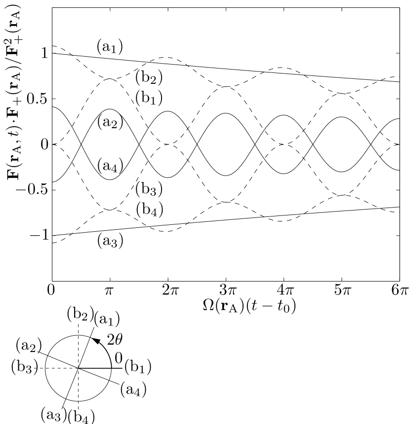
Figure 2: The time dependence of the electric part of the resonant CP force for strong atom–field coupling is displayed for different values of $\theta$, i.e., $2\theta$ $\!=$ $2\theta_{\mathrm{c}}(\mathbf{r}_{\mathrm{A}})$ ($\mathrm{a}_{1}$), $2\theta_{\mathrm{c}}(\mathbf{r}_{\mathrm{A}})\!+\!\pi/2$ ($\mathrm{a}_{2}$), $2\theta_{\mathrm{c}}(\mathbf{r}_{\mathrm{A}})\!+\!\pi$ ($\mathrm{a}_{3}$), $2\theta_{\mathrm{c}}(\mathbf{r}_{\mathrm{A}})\!+\!3\pi/2$ ($\mathrm{a}_{4}$), $\!0$ ($\mathrm{b}_{1}$), $\pi/2$ ($\mathrm{b}_{2}$), $\pi$ ($\mathrm{b}_{3}$), $3\pi/2$ ($\mathrm{b}_{4}$), with parameters $2\theta_{\mathrm{c}}(\mathbf{r}_{\mathrm{A}})$ $\!=$ $3\pi/8$ and $\gamma(\mathbf{r}_{\mathrm{A}})$ $\!=$ $\!0.05\,\Omega(\mathbf{r}_{\mathrm{A}})$. The angles $2\theta$ for the various curves are indicated in the small polar diagram.

where the time dependence of the electric part of the force is displayed for various initial states $|\theta\rangle$ and fixed coupling angle $2\theta_{\mathrm{c}}(\mathbf{r}_{\mathrm{A}})$ $\!=$ $3\pi/8$. The curves in the figure can be grouped in pairs of curves differing only by their sign, each of these pairs corresponds to values of $\theta$ which differ by $2\Delta\theta$ $\!=$ $\!\pi$. The existence of such pairs is an obvious consequence of Eq. (161). The figure further reveals that there are two extremes of behavior: While for the initial states with $2\theta$ $\!=$ $\!2\theta_{\mathrm{c}}(\mathbf{r}_{\mathrm{A}})$, $2\theta_{\mathrm{c}}(\mathbf{r}_{\mathrm{A}})\!+\!\pi$, the force shows no oscillations and is purely exponentially damped as a function of time [curves ($\mathrm{a}_{1}$) and ($\mathrm{a}_{3}$)], the initial states $2\theta$ $\!=$ $2\theta_{\mathrm{c}}(\mathbf{r}_{\mathrm{A}})\!+\!\pi/2$, $2\theta_{\mathrm{c}}(\mathbf{r}_{\mathrm{A}})\!+\!3\pi/2$ lead to oscillations of maximal amplitude around zero [curves ($\mathrm{a}_{2}$) and ($\mathrm{a}_{4}$)]. For other values of $\theta$, the temporal behavior of the force is a superposition of oscillating and non-oscillating components [curves ($\mathrm{b}_{1}$)–($\mathrm{b}_{4}$)].

In the case $2\theta$ $\!=$ $\!0$, which corresponds to the initial state $|1\rangle|\{0\}\rangle$, the oscillating and nonoscillating contributions to the force combine in such a way that the sign of the force remains unchanged for all times [curve ($\mathrm{b}_{1}$)]—in agreement with Eq. (149). The same is valid for the force in the case of the initial state $|0\rangle|1_{\nu}\rangle$ ($2\theta$ $\!=$ $\!\pi$) which has just the opposite global sign [curve ($\mathrm{b}_{3}$)]. At a first glance, one might expect that the respective states evolve into each another during the course of time so that the different global signs would be contradictory. To resolve the apparent contradiction, one must ask whether the initial state $|1\rangle|\{0\}\rangle$ ever evolves into the state $|0\rangle|1_{\nu}\rangle$. A simple calculation reveals that the answer is never: Combining Eqs. (104), (111), (136), (III.2.3), and (III.2.3) for $2\theta$ $\!=$ $\!0$, we find that for the state $|\psi(t)\rangle$ that is initially prepared in the state $|1\rangle|\{0\}\rangle$ the probability $|\psi_{1}(t)|^{2}$ reads

$$|\psi_{1}(t)|^{2}=\cos^{4}[\theta_{c}(\mathbf{r}_{\mathrm{A}})]+\sin^{4}[\theta_{c}(\mathbf{r}_{\mathrm{A}})]+2\cos^{2}[\theta_{c}(\mathbf{r}_{\mathrm{A}})]\\ \times\sin^{2}[\theta_{c}(\mathbf{r}_{\mathrm{A}})]\cos[\Omega(\mathbf{r}_{\mathrm{A}})(t-t_{0})]\\ \geq\cos^{2}[2\theta_{c}(\mathbf{r}_{\mathrm{A}})],$$ (164)

showing that the state $|0\rangle|1_{\nu}\rangle$ is indeed never reached unless in the case of exact resonance, $\Delta(\mathbf{r}_{\mathrm{A}})$ $\!=$ $\!0$ [$\theta_{c}(\mathbf{r}_{\mathrm{A}})$ $\!=$ $\!\pi/4$], where the (resonant parts of the) forces associated with both initial states identically vanish.

Using the same approximations leading from Eq. (143) to Eq. (161), we find that in the limit of strong atom–field coupling, the magnetic component of the force, Eq. (144), can be given as

$$\mathbf{F}_{\theta}^{\mathrm{mag}}(\mathbf{r}_{\mathrm{A}},t)=e^{-\gamma(\mathbf{r}_{\mathrm{A}})(t-t_{0})}\\ \frac{\sin\bigl{\{}2[\theta\!-\!\theta_{\mathrm{c}}(\mathbf{r}_{\mathrm{A}})]\bigr{\}}}{\sin[2\theta_{\mathrm{c}}(\mathbf{r}_{\mathrm{A}})]}\,\cos[\Omega(\mathbf{r}_{\mathrm{A}})(t-t_{0})]\\ \times\mu_{0}\omega_{\nu}\gamma_{\nu}\mathbf{d}_{10}\!\times\!\bigl{[}\mathbf{\nabla}\!\times\!\bm{G}^{(1)}(\mathbf{r},\mathbf{r}_{\mathrm{A}},\omega_{\nu})\!\cdot\!\mathbf{d}_{01}\bigr{]}_{\mathbf{r}=\mathbf{r}_{\mathrm{A}}}.$$ (165)

Comparing this equation with Eq. (161) for the electric component of the force, we see that the magnetic component has a quite different vector structure than the electric one, and its order of magnitude is roughly $\Omega(\mathbf{r}_{\mathrm{A}})/\omega_{\nu}$ times that of the electric component, so that it might become relevant in the context of the recently considered superstrong coupling regime Meiser and Meystre (2006). In particular, the magnetic component of the force vanishes when the system is initially prepared in the state $|\theta\!=\!\theta_{\mathrm{c}}(\mathbf{r}_{\mathrm{A}})\rangle$ or the state $|\theta\!=\!\theta_{\mathrm{c}}(\mathbf{r}_{\mathrm{A}})\!+\!\pi/2\rangle$ for which the electric component of the force is nonoscillating. In all the other cases, the magnetic component is—in contrast to the electric component—always purely oscillating around zero.

Finally, let us compare the nonoscillating force

$$\mathbf{F}_{\pm}(\mathbf{r}_{\mathrm{A}},t)=\mp\frac{\hbar}{2}\,e^{-\gamma(\mathbf{r}_{\mathrm{A}})(t-t_{0})}\bm{\nabla}\!\sqrt{\Omega_{\mathrm{R}}^{2}(\mathbf{r})+\Delta^{2}(\mathbf{r}_{\mathrm{A}})}\big{|}_{\mathbf{r}=\mathbf{r}_{\mathrm{A}}},$$ (166)

which is observed when the system is initially prepared in an approximate energy eigenstate, i.e., $|\theta\!=\!\theta_{\mathrm{c}}(\mathbf{r}_{\mathrm{A}})\rangle$ or $|\theta\!=\!\theta_{\mathrm{c}}(\mathbf{r}_{\mathrm{A}})\!+\!\pi/2\rangle$, with the corresponding static result [Eq. (59) together with Eqs. (50) and (58)]. We see that (i) the static approximation may be regarded as being a good approximation on time scales which are small compared to $\gamma^{-1}(\mathbf{r}_{\mathrm{A}})$, and (ii) the atom–field detuning (110), which enters the force, is different from its bare value (51) due to the coupling with the residual field. However, from Eq. (142) this effect may be expected to be small in general.

IV Summary

Based on macroscopic QED in linear media, we have developed a general theory of the resonant CP force experienced by a two-level atom in the presence of arbitrary linear bodies, with special emphasis on strong atom–field coupling. Assuming that the initial state is a (coherent) superposition of states that carry a single excitation quantum each, we have first worked within a static approximation. Reducing the Hilbert space of the system to an approximately invariant two-dimensional subspace on which the Hamiltonian assumes a Jaynes–Cummings form, the eigenenergies and eigenstates have been constructed according to the well-known dressed-states approach. Identifying the position-dependent part of the eigenenergies with the CP potential for the system being prepared in a dressed state, a simple intuitive picture for the CP force has been obtained, generalizing results obtained for cavities to arbitrary resonator-like equipments.

As the static approximation does not take into account the decay of excited states due to unavoidable radiative and non-radiative losses, the result found for a system prepared in a dressed state is only valid on a time scale which is short compared to the time scale of decay. For systems initially prepared in other than dressed states, the static approximation is even more problematic, because it also neglects the Rabi dynamics which is to be expected in the strong-coupling regime. Motivated by these shortcomings, we have developed an alternative, dynamical approach to the problem by starting from the operator-valued Lorentz force and identifying the CP force with its expectation value where the respective state vector of the system solves the time-dependent Schrödinger equation for given initial condition. By separating the body-assisted field into the part that is in (quasi-)resonance with the atomic transition and strongly interacts with the atom and the residual part that weakly interacts with the atom, we have solved the Schrödinger equation in rotating wave approximation to get a solution which fully incorporates the dynamics induced by both parts of the field. As a consequence, a general expression for the time-dependent resonant CP force has been obtained.

For weak atom–field coupling, this expression reproduces the force obtained earlier for the case where the atom is initially in the upper state and the field is in the vacuum state. The dynamic behavior of the force, which at the initial time effectively agrees with the force obtained in leading-order time-independent perturbation theory, is given by an exponential damping due to spontaneous decay. For strong atom–field coupling, different dynamical behaviors are possible, depending on the initial preparation of the combined system. When the system is prepared in a dressed state, the force which initially agrees with the force obtained in static approximation, undergoes an exponential decay in the further course of time which results from the width of the upper atomic energy level and the width of the body-assisted nonmonochromatic mode. When the initial state is a more general (single excited) state of the atom–field system, then damped Rabi oscillations of the force are observed, whose amplitude and mean value sensitively depend on the chosen initial state. In particular, when the atom is initially excited with the field being in the vacuum state, the force due to the electric field exhibits two major differences with respect to the weak-coupling result: It undergoes damped Rabi oscillations and it is scaled by a correction factor. Furthermore, it has been found that while the dressed-state force is entirely due to the interaction of the atom with the body-assisted electric field, for a more general initial state, additional oscillating force components appear that result from the interaction of the atom with the magnetic field. The general results obtained can be applied to actual geometries by using the appropriate Green tensors, in order to analyze the respective spatial structure of the force in more detail.

Appendix A Single-resonance approximation

Applying Eq. (92), the last term on the r.h.s. of Eq. (103) can be written as

$$-\int_{0}^{\infty}\mathrm{d}\omega\,g^{2}(\mathbf{r}_{\mathrm{A}},\omega)\int_{t_{0}}^{t}\mathrm{d}\tau\,e^{-i(E_{0}/\hbar+\omega)(t-\tau)}\psi_{1}(\tau)\\ =-\int_{0}^{\infty}\mathrm{d}\omega\,g^{\prime 2}(\mathbf{r}_{\mathrm{A}},\omega)\int_{t_{0}}^{t}\mathrm{d}\tau\,e^{-i(E_{0}/\hbar+\omega)(t-\tau)}\psi_{1}(\tau)\\ -\frac{\gamma_{\nu}^{2}}{4}\,g^{2}(\mathbf{r}_{\mathrm{A}},\omega_{\nu})\int_{0}^{\infty}\frac{\mathrm{d}\omega}{(\omega-\omega_{\nu})^{2}+\gamma_{\nu}^{2}/4}\\ \times\int_{t_{0}}^{t}\mathrm{d}\tau\,e^{-i(E_{0}/\hbar+\omega)(t-\tau)}\psi_{1}(\tau),$$ (167)

where, in accordance with the assumptions of the single resonance approximation, the first term may be treated within the Markov approximation. We hence assume that the function $e^{i\tilde{E}_{1}(\mathbf{r}_{\mathrm{A}})t/\hbar}\psi_{1}(t)$ is a slowly varying function, so that

$$- \int_{0}^{\infty}\mathrm{d}\omega\,g^{\prime 2}(\mathbf{r}_{\mathrm{A}},\omega)\int_{t_{0}}^{t}\mathrm{d}\tau\,e^{-i(E_{0}/\hbar+\omega)(t-\tau)}\psi_{1}(\tau)$$

$$\simeq-\psi_{1}(t)\int_{0}^{\infty}\mathrm{d}\omega\,g^{\prime 2}(\mathbf{r}_{\mathrm{A}},\omega)\int_{t_{0}}^{t}\mathrm{d}\tau\,$$

$$\quad\times e^{-i\bigl{[}\hbar\omega-\tilde{E}_{1}(\mathbf{r}_{\mathrm{A}})+E_{0}\bigr{]}(t-\tau)/\hbar}$$

$$\simeq-\psi_{1}(t)\int_{0}^{\infty}\mathrm{d}\omega\,g^{\prime 2}(\mathbf{r}_{\mathrm{A}},\omega)\zeta\bigl{(}\bigl{[}\tilde{E}_{1}(\mathbf{r}_{\mathrm{A}})-E_{0}\bigr{]}/\hbar-\omega\bigr{)}$$ (168)

[$\zeta(x)$ $\!=$ $\!\pi\delta(x)$ $\!+$ $\!i\,\mathcal{P}/x$]. Using Eqs. (25) and (92) as well as the identity

$$\mathcal{P}\int_{0}^{\infty}\frac{\mathrm{d}\omega}{\bigl{[}\tilde{E}_{1}(\mathbf{r}_{\mathrm{A}})-E_{0}\bigr{]}/\hbar-\omega}\,\frac{1}{(\omega-\omega_{\nu})^{2}+\gamma_{\nu}^{2}/4}\\ =\frac{2\pi}{\gamma_{\nu}}\,\frac{\bigl{[}\tilde{E}_{1}(\mathbf{r}_{\mathrm{A}})-E_{0}\bigr{]}/\hbar-\omega_{\nu}}{\bigl{\{}\bigl{[}\tilde{E}_{1}(\mathbf{r}_{\mathrm{A}})-E_{0}\bigr{]}/\hbar-\omega_{\nu}\bigr{\}}^{2}+\gamma_{\nu}^{2}/4}\,,$$ (169)

which can easily be verified by means of contour-integral techniques for $\gamma_{\nu}/2$ $\!\ll$ $\!\omega_{\nu}$, we find

$$-\int_{0}^{\infty}\mathrm{d}\omega\,g^{\prime 2}(\mathbf{r}_{\mathrm{A}},\omega)\int_{t_{0}}^{t}\mathrm{d}\tau\,e^{-i(E_{0}/\hbar+\omega)(t-\tau)}\psi_{1}(\tau)\\ =\Bigl{[}-i\delta\omega^{\prime}_{1}(\mathbf{r}_{\mathrm{A}})-{\textstyle\frac{1}{2}}\Gamma^{\prime}_{1}(\mathbf{r}_{\mathrm{A}})\Bigr{]}\psi_{1}(t),$$ (170)

where we have introduced Eqs. (107)–(110). Substituting this back into Eq. (167) and evaluating the second term by means of Eqs. (44) and (102), we arrive at

$$-\int_{0}^{\infty}\mathrm{d}\omega\,g^{2}(\mathbf{r}_{\mathrm{A}},\omega)\int_{t_{0}}^{t}\mathrm{d}\tau\,e^{-i(E_{0}/\hbar+\omega)(t-\tau)}\psi_{1}(\tau)\\ =\Bigl{[}-i\delta\omega^{\prime}_{1}(\mathbf{r}_{\mathrm{A}})-{\textstyle\frac{1}{2}}\Gamma^{\prime}_{1}(\mathbf{r}_{\mathrm{A}})\Bigr{]}\psi_{1}(t)-{\textstyle\frac{1}{4}}\Omega_{\mathrm{R}}^{2}(\mathbf{r}_{\mathrm{A}})\\ \times\int_{t_{0}}^{t}\mathrm{d}\tau\,e^{[-i(E_{0}/\hbar+\omega_{\nu})-\gamma_{\nu}/2](t-\tau)}\psi_{1}(\tau),$$ (171)

so Eq. (103) can be written in the form

$$\dot{\psi}_{1}(t)=\biggl{[}-i\frac{E_{1}}{\hbar}-i\delta\omega^{\prime}_{1}(\mathbf{r}_{\mathrm{A}})-{\textstyle\frac{1}{2}}\Gamma^{\prime}_{1}(\mathbf{r}_{\mathrm{A}})\biggr{]}\psi_{1}(t)\\ -\textstyle{\frac{1}{2}}i\Omega_{\mathrm{R}}(\mathbf{r}_{\mathrm{A}})\sin\theta\,e^{[-i(E_{0}/\hbar+\omega_{\nu})-\gamma_{\nu}/2](t-t_{0})}\\ -{\textstyle\frac{1}{4}}\Omega_{\mathrm{R}}^{2}(\mathbf{r}_{\mathrm{A}})\int_{t_{0}}^{t}\mathrm{d}\tau\,e^{[-i(E_{0}/\hbar+\omega_{\nu})-\gamma_{\nu}/2](t-\tau)}\psi_{1}(\tau).$$ (172)

By using Eq. (104), this result is transformed to

$$\dot{\phi}_{1}(t)=-\textstyle{\frac{1}{2}}i\Omega_{\mathrm{R}}(\mathbf{r}_{\mathrm{A}})\sin\theta\,e^{\{-i\Delta(\mathbf{r}_{\mathrm{A}})-[\gamma_{\nu}-\Gamma^{\prime}_{1}(\mathbf{r}_{\mathrm{A}})]/2\}(t-t_{0})}\\ -{\textstyle\frac{1}{4}}\Omega_{\mathrm{R}}^{2}(\mathbf{r}_{\mathrm{A}})\int_{t_{0}}^{t}\mathrm{d}\tau\,e^{\{-i\Delta(\mathbf{r}_{\mathrm{A}})-[\gamma_{\nu}-\Gamma^{\prime}_{1}(\mathbf{r}_{\mathrm{A}})]/2\}(t-\tau)}\phi_{1}(\tau)$$ (173)

and after differentiating w.r.t. $t$, we arrive at Eq. (105) together with Eq. (106).

References

• Buhmann and Welsch (2007) S. Y. Buhmann and D.-G. Welsch, Prog. Quantum Electron. 31, 51 (2007).
• Casimir and Polder (1948) H. B. G. Casimir and D. Polder, Phys. Rev. 73, 360 (1948).
• Wylie and Sipe (1985) J. M. Wylie and J. E. Sipe, Phys. Rev. A 32, 2030 (1985).
• Jaynes and Cummings (1963) E. T. Jaynes and F. W. Cummings, Proc. IEEE 51, 89 (1963).
• Haroche et al. (1991) S. Haroche, M. Brune, and J. M. Raimond, Europhys. Lett. 14, 19 (1991).
• Englert et al. (1991) B.-G. Englert, J. Schwinger, A. O. Barut, and M. O. Scully, Europhys. Lett. 14, 25 (1991).
• Prants and Sirotkin (2001) S. V. Prants and V. Y. Sirotkin, Phys. Rev. A 64, 033412 (2001).
• Battocletti and Englert (1994) M. Battocletti and B.-G. Englert, J. Phys. II 4, 1939 (1994).
• Bastin and Martin (2003) T. Bastin and J. Martin, Phys. Rev. A 67, 053804 (2003).
• Retamal et al. (1998) J. C. Retamal, E. Solano, and N. Zagury, Opt. Commun. 154, 28 (1998).
• Löffler et al. (1998) M. Löffler, G. M. Meyer, and H. Walther, Europhys. Lett. 41, 593 (1998).
• Bastin and Martin (2004) T. Bastin and J. Martin, Eur. Phys. J. D 29, 133 (2004).
• An et al. (2000) K. An, Y.-T. Chough, and S.-H. Youn, Phys. Rev. A 62, 023819 (2000).
• Buhmann et al. (2004) S. Y. Buhmann, L. Knöll, D.-G. Welsch, and D. T. Ho, Phys. Rev. A 70, 052117 (2004).
• Buhmann et al. (2005) S. Y. Buhmann, D. T. Ho, T. Kampf, and D.-G. Welsch, Eur. Phys. J. D 35, 15 (2005).
• Ren and Carmichael (1995) W. Ren and H. J. Carmichael, Phys. Rev. A 51, 752 (1995).
• Doherty et al. (1997) A. C. Doherty, A. S. Parkins, S. M. Tan, and D. F. Walls, Phys. Rev. A 56, 833 (1997).
• Doherty et al. (2000) A. C. Doherty, T. W. Lynn, C. J. Hood, and H. J. Kimble, Phys. Rev. A 63, 013401 (2000).
• Pinkse et al. (2000a) P. H. W. Pinkse, T. Fischer, P. Maunz, and G. Rempe, Nature 404, 365 (2000a).
• Hood et al. (2000) C. J. Hood, T. W. Lynn, A. C. Doherty, A. S. Parkins, and H. J. Kimble, Science 287, 1447 (2000).
• Pinkse et al. (2000b) P. W. H. Pinkse, T. Fischer, P. Maunz, T. Puppe, and G. Rempe, J. Mod. Opt. 47, 2769 (2000b).
• Hood et al. (2001) C. J. Hood, T. W. Lynn, A. C. Doherty, D. W. Vernooy, J. Ye, and H. J. Kimble, Laser Phys. 11, 1190 (2001).
• Mabuchi et al. (1996) H. Mabuchi, Q. A. Turchette, M. S. Chapman, and H. J. Kimble, Opt. Lett. 21, 1393 (1996).
• Münstermann et al. (1999a) P. Münstermann, T. Fischer, P. W. H. Pinkse, and G. Rempe, Opt. Commun. 159, 63 (1999a).
• Münstermann et al. (1999b) P. Münstermann, T. Fischer, P. Maunz, P. W. H. Pinkse, and G. Rempe, Phys. Rev. Lett. 82, 3791 (1999b).
• Fischer et al. (2002) T. Fischer, P. Maunz, P. W. H. Pinkse, T. Puppe, and G. Rempe, Phys. Rev. Lett. 88, 163002 (2002).
• Ho et al. (2003) D. T. Ho, S. Y. Buhmann, L. Knöll, D.-G. Welsch, S. Scheel, and J. Kästel, Phys. Rev. A 68, 043816 (2003).
• Raabe and Welsch (2007) C. Raabe, S. Scheel, and D.-G. Welsch, Phys. Rev. A 75, 053813 (2007).
• Meiser and Meystre (2006) D. Meiser and P. Meystre, Phys. Rev. A 74, 065801 (2006).