Scattering quantum random-walk search with errors

Abstract

We analyze the realization of a quantum-walk search algorithm in a passive, linear optical network. The specific model enables us to consider the effect of realistic sources of noise and losses on the search efficiency. Photon loss uniform in all directions is shown to lead to the rescaling of search time. Deviation from directional uniformity leads to the enhancement of the search efficiency compared to uniform loss with the same average. In certain cases even increasing loss in some of the directions can improve search efficiency. We show that while we approach the classical limit of the general search algorithm by introducing random phase fluctuations, its utility for searching is lost. Using numerical methods, we found that for static phase errors the averaged search efficiency displays a damped oscillatory behaviour that asymptotically tends to a non-zero value.

I Introduction

The generalization of random walks for quantum systems Aharonov et al. (1993) proved to be a fruitful concept Kempe (2003) attracting much recent interest. Algorithmic application for quantum information processing is an especially promising area of utilization of quantum random walks (QRW) Ambainis (2004).

In his pioneering paper Grover (1996) Grover presented a quantum algorithm that can be used to search an unsorted database quadratically faster than the existing classical algorithms. Shenvi, Kempe and Whaley (SKW) Shenvi et al. (2003) proposed a search algorithm based on quantum random walk on a hypercube, which has similar scaling properties as the Grover search. In the SKW algorithm the oracle is used to modify the quantum coin at the marked vertex. In contrast to the Grover search, this algorithm generally has to be repeated several times to produce a result, but this merely adds a fixed overhead independent of the size of the search space.

There are various suggestions and some experiments how to realize quantum walks in a laboratory. The schemes proposed specifically for the implementation of QRWs include ion traps Travaglione and Milburn (2002), nuclear magnetic resonance Du et al. (2003) (also experimentally verified Ryan et al. (2005)), cavity quantum electrodynamics Di et al. (2004); Agarwal and Pathak (2005), optical lattices Dur et al. (2002), optical traps Eckert et al. (2005), optical cavity Roldan and Soriano (2005), and classical optics Knight et al. (2003). Moreover, the application of standard general logic networks to the task is always at hand Hines and Stamp (2007); Fujiwara et al. (2005).

The idea of the scattering quantum random walk (SQRW) Hillery et al. (2003) was proposed as an answer to the question that can be posed as: how to realize a coined walk by a quantum optical network built from passive, linear optical elements such as beam splitters and phase shifters? It turned out that such a realization is possible and, in fact, it leads to a natural generalization of the coined walk, the scattering quantum random walk Košik and Bužek (2005). The SQRW on the hypercube allows for a quantum optical implementation of the SKW search algorithm Shenvi et al. (2003). Having a proposal for a physical realization at hand we are in the position to analyze in some detail the effects hindering its successful operation.

Noise and decoherence strongly influence quantum walks. For a recent review on this topic see Kendon (2006). The first investigations in this direction indicated that a small amount of decoherence can actually enhance the mixing property Kendon and Tregenna (2003). For a continuous QRW on a hypercube there is a threshold for decoherence, beyond which the walk behaves classically Alagic and Russell (2005). Košik et al analyzed SQRW with randomized phase noise on a $d$ dimensional lattice Košik et al. (2006). The quantum walk on the line has been studied by several authors in the linear optical context, with the emphasis on the effect of various initial states, as well as on the impact of decoherence Jeong et al. (2004); Pathak and Agarwal (2007). The quantum random walk search with imperfect gates was discussed in some detail by Li et al Li et al. (2006), who have considered the case when the Grover operator applied in the search is systematically modified. Such an imperfection decreases the search probability and also shifts its first maximum in time.

In this paper we analyze the impact of noise on the SKW algorithm typical for the experimental situations of the SQRW. In particular, first we focus on photon losses and show that, somewhat contradicting the naïve expectation, non-trivial effects such as the enhancement of the search efficiency can be observed. As a second type of errors we study randomly distributed phase errors in two complementary regimes. The first regime is characterized by rapid fluctuation of the optical path lengths, that leads to the randomization of phases for each run of the algorithm. We show that the classical limit of the SKW algorithm, reached by increasing the variance of the phase fluctuations, does not correspond to a search algorithm. In the other regime, the stability of the optical path lengths is maintained over the duration of one run, thus the errors are caused by static random phases. This latter case has not yet been considered in the context of QRWs. We found that static phase errors bring a significantly different behaviour compared to the case of phase fluctuations. Under static phase errors the algorithm retains its utility, with the average success probability displaying a damped oscillatory behaviour that asymptotically tends to a non-zero constant value.

The paper is organized as follows. In the next section we introduce the scattering quantum walk search algorithm. In section III. we derive analytic results for the success probability of search for the case when a single coefficient describes photon losses independent of the direction. In section IV. we turn to direction dependent losses, and present estimations of the success probability based on analytical calculations and numerical evidence. In section V. phase noise is considered and consequences for the success probability are worked out. Finally, we conclude in Sec. VI.

II The scattering quantum walk search algorithm

The quantum walk search algorithm is based on the generalized notion of coined quantum random walk (CQRW), allowing the coin operator to be non-uniform accross the vertices. In the early literature the coin is considered as position (vertex) independent. The CQRW is defined on the product Hilbert space ${\mathcal{H}}={\mathcal{H}}^{C}\otimes{\mathcal{H}}^{G}$, where ${\mathcal{H}}^{C}$ refers to the quantum coin, and ${\mathcal{H}}^{G}$ represents the graph on which the walker moves. The discrete time-evolution of the system is governed by the unitary operator

$$U=SC\,,$$ (1)

where $C$ is the coin operator which corresponds to flipping the quantum coin, and $S$ is the step or translation operator that moves the walker one step along some outgoing edge, depending on the coin state. Adopting a binary string representation of the vertices $V$ of the underlying graph $G=(V,E)$, the step operator $S$ (a permutation operator of the entire Hilbert space ${\mathcal{H}}$) can be expressed as

$$S=\sum_{d=0}^{n-1}\sum_{x\in V}\left|d,x\oplus e_{dx}\right>\left<d,x\right|\,.$$ (2)

In (2) $x$ denotes the vertex index. Here, and in the rest of this paper we identify the vertices with their indices and understand $V$ as the set of vertex indices. The most remarkable fact about $S$ is that it contains all information about the topology of the graph. In particular, the actual binary string values of $e_{dx}$ are determined by the set of edges $E$. This is accomplished by the introduction of direction indices $d$, which run from $0$ to $n-1$ in case of the $n$ regular graphs which are used in the search algorithm.

To implement the scattering quantum random walk on an $n$ regular graph of $N$ nodes, identical $n$-multiports Jex et al. (1995); Żukowski et al. (1997) are arranged in columns each containing $N$ multiports. The columns are enumerated from left to right, and each row is assigned a number sequentially. The initial state enters on the input ports of multiports in the leftmost column. The output and input ports of multiports of neighbouring columns $j$ and $j+$ are then indexed suitably and connected according to the graph $G$.

For the formal description of quantum walks on arrays of multiports, we propose to label every mode by the row index and input port index of its destination multiport. We note that an equally good labelling can be defined using the row index and output port index of the source multiport. To describe single excitation states, we use the notation $\left|d,x\right>$ where the input port index of the destination multiport is $d=0,1,\ldots,n-1$, and the row index is $x=0,1,\ldots,N-1$. Thus the total Hilbert space can effectively be separated into some product space ${\mathcal{H}}^{C}\otimes{\mathcal{H}}^{G}$. To be precise, the additional label $j$ would be necessary to identify in which column the multiport is, however, we think of the column index as a discrete time index, and drop it as an explicit label of modes. Thus a time-evolution $U=SC$ can be generated by the propagation through columns of multiports.

A quantum walk can be realized in terms of the basis defined using the destination indices, and we shall term it “standard basis” through this section. First, we recall that an $n$-multiport can be fully characterized by an SU($n$) transformation matrix $\mathbf{C}$. The effect of such multiport on single excitation states $\left|\psi\right>\in{\mathcal{H}}^{C}$ is given by the formula,

$$\left|\psi\right>=\sum_{d=0}^{n-1}a_{d}\left|d\right>\to\sum_{d,k=0}^{n-1}C_{dk}a_{k}\left|d\right>,$$ (3)

where $\left|d\right>$ denotes the single photon state with the photon being in the $d$ mode, i.e. $\left|d\right>=\left|0\right>_{0}\ldots\left|1\right>_{d}\ldots\left|0\right>_{n-1}$. We note, that a multiport with any particular transformation matrix $\mathbf{C}$ can be realized in a laboratory Reck et al. (1994). To simplify calculations it may be beneficial to choose an indexing of input and output ports such that the connections required to realize the graph $G$ can be made in such way that each input port has the same index as the corresponding source output port. Therefore the label $d$ can stay unique during “propagation.” We emphasize that this is not a necessary assumption for a proper definition of SQRW, but an important property that makes also easier to see that SQRWs are a superset of generalized CQRWs. This indexing of input and output ports for walks on a hypercube is depicted on Fig. 1a, with some of the actual connections illustrated for a (three dimensional) cube on Fig. 1b.

Considering an array of identical multiports, an arbitrary input state undergoes the transformation by the same matrix $\mathbf{C}$ for every $x$. Let the output port $d$ of multiport $x$ be connected to multiport $x\oplus e_{dx}$ in the next row. Thus the mode labelled by the source indices $d$ and $x$, is labelled by $d$ and $x\oplus e_{dx}$ in terms of the destination indices. Therefore, effect of propagation in terms of our standard basis is written,

$$\sum_{d,x}a_{dx}\left|d,x\right>\to\sum_{dkx}C_{dk}a_{kx}\left|d,x\oplus e_{dx}\right>.$$ (4)

Comparing this formula with Eqs. (2) and (3) we see that this formula corresponds to a $U=SC=S(C_{0}\otimes\openone)$ transformation where $C_{0}$ is generated by the matrix $\mathbf{C}$. Due to the local nature of the realization of the coin operation, it is straight-forward to realize position dependent coin operations, such as the one required for the quantum walk search algorithm.

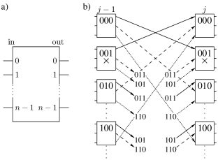
Figure 1: a) Illustration of the labelling of input and output ports of multiports used for the realization of the walk on the $n$ dimensional hypercube. b) Schematic depiction of the setup of the SQRW implementation of the SKW algorithm for $n=3$, with the marked node being $x_{\mathrm{t}}=001$. For clarity, a unique line pattern is associated with each input (output) port index.

In particular, the SKW algorithm Shenvi et al. (2003) is based on the application of two distinct coin operators, e.g.

$$C_{0} = G,$$ (5a)

$$C_{1} = -\openone,$$ (5b)

where $G$ is the Grover inversion or diffusion operator $G:=-\openone+2|s^{C}\rangle\langle s^{C}|$, with $|s^{C}\rangle=1/\sqrt{n}\sum_{d=1}^{n}\left|d\right>$ Moore and Russell (2002). In the algorithm, the application of the two coin operators is conditioned on the result of oracle operator ${\mathcal{O}}$. The oracle marks one $x_{\mathrm{t}}$ as target, hence the coin operator becomes conditioned on the node:

$$C^{\prime}=C_{0}\otimes\openone+(C_{1}-C_{0})\otimes\left|x_{\mathrm{t}}\right>\left<x_{\mathrm{t}}\right|.$$ (6)

When $n$ is large, the operator $U^{\prime}:=SC^{\prime}$ can be regarded as a perturbed variation of $U=S(C_{0}\otimes\openone)$. The conditional transformation (6) is straight-forward to implement in the multiport network. For the two coins (5) one has to use a simple phase shifter at position $x_{\mathrm{t}}$ in every column of the array, and a multiport realizing the Grover matrix $G$ at every other position. The connection topology required to implement a walk on the hypercube is such that in the binary representation we have $e_{d}=0\ldots 1\ldots 0$ with 1 being at the $d$’th position, i.e. $e_{d}=2^{d}$. See Fig. 1b for a schematic example, when $x_{\mathrm{t}}=001$.

The above described scheme to realize quantum walks in an array of multiports using as many columns as the number of iterations of $U$ can be reduced to only a single column. To do this, one simply needs to connect the output ports back to the appropriate input ports of the destination multiport in the same column. This feed-back setup is similar to the one introduced in Ref. Košik and Bužek (2005).

III Uniform decay

We begin our analysis of the effect of errors on the quantum walk search algorithm by concentrating on photon losses. In an optical network, photon losses are usually present due to imperfect optical elements. An efficient model for linear loss is to introduce fictitious beam-splitters with transmittances corresponding to the effective transmission rate (see Fig. 2).

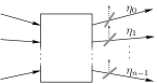
Figure 2: Schematic illustration of the photon loss model being used. The losses suffered by each output mode are represented by fictitious beam-splitters with transmittivities $\eta_{d}$. The beam-splitters incorporate the combined effect of imperfections of the multiport devices, and effects influencing the state during propagation between the multiports (e.g. scattering and absorption).

The simplest case is when all arms of the multiports are characterized by the same linear loss rate $\eta$. The operator describing the effect of decay on a single excitation density operator can then be expressed as

$${\mathcal{D}}(\varrho)=\eta^{2}\varrho+(1-\eta^{2})\left|0\right>\!\left<0\right|.$$ (7)

The total evolution of the system after one iteration may be written as $\varrho\to{\mathcal{D}}(U\varrho U^{{\dagger}})$. It is important to note that with the introduction of this error, the original Hilbert space ${\mathcal{H}}^{G}$ of one-photon excitations must be extended by the addition of the vacuum state $\left|0\right>$. The action of the SQRW evolution operator $U$ on the extended Hilbert space follows from the property $U\left|0\right>=\left|0\right>$. Due to the nature of Eq. (7) and the extension of $U$, one can see that the order of applying the unitary time step and the error operator ${\mathcal{D}}$ can be interchanged. Therefore, over $t$ steps the state of the system undergoes the transformation

$$\varrho\to\eta^{2t}U^{t}\varrho U^{{\dagger}t}+(1-\eta^{2t})\left|0\right>\!\left<0\right|={\mathcal{D}}^{t}(U^{t}\varrho U^{{\dagger}t}).$$ (8)

To simplify calculations, we introduce a linear (but non-unitary) operator to denote the effect of the noise operator ${\mathcal{D}}$ on the search Hilbert space:

$$D\left|\psi\right>=\eta\left|\psi\right>.$$ (9)

This operator is simply a multiplication with a number. It is obviously linear, however, for $\eta<1$ not unitary. The operator $D$ does not describe any coherence damping within the one-photon subspace, since it only uniformly decreases the amplitude of the computational states and introduces the vacuum. Since all final statistics are gathered from the search Hilbert space ${\mathcal{H}}^{G}$, it is possible to drop the vacuum from all calculations, and incorporate all information related to it into the norm of the remaining state. In other words, we can think of $DU$ as the time step operator, and relax the requirement of normalization. Using this notation, the effect of $t$ steps is very straight-forward to express:

$$\left|\psi\right>\to\eta^{t}U^{t}\left|\psi\right>.$$ (10)

This formula indicates that inclusion of the effect of uniform loss may be postponed until just before the final measurement. The losses, therefore, may simply be included in the detector efficiency (using an exponential function of the number of iterations).

Applying the above model of decay to the quantum walk search algorithm we define the new step operator $U^{\prime\prime}=DU^{\prime}$, and write the final state of the system after $t$ steps as

$$(U^{\prime\prime})^{t}\left|\psi_{0}\right>=\\ \eta^{t}\cos(\omega^{\prime}_{0}t)\left|\psi_{0}\right>-\eta^{t}\sin(\omega^{\prime}_{0}t)\left|\psi_{1}\right>+\eta^{t}O\left(\frac{n^{3/4}}{\sqrt{2^{n}}}\right)\left|\tilde{r}\right>.$$ (11)

Adopting the notation of Ref. Shenvi et al. (2003), the probability of measuring the target state $\left|x=0\right>$ at the output after $t$ steps can be expressed as

$$p_{n}(\eta,t)=\sum_{d=0}^{n-1}\left|\left<d,0\left|(U^{\prime\prime})^{t}\psi_{0}\right.\right>\right|^{2}\\ =\eta^{2t}\sin^{2}(\omega^{\prime}_{0}t)\left|\left<\left.R,0\right|\psi_{1}\right>\right|^{2}+2^{-n}\eta^{2t}\cos^{2}(\omega^{\prime}_{0}t)\\ +O(1/2^{n}).$$ (12)

We know from Ref. Shenvi et al. (2003) that $\left|\left<\left.R,0\right|\psi_{1}\right>\right|^{2}=1/2-O(1/n)$. Since an overall exponential drop of the success probability is expected due to the $\eta^{2t}$ factor, we search for the maximum $t_{f}$ be before the ideal time-point $|\omega^{\prime}_{0}|t=\pi/2$. This guarantees that $\sin^{2}(\omega^{\prime}_{0}t_{f})$ is finite, therefore due to the $2^{-n}$ factor for large $n$ the second term can be omitted, and it is sufficient to maximize the function

$$p_{n}(\eta,t)=\eta^{2t}\sin^{2}(\omega^{\prime}_{0}t)\left(1/2-O(1/n)\right),$$ (13)

with respect to $t$. After substituting the result $|\omega^{\prime}_{0}|=1/\sqrt{2^{n-1}}[1-O(1/n)]\pm O(n^{3/2}/2^{n})$ from Ref. Shenvi et al. (2003), these considerations yield the global maximum at $t_{f}=\sqrt{2^{n-1}}\left[\mathop{\mathrm{acot}}\nolimits(-\ln\eta\sqrt{2^{n-1}})+O(1/n)\right]$. During operation we set

$$t_{m}:=\sqrt{2^{n-1}}\mathop{\mathrm{acot}}\nolimits(-\ln\eta\sqrt{2^{n-1}}),$$ (14)

or the closest integer, as the time yielding the maximum probability of success.

To simplify the upcoming formulae, we introduce the variables

$$x = -\ln\eta\ \sqrt{2^{n-1}},$$ (15)

$$\varepsilon = \log_{2}(1-\eta).$$ (16)

The variable $\varepsilon$ can be regarded as a logarithmic transmission parameter (the ideal case corresponds to $\varepsilon=\infty$, and complete loss to $\varepsilon=0$). When $\varepsilon$ is sufficiently large, the expression $-\ln\eta$ can be approximated to first order in $2^{-\varepsilon}$ and we obtain

$$x\approx 2^{-\varepsilon+n/2-1/2}.$$ (17)

Upon substituting $t_{m}$ into (13) we can use the new variable $x$ to express the sine term as

$$\sin^{2}(\omega^{\prime}_{0}t_{m})=\sin^{2}(|\omega^{\prime}_{0}|t_{m})=\sin^{2}\left[\mathop{\mathrm{acot}}\nolimits x(1+O(1/n))\right]=\\ =\frac{1}{1+x^{2}}+\frac{2x\mathop{\mathrm{acot}}\nolimits x}{1+x^{2}}O(1/n)+\frac{\mathop{\mathrm{acot}}\nolimits^{2}x}{1+x^{2}}O(1/n^{2}).$$ (18)

Thus for the maximum success probability $p_{n}^{\mathrm{max}}(\eta)=p_{n}(\eta,t_{m})$ we obtain

$$p_{n}^{\mathrm{max}}(\eta)=\frac{e^{-2x\mathop{\mathrm{acot}}\nolimits x}}{1+x^{2}}\left[\frac{1}{2}-O(1/n)+x\mathop{\mathrm{acot}}\nolimits x\,O(1/n)\right].$$ (19)

This formula is our main result for the case of uniform photon losses. In the large $n$ limit it gives the approximate performance of the SKW search algorithm as a function of the transmission rate and the size of the search space. Since $x\mathop{\mathrm{acot}}\nolimits x$ is bounded in $x$, the accuracy of the term in brackets is bounded by $O(1/n)$. The most notable consequence of the second $O(1/n)$ contribution is that while in the ideal case the probability $1/2$ is an upper bound, in the lossy case deviations from the leading term,

$$p^{\mathrm{max}}(x)=\frac{1}{2}\exp(-2x\mathop{\mathrm{acot}}\nolimits x)\frac{1}{1+x^{2}},$$ (20)

can be expected in either direction. The functional form of Eq. (20), plotted on Fig. 3, allows for a universal interpretation of the dependence of success probability on the transmission rate and the size of the search space through the combined variable $x$. For small losses we can use the approximation (17) and conclude that the search efficiency depends only on the difference $n/2-\varepsilon$. The approximation is compared with the results of numerical calculations on Fig. 4. We can observe the $O(1/n)$ accuracy of the theoretical curves as expected, hence producing poorer fits at smaller ranks. The positive deviations from the theoretical curves observable at low transmission rates are due to the second $O(1/n)$ term of Eq. (19).

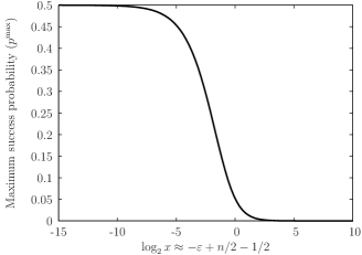
Figure 3: Probability of measuring the target state after the optimal number of iterations according to the approximation in Eq. (20). The probability is plotted against the logarithm of $x$ which is a combination of the rank of the hypercube $n$ and the logarithmic transmission parameter $\varepsilon$.

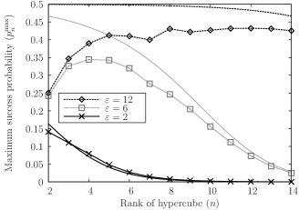
Figure 4: Maximum success probabilities for different ranks of hypercube ($n$) calculated using the theoretical approximation, and numerical simulations. The theoretical curves are drawn with continuous lines of different patterns, and the numerical results are represented by points interconnected with the same line pattern and colour as the theoretical approximates corresponding to the same logarithmic transmission parameter $\varepsilon$.

IV Direction dependent loss

In the present section we no longer assume equal loss rates, and consider the schematically depicted loss model on Fig. 2 with arbitrary $\eta_{d}$ parameters. Because of the high symmetry of the hypercube graph, and the use of mainly identical multiports, we can neglect the position dependence of the transmission coefficients. The operator ${\mathcal{D}}$ describing the decoherence mechanism thus acts on a general term of the density operator as

$${\mathcal{D}}(\left|d,x\right>\left<d^{\prime},x^{\prime}\right|)=\eta_{d}\eta_{d^{\prime}}\left|d,x\right>\left<d^{\prime},x^{\prime}\right|+\delta_{xx^{\prime}}\delta_{dd^{\prime}}\eta_{d}^{2}\left|0\right>\!\left<0\right|.$$ (21)

To describe the overall effect of this operator on a pure state, we re-introduce the linear decoherence operator in a more general form,

$$D=\sum_{d}\eta_{d}\left|d\right>\left<d\right|\otimes\openone,$$ (22)

and use the notation $\{\eta\}$ to denote the set of coefficients $\eta_{d}$. Due to the symmetry of the system, the sequential order of coefficients is irrelevant. With the re-defined operator the effect of decoherence reads

$${\mathcal{D}}(\varrho)=\varrho^{\prime}+(1-\mathop{\mathrm{Tr}}\nolimits\varrho^{\prime})\left|0\right>\!\left<0\right|,$$ (23)

where $\varrho=\left|\psi\right>\left<\psi\right|$ is the initial state, and the non-vacuum part of the output state is $\varrho^{\prime}=\left|\psi^{\prime}\right>\left<\psi^{\prime}\right|$, with $\left|\psi^{\prime}\right>=D\left|\psi\right>$. Therefore, we can again reduce our problem to calculating the evolution of unnormalized pure states, just as in the uniform case, and use the non-unitary step operator $U^{\prime\prime}=DU^{\prime}$ with the more general noise operator.

Telling how well the algorithm performs under these conditions is a complex task. First we give a lower bound on the probability of measuring the target node, based on generic assumptions. To begin, we separate the noise operator into two parts

$$D=\eta+D^{\prime},$$ (24)

where, for the moment, we leave $0\leq\eta\leq 1$ undefined. As a consequence of Eq. (22) the diagonal elements of $D^{\prime}$ are $[D^{\prime}]_{dd}=\delta_{d}=\eta_{d}-\eta$, and the off-diagonal elements are zero. From Eq. (23) it follows that starting from a pure state $\left|\psi_{0}\right>$, after $t$ non-ideal steps the state of the system can be characterized by the unnormalized vector $\left|\psi^{\prime}(t)\right>$, which is related to the state obtained from the same initial state by $t$ ideal steps as

$$\left|\psi^{\prime}(t)\right>=\eta^{t}\left|\psi(t)\right>+\left|r\right>.$$ (25)

The expression of the residual vector $\left|r\right>$ reads

$$\left|r\right>=\sum_{k=1}^{t}(DU^{\prime})^{t-k}D^{\prime}\eta^{k-1}\left|\psi(k)\right>.$$ (26)

To obtain the probability of measuring the target state $\left|x=0\right>$ we have to evaluate the formula

$$p_{n}(\{\eta\},t)=\sum_{d=0}^{n-1}\left|\eta^{t}\left<\left.d,0\vphantom{\psi(t)}\right|\psi(t)\right>+\left<\left.d,0\vphantom{r}\right|r\right>\right|^{2}.$$ (27)

Due to the symmetry of the graph and the coins, we use e.g. Eq. (13) and obtain $\left<\left.d,0\vphantom{\psi(t)}\right|\psi(t)\right>\approx-\sin(\omega^{\prime}_{0}t)/\sqrt{2n}$. To obtain a lower bound on $p_{n}(\{\eta\},t)$ we note that the sum is minimal if $\left<\left.d,0\vphantom{r}\right|r\right>=\textrm{const}=K$ for every $d$ (we consider a worst case scenario when all $\left<\left.d,0\vphantom{r}\right|r\right>$ are negative). Now we assume that the second term is a correction with an absolute value smaller than that of the first term. For the upper bound on $K$, we use the inequality

$$\sum_{d=0}^{n-1}\left|\left<\left.d,0\vphantom{r}\right|r\right>\right|^{2}\leq\left<\left.r\vphantom{r}\right|r\right>.$$ (28)

The norm of $\left|r\right>$ can be bound using the eigenvalues of $U$, $D$, and $D^{\prime}$. Let $\eta_{\mathrm{max}}=\max\left\{\eta_{d}|d=0,\ldots,n-1\right\}$ and $\delta_{\mathrm{max}}=\max\left\{\left|\delta_{d}\right||d=0,\ldots,n-1\right\}$. Then we have

$$\left<\left.r\vphantom{r}\right|r\right>\leq\sum_{k=1}^{t}\eta_{\mathrm{max}}^{t-k}\delta_{\mathrm{max}}\eta^{k-1}=\frac{\eta_{\mathrm{max}}}{\eta}\frac{\delta_{\mathrm{max}}}{\eta_{\mathrm{max}}-\eta}(\eta_{\mathrm{max}}^{t}-\eta^{t}).$$ (29)

Since $U$ is unitary, its contribution to the above formula is trivial. Our upper bound on $|K|$ hence becomes $|K|\leq 1/{\sqrt{n}}(\eta_{\mathrm{max}}\delta_{\mathrm{max}}/\eta)(\eta_{\mathrm{max}}^{t}-\eta^{t})/(\eta_{\mathrm{max}}-\eta)$. Combining the results, we obtain a lower bound on the probability for measuring the target node,

$$p_{n}(\{\eta\},t)\geq\eta^{2t}\left\{\sqrt{p_{n}^{(i)}(t)}\right.\\ \left.-\frac{\eta_{\mathrm{max}}}{\eta}\frac{\delta_{\mathrm{max}}}{\eta_{\mathrm{max}}-\eta}\left[\left(\frac{\eta_{\mathrm{max}}}{\eta}\right)^{t}-1\right]\right\}^{2},$$ (30)

where $p_{n}^{(i)}(t)$ stands for the corresponding probability of the ideal (lossless) case. We maximize the lower bound with respect to the arbitrary parameter $\eta$. The procedure can be carried out noting that $\delta_{\mathrm{max}}=\max\{\eta_{\mathrm{max}}-\eta,\eta-\eta_{\mathrm{min}}\}$, thereby we find the maximum at $\eta=\bar{\eta}\equiv(\eta_{\mathrm{max}}+\eta_{\mathrm{min}})/2$, yielding the formula

$$p_{n}(\{\eta\},t)\geq\bar{\eta}^{2t}\left\{\sqrt{p_{n}^{(i)}(t)}-({\eta_{\mathrm{max}}}/{\bar{\eta}})\left[\left({\eta_{\mathrm{max}}}/{\bar{\eta}}\right)^{t}-1\right]\right\}^{2}.$$ (31)

To interpret the formula (31), we consider the two terms in the curly braces separately. The first term returns the success probability for uniform losses with transmission coefficient $\bar{\eta}$. The second term may be considered as a correction term that depends not only on some average value of the loss distribution, but also on its degree of non-uniformity in a way that is reminiscent of a mean square deviation. We observe that Eq. (30) provides a useful lower bound only for $\{\eta\}$ distributions violating uniformity to only a small degree. When the expression inside the curly braces becomes negative, the assumption made on the magnitude of the second term of Eq. (27) becomes invalid, and therefore the formula does not give a correct lower bound.

The estimated lower bound (30) decreases with increasing degree of non-uniformity, in accordance with a naive expectation. However, as we shall show later, numerical simulations taking into account the full complexity of the problem provide evidence to the contrary: departure from uniformity can result in improved efficiency.

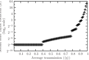
Figure 5: The coefficients for the $\left<\eta\right>$ dependent second order term in the Taylor series expansion of $p_{n}^{\mathrm{\max}}(\{\eta\})$. The coefficients have been obtained by second order fitting to numerically generated values for a hypercube sized $n=8$. The confidence of each fit is represented on the graph by an error bar. It is clearly visible that the coefficients are always greater than $2^{-n}$. Another feature, that is more suggestive on a linear scale, is that the points between two steps seem to align into straight lines, with their slopes increasing with $\left<\eta\right>$.

Inspired by the appearance of the average loss rate in the lower bound (31), we introduce the mean and the variance of the direction dependent losses,

$$\left<\eta\right>=\frac{1}{n}\sum_{d=0}^{n-1}\eta_{d},\quad\mbox{and}\quad Q=\frac{1}{n}\sum_{d=0}^{n-1}\delta_{d}^{2}.$$ (32)

By using the Taylor expansion of the success probability function $p_{n}^{\mathrm{max}}$ around the point $\eta_{d}=\left<\eta\right>$, the deviations from the uniform loss case can be well estimated at small degrees of non uniformity. Using the permutation symmetry of $p_{n}^{\mathrm{max}}$ we can express the Taylor series as

$$p_{n}^{\mathrm{max}}(\{\eta\})=p_{n}^{\mathrm{max}}(\left<\eta\right>)+BQ^{2}+CW^{3}+O(\delta_{d}^{4}),$$ (33)

where $W^{3}=1/n\sum_{k}\delta_{k}^{3}$. We notice that $Q$ may be regarded as the mean deviation of $\{\eta\}$ as a distribution, and hence it is a well-defined statistical property of the random noise. In other words, as long as a second order Taylor expansion gives an acceptable approximation, the probability of success depends only on the statistical average and variance ($\left<\eta\right>$, $Q$) of the noise and not on the specific values of $\{\eta\}$. Using numerical simulations, we have determined the values of $B$ up to rank $n=10$, and studied the impact of higher order terms.

The second order Taylor coefficients were determined by fitting over the numerically obtained success probabilities at data points where the higher order moments of the loss distributions were small. An example plot of $B$ is provided on Fig. 5, for a system $n=8$. The higher order effects were suppressed by selecting the lowest values of $W$ from several repeatedly generated random distributions $\{\eta\}$. A general feature exhibited by all studied cases is that the second order coefficients satisfy the inequality

$$B\geq 2^{-n}.$$ (34)

It is remarkable that this tight lower bound depends only on the size of the system. The dependence of $B$ on $\left<\eta\right>$ is monotonous with discontinuities. We found the number of discontinuities to be proportional to the rank $n$. Our numerical studies have shown that the value of $B$ before the first discontinuity is always a constant, and equal to the empirical lower bound (34).

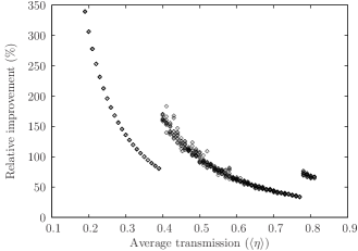
Figure 6: The relative improvement of maximum success probability comparing direction dependent loss to uniform loss with identical average loss rates. The difference is measured as $[p_{n}^{\mathrm{max}}(\{\eta\})-p_{n}^{\mathrm{max}}(\left<\eta\right>)]/p_{n}^{\mathrm{max}}(\left<\eta\right>)$. All points were generated at $Q=0.35$ and the entire available domain for $\left<\eta\right>$. The values of higher moments of $\{\eta\}$ are not restricted, therefore we see multiple points for certain $(\left<\eta\right>,Q)$ pairs. (Rank of the hypercube $n=9$.)

To plot the success probabilities corresponding to arbitrary random coefficients we used the pair of variables $\left<\eta\right>$ and $Q$. On these plots, the higher order terms cause a “spread” of the appearing curves. A sample plot is displayed on Fig. 6 where the relative improvement is compared to the uniform case, in percentages. We observe a general increase of efficiency as compared to the uniform case with the same average loss rate. A general tendency is that for smaller values of $\left<\eta\right>$ the improvement is larger, interrupted, however, by discontinuities. These discontinuities closely follow those of the second order coefficient $B$.

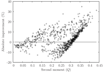
Figure 7: The difference of the maximum success probabilities, in the presence of direction dependent loss with coefficients $\{\eta\}$, and in the presence of uniform loss with coefficient $\eta_{\mathrm{max}}=\max\{\eta\}$. Physically, the non-uniform case can be obtained from the uniform case by introducing proper attenuation. We use the second moment $Q$ as a measure of deviation from the non-attenuated case. The vertical axis shows $[p_{n}^{\mathrm{max}}(\{\eta\})-p_{n}^{\mathrm{max}}(\eta_{\mathrm{max}})]/p_{n}^{\mathrm{max}}(\eta_{\mathrm{max}})$ as a percentage. We observe a systematic improvement for higher values of $Q$. The plot corresponds to rank $n=7$ and $\eta_{\mathrm{max}}=0.996\pm 0.001$.

The numerical studies, involving the generation of 1000 sets of uniformly randomly generated transmission coefficients for each of the systems of up to sizes $n=10$, indicate that with the help of Eq. (34) the first two terms of the expansion Eq. (33) can be used to obtain a general lower bound:

$$p_{n}^{\textrm{max}}(\{\eta\})\geq p_{n}^{\mathrm{max}}(\left<\eta\right>)+2^{-n}Q^{2}.$$ (35)

The inequality implies that the overall contribution from higher order terms is positive, or always balanced by the increase of $B$. The appeal of this lower bound is that it depends only on the size of the system $N=2^{n}$, and the elementary statistical properties of the noise ($\left<\eta\right>$, $Q$). Therefore, together with the formula (20) for uniform loss, a straight-forward estimation of success probability is possible before carrying out an experiment.

Up to now, we concentrated on comparing the performance of the search algorithm suffering non-uniform losses with those suffering uniform loss with coefficient equal to the average of the non-uniform distribution. Another physically interesting question is how attenuation alone affects search efficiency. We can formulate this question using the notations above as follows. Consider a randomly generated distribution $\{\eta\}$ and compare the corresponding success probability with the one generated by a uniform distribution with transmission coefficient $\eta_{\mathrm{max}}=\max\{\eta\}$. We chose $Q$ as a measure of how much an $\eta_{\mathrm{max}}$ uniform distribution needs to be altered to obtain $\{\eta\}$, and made the comparisons using the same set of samples. A typical plot is presented on Fig. 7. It appears that as we start deviating from the original uniform distribution, an initial drop of efficiency is followed by a region where improvement shows some systematic increase. However, it is still an open question, whether it is really a general feature that for some values of $Q$ the efficiency is always increased. On the other hand these plots provide clear evidence that for a significant number of cases the difference $p_{n}^{\mathrm{max}}(\{\eta\})-p_{n}^{\mathrm{max}}(\eta_{\mathrm{max}})$ is positive. In other words, rather counter-intuitively, we can observe examples where increased losses result in the improvement of search efficiency. Since the time evolution with losses is non-unitary, the improvement cannot be trivially attributed to the fact that the Grover operator is not the optimal choice for the marked coin.

V Phase errors

In the present section we discuss another type of errors typically arising in optical multiport networks. These errors are due to stochastic changes of the optical path lengths relative to what is designated, and manifest as undesired random phase shifts. Depending on how rapidly the phases change, we may work in two complementary regimes. In the “phase fluctuation” regime the phases at each iteration are different. These errors can typically be caused by thermal noise. In the “static phase errors” regime, the undesired phases have slow drift such that on the time scale of an entire run of the quantum algorithm their change is insignificant. The origin of such errors can be optical element imperfections, optical misalignments, or a slow stochastic drift in one of the experimental parameters. Phase errors in the fluctuation regime have been studied in Ref. Košik et al. (2006) for walks on $N$ dimensional lattices employing the generalized Grover or Fourier coin. The impact of a different type of static error on the SKW algorithm has been analyzed in Ref. Li et al. (2006).

To begin the formal treatment, let $F$ denote the operator introducing the phase shifts, and write it as

$$F(\{\varphi\})=\sum_{d,x}e^{i\varphi_{dx}}\left|d,x\right>\!\left<d,x\right|.$$ (36)

This operator is unitary, hence the step operator

$$U(\{\varphi\})=SF(\{\varphi\})C^{\prime},$$ (37)

that depends on the phases $\{\varphi_{dx}|d=0..n-1,x=0..2^{n}-1\}$ is unitary as well. In case of phase fluctuations, at each iteration $t$ we have the parameters $\varphi_{dx}^{(t)}$ such that all $\varphi_{dx}^{(t)}$ are independent random variables for every $d$, $x$ and $t$, according to some probability distribution. In case of static phase errors, $\varphi_{dx}^{(t)}$ and $\varphi_{dx}^{(t^{\prime})}$ are considered to be the same random variables for every pair of $d$ and $x$.

The formalism of Ref. Košik et al. (2006) can be applied to the walk on the hypercube, and extended to the case of non-uniform coins and position dependent phases. Namely, using the shorthand notations $D=\left\{0,1,2,\ldots,n-1\right\}$ and

$$E(k,l)=\bigoplus_{j=l}^{k}e_{a_{j}},$$ (38)

the state after $t$ iterations can be expressed as

$$\left|\psi(\{\varphi\},t)\right>=\frac{1}{\sqrt{n2^{n}}}\sum_{x_{0}\in V}(-1)^{\delta_{x_{\mathrm{t}}x_{0}}}\sum_{\underline{a}\in D^{t}}e^{i\varphi(\underline{a},x_{0})}\\ \times\tilde{\Xi}_{x_{\mathrm{t}}}(\underline{a},x_{0})\left|a_{1},x_{0}\oplus E(t,1)\right>,$$ (39)

where

$$\tilde{\Xi}_{x_{\mathrm{t}}}(\underline{a},x_{0})=\\ \prod_{j=1}^{t-1}\left(C^{(0)}_{a_{j}a_{j+1}}+[C^{(1)}-C^{(0)}]_{a_{j}a_{j+1}}\delta_{x_{\mathrm{t}}\oplus x_{0},E(t,j+1)}\right),$$ (40)

and $\varphi(\underline{a},x_{0})=\sum_{j=1}^{t}\varphi^{(t+1-j)}_{a_{j},x_{0}\oplus E(t,j-1)}$. For the standard SKW algorithm, the coin matrices are $C^{(0)}_{aa^{\prime}}=2/n-\delta_{aa^{\prime}}$ and $C^{(1)}_{aa^{\prime}}=-\delta_{aa^{\prime}}$, however, the SKW algorithm is reported to work with more general choices of operators $C_{0/1}$ Shenvi et al. (2003).

For the following study, we express the probability of finding the walker at position $x$ after $t$ iterations as the sum $p_{n}(x,\{\varphi\},t)=p_{n}^{I}(x,\{\varphi\},t)+p_{n}^{C}(x,\{\varphi\},t)$, such that the incoherent and coherent contributions are

$$p_{n}^{I}(x,\{\varphi\},t) = \frac{1}{n2^{n}}\sum_{\underline{a}\in D^{t}}\left|\tilde{\Xi}_{{\tilde{x}}_{\mathrm{t}}}(\underline{a})\right|^{2},$$ (41)

$$p_{n}^{C}(x,\{\varphi\},t) = \frac{1}{n2^{n}}\sum_{\underline{a}\neq\underline{a}^{\prime}}\Phi_{\underline{a}^{\prime}}^{*}\Phi_{\underline{a}}\tilde{\Xi}_{{\tilde{x}}_{\mathrm{t}}}(\underline{a}^{\prime})^{*}\tilde{\Xi}_{{\tilde{x}}_{\mathrm{t}}}(\underline{a})\delta_{a_{1}^{\prime}a_{1}},$$ (42)

where ${\tilde{x}}_{\mathrm{t}}=x_{\mathrm{t}}\oplus x$. The appearing phase factors are

$$\Phi_{\underline{a}}=(-1)^{\delta_{{\tilde{x}}_{\mathrm{t}},E(t,1)}}e^{i\varphi(\underline{a},x\oplus E(t,1))},$$ (43)

and $\tilde{\Xi}_{{\tilde{x}}_{\mathrm{t}}}(\underline{a})=\tilde{\Xi}_{{\tilde{x}}_{\mathrm{t}}}(\underline{a},E(t,1))$, i.e.

$$\tilde{\Xi}_{{\tilde{x}}_{\mathrm{t}}}(\underline{a})=\prod_{j=1}^{t-1}\left(C^{(0)}_{a_{j}a_{j+1}}+[C^{(1)}-C^{(0)}]_{a_{j}a_{j+1}}\delta_{{\tilde{x}}_{\mathrm{t}},E(j,1)}\right).$$ (44)

Note, that when the probability of finding the walker at the target node $x_{\mathrm{t}}$ is to be calculated we must set $x=x_{\mathrm{t}}$, therefore, we have ${\tilde{x}}_{\mathrm{t}}=0$.

In the following we shall show that the incoherent contribution is constant,

$$p_{n}^{I}(x,\{\varphi\},t)=\frac{1}{2^{n}},$$ (45)

for any two unitary coins $C_{0/1}$. Consequently, $p_{n}^{I}$ is constant also for balanced coins such as those in Eq. (5). The summations in Eq. (41) can be rearranged in increasing order of indices of $a_{j}$, yielding

$$p_{n}^{I}(x,\{\varphi\},t)=\\ \frac{1}{n2^{n}}\sum_{a_{1},a_{2}=0}^{n-1}\left|C^{(0)}_{a_{1}a_{2}}+[C^{(1)}-C^{(0)}]_{a_{1}a_{2}}\delta_{{\tilde{x}}_{\mathrm{t}},e_{a_{1}}}\right|^{2}\times\cdots\\ \times\sum_{a_{t-1}=0}^{n-1}\left|C^{(0)}_{a_{t-2}a_{t-1}}+[C^{(1)}-C^{(0)}]_{a_{t-2}a_{t-1}}\delta_{{\tilde{x}}_{\mathrm{t}},E(t-2,1)}\right|^{2}\\ \times\sum_{a_{t}=0}^{n-1}\left|C^{(0)}_{a_{t-1}a_{t}}+[C^{(1)}-C^{(0)}]_{a_{t-1}a_{t}}\delta_{{\tilde{x}}_{\mathrm{t}},E(t-1,1)}\right|^{2}.$$ (46)

Since $E(t-1,1)$ depends on $a_{j}$ only when $j\leq t-1$, and due to the unitarity of the coins $\langle a_{t-1}|C_{0}^{{\dagger}}C_{0}|a_{t-1}\rangle=\langle a_{t-1}|C_{1}^{{\dagger}}C_{1}|a_{t-1}\rangle=1$, the summation over $a_{t}$ can be evaluated and we obtain $1$. Hence, we see that $p_{n}^{I}(x,\{\varphi\},t)=p_{n}^{I}(x,\{\varphi\},t-1)$, and this implies Eq. (45) by induction.

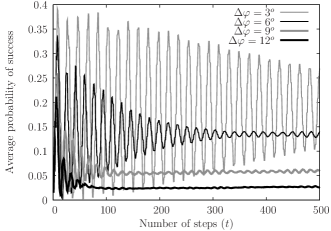
Figure 8: The averaged (1000 samples) probability of measuring the target node, when $n=6$ and $\Delta\varphi=3^{o},6^{o},9^{o},12^{o}$. The tendency of the success probability to a constant, non-zero value can be observed on this numerically obtained plot. It is also observable that a larger variance results in a smaller asymptotic value.

The average probability $\bar{p}_{n}(x,t)$ of finding the walker at node $x$ is obtained by averaging the random phases according to their appropriate probability distribution. Using Eq. (45) this probability can be expressed as

$$\bar{p}_{n}(x,t)=\left<p_{n}(x,\{\varphi\},t)\right>=\frac{1}{2^{n}}+\left<p_{n}^{C}(x,\{\varphi\},t)\right>,$$ (47)

where $\left<\ldots\right>$ denotes taking the average for each random variable $\varphi^{(t)}_{dx}$ in case of phase fluctuations, and for each $\varphi_{dx}$ in case of static phase errors. It is reasonable to assume that each random variable has the same probability distribution. To analyze the impact of phase errors on the search efficiency, we study the behaviour of the coherent term $\left<p_{n}^{C}(x,\{\varphi\},t)\right>$ for different random distributions.

In case of phase fluctuations characterized by a uniform distribution, the coherent term immediately vanishes and we obtain $\bar{p}_{n}(x,t)=1/2^{n}$. This case can be considered as the classical limit of the quantum walk. Therefore, we conclude that the classical limit of the SKW algorithm is not a search algorithm, independently of the two unitary coins used.

Assuming a Gaussian distribution of random phases is motivated by the relation of each phase variable $\varphi$ to the optical path length. The changes in the optical path lengths which introduce phase shifts are not restricted to a $2\pi$ interval. In what follows, we assume that the random phases have a zero centered Gaussian distribution with a variance $\Delta\varphi$.

We arrive at the classical limit even when the phase fluctuations have a finite width Gaussian distribution, simply by repeatedly applying the time evolution operator $U\{\varphi\}$. For such Gaussian distribution, the coherent term exhibits exponential decrease with time, a behaviour also confirmed by our numerical calculations.

In the static phase error regime the mechanism of cancellation of phases is different than in the fluctuation regime, and more difficult to study analytically. For uniform random distribution we expect a sub-exponential decay of the coherent term to zero. For a zero centered Gaussian distribution with variance $\Delta\varphi$ we performed numerical simulations using the standard two coins of Eq. (5).

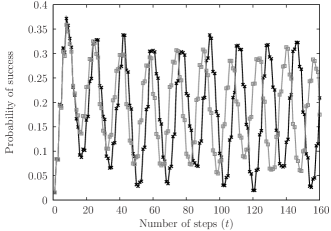
Figure 9: Time dependence of success probabilities for two different phase configurations, numerically calculated for a system of rank $n=6$. The difference in frequencies of the major oscillations is clearly observable for larger times.

The numerical results for the success probability $\bar{p}_{n}(x_{\mathrm{t}},t)$ for several values of $\Delta\varphi$ are plotted on Fig. 8. The data points were obtained by calculating success probabilities for $1000$ randomly generated phase configurations and taking their averages at each time step $t$.

By studying the repetition of the random phase configuration we come to several remarkable conclusions. First, the time evolution of the success probability tends (on a long time scale, $t\gg t_{f}$) to a finite, non-zero constant value. Consequently, being subject to static phase errors, the SKW algorithm retains its utility as search algorithm. Second, the early steps of the time evolution are characterized by damped oscillations reminding of a collapse. Third, the smaller the phase noise the larger is the long time stationary value to which the system evolves. We have plotted the stationary values obtained by numerical calculations, against the rank of the hypercube on Fig. 10.

Better insight into the above features can be gained by examining the shape of the individual runs of the algorithm with the given random phase configurations. As it can be seen on Fig. 9, the success probabilities for different runs display the typical oscillations around a non-zero value. They differ slightly in their frequencies depending on the random phases chosen, hence when these oscillations are summed up we get the typical collapse behaviour. Also, since these frequencies continuously fill up a band specified by the width of the Gaussian, we expect no revivals to happen later. For higher order hypercubes the success probability drops almost to zero for already very moderate phase errors, resembling a behaviour seen on Fig. 3.

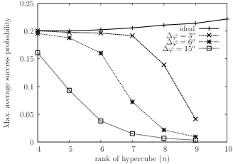
Figure 10: The long time stationary values of the success probability (obtained by averaging over 1000 samples) against the size of the search space, for $\Delta\varphi=0^{o},3^{o},6^{o},15^{o}$.

VI Conclusions

We studied the SQRW implementation of the SKW search algorithm and analyzed the influence on its performance the two most common type of disturbances, namely photon losses and phase errors. Our main result for the photon loss affected SQRW search algorithm is that the introduction of non-uniform distribution of the loss can significantly improve the search efficiency compared to uniform loss with the same average. In many cases, even the sole increase of losses in certain directions may improve the search efficiency. Mostly based on numerical evidence we have set a lower bound for the search probability as a function of the average and variance of the randomly distributed direction dependent loss.

We concentrated our analysis on two complementary regimes of phase errors. When the system is subject to rapid phase fluctuations, the classical limit of the quantum walk is approached. We have shown that in this limit the SKW algorithm loses its applicability to the search problem for any pair of unitary coins. On the other hand, we showed that when the phases are kept constant during each run of the search, the success rate does not drop to zero, but approaches a finite value. The effect in its mechanism is reminiscent to exponential localization found in optical networks Törmä et al. (2002). Therefore, in the long-time limit, static phase errors are less destructive than rapidly fluctuating phase errors.