Spontaneous decay of an excited atom placed near a rectangular plate

Abstract

Using the Born expansion of the Green tensor, we consider the spontaneous decay rate of an excited atom placed in the vicinity of a rectangular plate. We discuss the limitations of the commonly used simplifying assumption that the plate extends to infinity in the lateral directions and examine the effects of the atomic dipole moment orientation, atomic position, and plate boundary and thickness on the atomic decay rate. In particular, it is shown that in the boundary region, the spontaneous decay rate can be strongly modified.

The ability to control the spontaneous decay process holds the key to powerful applications in micro- and nano-optical devices. Effective control can be achieved by tailoring the environment surrounding the emitters. In theoretical analysis of surrounding environment of different geometries, the most interesting ones being of the resonator type, the boundary conditions are typically taken into account only in directions in which the electromagnetic field is confined or affected the most. For example, in a planar configuration, only the boundary conditions in the normal direction are taken into account while those in the lateral directions are neglected (see, e.g., Ref. Chance78 ). In a cylindrical configuration that extends to infinity, the reverse is true Erdogan93 . Under appropriate conditions, these approximations are generally valid. However, as the sizes of devices decrease and fall in the micro- and nano-meter ranges as in the current trend of miniaturization, it is clearly of great importance to keep track of the effects of all boundaries. One way to calculate the spontaneous decay rate in an arbitrary geometry is to directly solve the Maxwell equations using the finite difference time domain method Xu00 . This method, which relies entirely on numerical computation, is not without weaknesses. It requires that the whole computational domain be gridded, leading to very large computational domains in cases of extended geometries, or in cases where the field values at some distance are required. All curved surfaces must be modelled by a stair-step approximation, which can introduce errors in the results. Additionally, the discretization in time may be a source of errors in the longitudinal field Xu00 .

Here we employ an approach that, in a sense, combines analytical and numerical calculations, thereby significantly reducing the numerical computation workload. This approach relies on first writing the atomic decay rate in terms of the Green tensor characterizing the surrounding media Agarwal75 ; Ho00 . Although this formula holds for arbitrary boundary conditions, exact analytical evaluation of the Green tensors for realistic, finite-size systems can be very cumbersome or even prohibitive. Following Buhmann06 and Ho06 , where the atom-body van der Waals force and the local-field correction, respectively, have been considered, we circumvent the task of an exact calculation of the Green tensor by writing it in terms of a Born series and restrict ourselves to leading-order terms. The boundary conditions enter the theory only via the integral limits. This approach is universal in the sense that it works for an arbitrary geometry of the surrounding media, and can be used to evaluate any characteristics of the matter-electromagnetic field interaction expressible in terms of the Green tensor. In this paper, we are concerned mostly with the spontaneous decay rate of an excited atom placed near a rectangular plate. Our aim is twofold: first, we compare our results with those for an infinitely extended plate in order to establish in a quantitative way the conditions under which the approximation of an infinitely extended plate is valid; second, we examine the effects brought about by the presence of the boundaries in the lateral directions.

The (classical) Green tensor of an arbitrary dispersing and absorbing body satisfies the equation

$$\hat{H}{\bm{G}}({\bf r},{\bf r}^{\prime},\omega)=\delta({\bf r}-{\bf r}^{\prime})\bm{I},$$ (1)

$$\hat{H}({\bf r})\equiv\bm{\nabla}\times\frac{1}{\mu({\bf r},\omega)}\bm{\nabla}\times-\frac{\omega^{2}}{c^{2}}\,\varepsilon({\bf r},\omega),$$ (2)

($\bm{I}$-unit tensor) together with the boundary condition at infinity, where $\varepsilon({\bf r},\omega)$ [$\mu({\bf r},\omega)$] is the frequency- and space-dependent complex permittivity (permeability) which obeys the Kramers-Kronig relations.

Decomposing the permittivity and permeability as

$$\varepsilon({\bf r},\omega)=\bar{\varepsilon}({\bf r},\omega)+\chi_{\varepsilon}({\bf r},\omega),\ \ \mu({\bf r},\omega)=\bar{\mu}({\bf r},\omega)+\chi_{\mu}({\bf r},\omega),$$ (3)

and assuming that the solution $\bar{\bm{G}}({\bf r},{\bf r}^{\prime},\omega)$ to the equation $\hat{\bar{H}}({\bf r})\bar{\bm{G}}({\bf r},{\bf r}^{\prime},\omega)=\delta({\bf r}-{\bf r}^{\prime})\bm{I},$ where $\hat{\bar{H}}$ is defined as in Eq. (2) with $\bar{\varepsilon}$ instead of $\varepsilon$ and $\bar{\mu}$ instead of $\mu$, is known, the Green tensor $\bm{G}$ can be written as

$$\bm{G}(\mathbf{r},\mathbf{r}^{\prime},\omega)=\bar{\bm{G}}(\mathbf{r},\mathbf{r}^{\prime},\omega)+\bm{G}^{\prime}(\mathbf{r},\mathbf{r}^{\prime},\omega).$$ (4)

Substituting Eq. (4) into Eq. (1) and using the identity $(\bar{\mu}+\chi_{\mu})^{-1}=\bar{\mu}^{-1}\sum_{l=0}^{\infty}(\chi_{\mu}/\bar{\mu})^{l}$, it can be found that

$$\hat{H}({\bf r})\bm{G}^{\prime}(\mathbf{r},\mathbf{r}^{\prime},\omega)=\hat{H}_{\chi}({\bf r})\bar{\bm{G}}(\mathbf{r},\mathbf{r}^{\prime},\omega)\equiv\tilde{\bm{G}}(\mathbf{r},\mathbf{r}^{\prime},\omega)$$ (5)

$$\hat{H}_{\chi}({\bf r})\equiv-\bm{\nabla}\times\frac{1}{\bar{\mu}({\bf r},\omega)}\sum_{l=1}^{\infty}\frac{\chi^{l}_{\mu}({\bf r},\omega)}{\bar{\mu}^{l}({\bf r},\omega)}\bm{\nabla}\times+\frac{\omega^{2}}{c^{2}}\chi_{\varepsilon}({\bf r},\omega),$$ (6)

i.e., $\bm{G}^{\prime}$ satisfies the same differential equation as the one governing the electric field, with the current being equal to $\tilde{\bm{G}}$. Hence it can be written as a convolution of this current with the kernel $\bm{G}$: $\mathbf{G^{\prime}}(\mathbf{r},\mathbf{r}^{\prime},\omega)=\int d^{3}s\bm{G}(\mathbf{r},\mathbf{s},\omega)\tilde{\bm{G}}(\mathbf{s},\mathbf{r}^{\prime},\omega)\,.$ Substitution of $\bm{G}^{\prime}$ in this form in Eq. (4) and iteration lead to the desired Born series

$$\bm{G}({\bf r},{\bf r}^{\prime},\omega)=\bar{\bm{G}}({\bf r},{\bf r}^{\prime},\omega)+\sum_{k=1}^{\infty}\bm{G}_{k}({\bf r},{\bf r}^{\prime},\omega),$$ (7)

$$\bm{G}_{k}({\bf r},{\bf r}^{\prime},\omega)=\Biggl{(}\prod_{j=1}^{k}\int\mathrm{d}^{3}s_{j}\Biggr{)}$$

$$\quad\times\bar{\bm{G}}({\bf r},{\bf s}_{1},\omega)\tilde{\bm{G}}({\bf s}_{1},{\bf s}_{2},\omega)\cdots\tilde{\bm{G}}({\bf s}_{k},{\bf r}^{\prime},\omega)\,.$$ (8)

This formal expansion for the Green tensor is valid for an arbitrary geometry, permittivity, and permeability of the macroscopic bodies. Obviously, one of the situations in which the Born series is particularly useful is when $\chi_{\varepsilon}$ is a perturbation to $\bar{\varepsilon}$ and $\chi_{\mu}$ is a perturbation to $\bar{\mu}$, thereby one makes only a small error cutting off higher-order terms. For such weakly dielectric and magnetic bodies, it is natural to choose

$$\bar{\varepsilon}({\bf r},\omega)=\bar{\mu}({\bf r},\omega)=1$$ (9)

with $\chi_{\lambda}({\bf r},\omega)$ $\!=$ $\!\chi_{\lambda{\rm R}}({\bf r},\omega)+i\chi_{\lambda{\rm I}}({\bf r},\omega)$, $|\chi_{\lambda}({\bf r},\omega)|\ll 1$ $(\lambda=\varepsilon,\ \mu)$ [cf. Eqs. (3)]. This implies we restrict ourselves to frequencies far from a medium resonance.

The Green tensor $\bar{\bm{G}}$ corresponding to $\bar{\varepsilon}({\bf r},\omega)=\bar{\mu}({\bf r},\omega)=1$ is the vacuum Green tensor

$$\bar{\bm{G}}({\bf r},{\bf r}^{\prime},\omega)=-\frac{\delta({\bf u})}{3k^{2}}\bm{I}+\frac{k}{4\pi}(a\bm{I}-b\hat{{\bf u}}\otimes\hat{{\bf u}})e^{iq},$$ (10)

$$a\equiv a(q)=\frac{1}{q}+\frac{i}{q^{2}}-\frac{1}{q^{3}},\quad b\equiv b(q)=\frac{1}{q}+\frac{3i}{q^{2}}-\frac{3}{q^{3}}$$ (11)

($k$ $\!=$ $\omega/c$; ${\bf u}$ $\!\equiv$ $\!{\bf r}-{\bf r}^{\prime}$; $\hat{{\bf u}}={\bf u}/u$, and $q$ $\!\equiv$ $ku$).

A description of quantities such as the emission pattern or the interatomic van der Waals forces requires the knowledge of the Green tensor of different positions, while a description of quantities such as the spontaneous decay rate of an excited atom or the atom-body van der Waals forces requires the knowledge of the Green tensor of equal positions. Substituting Eq. (10) in Eq. (Spontaneous decay of an excited atom placed near a rectangular plate) and assuming that the position ${\bf r}$ lies outside the region occupied by the macroscopic bodies, we derive for the first-order term in the Born expansion of the equal-position Green tensor

$$\bm{G}_{1}({\bf r},{\bf r},\omega)=\frac{k^{2}}{16\pi^{2}}\int\mathrm{d}^{3}s\,\hat{H}_{\chi 1}({\bf s})$$

$$\quad\times[a^{2}\bm{I}+(b^{2}-2ab)\hat{{\bf u}}\otimes\hat{{\bf u}}]e^{2iq}$$ (12)

[${\bf u}$ $\!\equiv$ $\!{\bf r}-{\bf s}$; $q=ku$; $a$ $\!=$ $\!a(q)$; $b$ $\!=$ $\!b(q)$; $\hat{H}_{\chi 1}({\bf r})\equiv-\bm{\nabla}\times\chi_{\mu}({\bf r},\omega)\bm{\nabla}\times+\frac{\omega^{2}}{c^{2}}\chi_{\varepsilon}({\bf r},\omega)$ – linear part of $\hat{H}_{\chi}$, Eq. (6)]. Higher-order terms can easily be obtained by repeatedly using Eq. (10) in Eq. (Spontaneous decay of an excited atom placed near a rectangular plate).

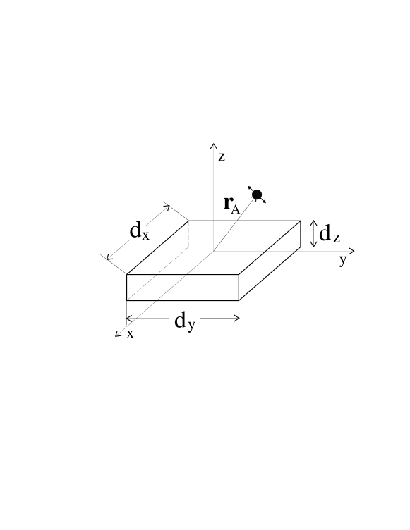
Figure 1: A dipole emitter in the vicinity of a rectangular plate.

Our system consists of an excited two-level atom surrounded by macroscopic media, which can be absorbing and dispersing. In the electric-dipole and rotating-wave approximations, the atomic decay rate reads as Agarwal75 ; Ho00

$$\Gamma=\frac{2k_{\rm A}^{2}}{\hbar\varepsilon_{0}}\,{\bf d}_{\rm A}{\rm Im}\,{\bm{G}}({\bf r}_{\rm A},{\bf r}_{\rm A},\omega_{\rm A}){\bf d}_{\rm A},$$ (13)

where ${\bf d}_{\rm A}$ and $\omega_{\rm A}$ are the atomic dipole and shifted transition frequency, $k_{\rm A}=\omega_{\rm A}/c$, and ${\bm{G}}$ is the Green tensor describing the surrounding media.

Figure 2: Atom-surface distance dependence of the normalized spontaneous decay rate of an excited atom positioned at ($0,0,z_{\rm A}$) near an infinite planar plate (solid line) and a rectangular plate ($d_{x}=d_{y}=10\lambda_{\rm A}$, dashed line) of equal thickness $d_{z}=0.2\lambda_{\rm A}$ and equal $\chi_{\varepsilon}=\chi_{\varepsilon{\rm R}}+i10^{-8}$. Case (a) is for a $x$-oriented dipole moment, while case (b) is for a $z$-oriented dipole moment.

In accordance with the linear Born expansion, Eqs. (7), (10), and (Spontaneous decay of an excited atom placed near a rectangular plate) yield, for a purely electric material,

$$\frac{\Gamma^{\parallel(\bot)}}{\Gamma_{0}}=1+\frac{3k_{\rm A}^{3}}{8\pi}{\rm Im}\Biggl{\{}\int\mathrm{d}^{3}s\,\chi_{\varepsilon}({\bf s},\omega_{\rm A})$$

$$\times\biggl{[}a^{2}+(b^{2}-2ab)\frac{1}{u^{2}}{(x-x_{\rm A})^{2}\atop(z-z_{\rm A})^{2}}\biggr{]}e^{2iq}\Biggr{\}}$$ (14)

[$\Gamma_{0}=k_{\mathrm{A}}^{3}d_{\mathrm{A}}^{2}/(3\pi\hbar\varepsilon_{0})$ - free-space decay rate, ${\bf s}=(x,y,z)$, $u=|{\bf s}-{\bf r}_{\rm A}|$, $q=k_{\rm A}u$, $a=a(q)$, $b=b(q)$] for $x$-($z$-)oriented dipole moments. Equations (Spontaneous decay of an excited atom placed near a rectangular plate) are our main working equations. Just like the Born expansion of the Green tensor, they hold for an arbitrary geometry of the surrounding environment.

Next let us be specific about the shape of the macroscopic bodies. We consider a rectangular plate of dimensions $d_{x}$, $d_{y}$, and $d_{z}$ and choose a Cartesian coordinate system such that its origin is located at the center of one surface of the plate, as sketched in Fig. 1. Then $\Gamma^{\parallel}$ represents the spontaneous decay rate of a dipole moment parallel to a plate surface and $\Gamma^{\bot}$ – that of a dipole moment normal to the same surface. Since no further analytical calculation in Eqs. (Spontaneous decay of an excited atom placed near a rectangular plate) seems possible, we resort to numerical computation.

In Fig. 2 we present the spontaneous decay rate in accordance with the linear Born expansion (Spontaneous decay of an excited atom placed near a rectangular plate), as a function of the atom-surface distance for two different values of the permittivity. The same quantity but for an atom placed near an infinitely extended planar slab is plotted using the Green tensor given in Ref. Tomas95 . It can be seen that when the lateral dimensions of the rectangular plate are sufficiently large and the absolute value of the permittivity is sufficiently close to one (the case of $\chi_{\varepsilon}=0.1+i10^{-8}$ in the figure), the two results almost coincide for both dipole moment orientations. As $\chi_{\varepsilon{\rm R}}$ increases, the agreement worsens but is still quite good at $\chi_{\varepsilon{\rm R}}=0.5$. Further numerical calculations indicate that in the range of $|\chi_{\varepsilon}(\omega_{\rm A})|\stackrel{{\scriptstyle<}}{{\sim}}0.5$, the spontaneous decay rate can be well approximated by the linear Born expansion. In Fig. 2, the atom has been moved along the $z$-axis with $x_{\rm A}=y_{\rm A}=0$. When the atom is moved along other lines parallel to the $z$-axis but nearer to the border, the $z_{\rm A}$-dependence of the normalized spontaneous decay rates behaves in a similar way as in Fig. 2 but with its value being generally closer to one. Having determined the range of permittivities where the linear Born expansion provides a good approximation to the spontaneous decay rate, we move on now to investigate when the plate can be regarded as an infinite slab.

Figure 3: The same as in Fig. 2 but for different sizes of the rectangular plate: $d_{x}=d_{y}=3\lambda_{\rm A}$ (dashed line), $0.4\lambda_{\rm A}$ (dotted line), and $0.2\lambda_{\rm A}$ (dash-dotted line). In the last case, the plate is actually a cube. The curves for an infinite planar plate are shown by solid line and $\chi_{\varepsilon}=0.1+i10^{-8}$.

Figure 4: Plate-thickness dependence of the spontaneous decay rate of an excited atom located near an infinitely extended planar plate (solid line) and a rectangular plate ($d_{x}=d_{y}=10\lambda_{\rm A}$, dashed line) of equal $\chi_{\varepsilon}=0.1+i10^{-8}$. The atomic position is fixed at (0,0,$0.2\lambda_{\rm A}$) in the main figure, and (0,0,$5\lambda_{\rm A}$) in the inset.

In Fig. 3, we gradually reduce the lateral sizes of the rectangular plate while keeping its thickness constant, and compare the resulting spontaneous decay rates with that for an infinite slab. To be on the conservative side, the permittivity is set equal to $\varepsilon(\omega_{\rm A})=1.1+i10^{-8}$ – a value which is very close to one (cf. Fig. 2). For lengths of the lateral sides comparable to the atomic transition wavelength, the infinite slab approximation starts to differ noticeably from the linear Born expansion (see the figure, case of $d_{x}=d_{y}=3\lambda_{\rm A}$), which in this situation is regarded as a good and nondegrading approximation. As the lateral sizes of the plate decrease further and become smaller than $\lambda_{\rm A}$, the infinite-slab approximation fails completely (see cases of $d_{x}=d_{y}=0.4\lambda_{\rm A}$ and $0.2\lambda_{\rm A}$ in the figure). In other words, while a rectangular plate with lateral sizes much larger than the atomic transition wavelength can be more or less treated as an infinite slab, care should be taken when the sizes are reduced to about or below a wavelength. This happens for both normal and parallel to the surface dipole moment orientations. When the rectangular plate can be roughly regarded as an infinite slab, the infinite-slab curve and the linear Born expansion curve agree better when the atom is placed closer to the surface (see dashed and solid curves in the figure). This can be explained by that the closer to the surface the atom is situated, the more it is inclined to see the plate as infinite.

Figure 5: Effects of the presence of a boundary in the $x$-direction on the spontaneous decay rate of an excited atom located near a rectangular plate of permittivity $\varepsilon(\omega_{\rm A})=1.5+i10^{-8}$ and dimensions $d_{z}=0.2\lambda_{\rm A}$ and $d_{x}=d_{y}=10\lambda_{\rm A}$. The atom is located at ($x_{\rm A}$,0, $0.01\lambda_{\rm A}$).

Besides the dependence on the lateral sizes, whether a rectangular plate can be treated as an infinitely extended one clearly depends on its thickness as well. It is intuitively obvious that even when plate lateral sizes are much larger than the atomic transition wavelength, the plate cannot be treated as extending to infinity if its thickness is comparable with the lateral sizes. In Fig. 4, we compare the $d_{z}$-dependence of the spontaneous decay rate for a rectangular plate with that for an infinite slab. The agreement between the two curves, being very good for sufficiently thin plates, gradually worsens with an increasing plate thickness. The disagreement is already noticeable at $d_{z}\sim\lambda_{\rm A}$ – a value which is still much smaller than the lateral sizes $d_{x}=d_{y}=10\lambda_{\rm A}$, and it sets in earlier for $\Gamma^{\bot}$ than for $\Gamma^{\parallel}$. The two calculations predict quite different large-thickness limits. This means that in the case of thick plates, one must take into account the boundary conditions in the lateral directions in order to obtain reliable results.

Account of the boundary conditions in the lateral directions also gives rise to some curious beating in the $d_{z}$-dependence of the spontaneous decay rate, which is especially visible when the atom has a dipole moment oriented parallel to the surface and is situated somewhat away from the surface (see Fig. 4, inset). Let’s have a closer look at, say, the decay rate for a dipole oriented parallel to the surface. Using the stationary phase method, one obtains from Eq. (Spontaneous decay of an excited atom placed near a rectangular plate)

$$\frac{\Gamma^{\parallel}}{\Gamma_{0}}\simeq 1+\frac{3k_{\rm A}^{3}}{2\pi}{\rm Im}\Biggl{[}\chi_{\varepsilon}\int_{0}^{d_{z}}{\rm d}za^{2}(q_{z})e^{2iq_{z}}$$

$$\times\int_{0}^{\frac{d_{x}}{2}}{\rm d}x\int_{0}^{\frac{d_{y}}{2}}{\rm d}y\,e^{i\frac{k_{\rm A}^{2}}{q_{z}}(x^{2}+y^{2})}\Biggr{]}$$ (15)

[$q_{z}=k_{\rm A}(z+z_{\rm A})$]. The integrals over $x$ and $y$ in Eq. (Spontaneous decay of an excited atom placed near a rectangular plate) contain Fresnel integrals. In the limit of an infinite plate $d_{x},\ d_{y}\rightarrow\infty$, Eq. (Spontaneous decay of an excited atom placed near a rectangular plate) becomes

$$\frac{\Gamma^{\parallel}}{\Gamma_{0}}\simeq 1+\frac{3k_{\rm A}}{16}{\rm Im}\Biggl{[}\chi_{\varepsilon}\int_{0}^{d_{z}}{\rm d}za^{2}(q_{z})q_{z}e^{2iq_{z}}(1+i)^{2}\Biggr{]}.$$ (16)

As a function of $z/\lambda_{\rm A}$, the integrand in Eq. (16) has a period of $\frac{1}{2}$. Since this period is $z$-independent, the resulting integral must exhibit oscillations with the same period, as confirmed by Fig. 4, solid curves. These oscillations survive for plates of finite lateral extensions (Fig. 4, dashed curves). The beating clearly arises from the finite values of $d_{x}$ and $d_{y}$. Note that as a function of $z$, the inner integrands in Eq. (Spontaneous decay of an excited atom placed near a rectangular plate) have a ‘period’ that is $z$- dependent and that increases with increasing $z$.

Next we turn to elucidating the influence of the boundaries in the $x$- and $y$-directions on the spontaneous decay rates. As can be seen from Fig. 5, where an edge is present at $x_{\rm A}=5\lambda_{\rm A}$, the decay rates exhibit oscillations near the boundary with a particularly strong magnitude right on either side of it, and damping tails. The oscillations are more pronounced for a dipole moment oriented parallel to the ($xy$)-plane than for a $z$-oriented dipole moment. One can notice that when the projection of the atomic position on the $xy$-plane lies outside and sufficiently far from the boundaries, the spontaneous decay rate approaches one in free space, as it should.

In summary, using the Born expansion of the Green tensor, we have considered the decay rate of an atom located near a plate of rectangular shape. We have shown that a rectangular plate can be treated as extending to infinity only when its lateral sizes are much larger than the atomic transition wavelength, its thickness sufficiently small, and the atom is located close enough to the plate surface. We have also shown that a boundary in the lateral directions can give rise to significant modifications of the decay rate in either side of it. The first-order Born expansion remains quite reliable even at a value of permittivity as high as 1.5. Inclusion of higher-order terms would allow one to investigate more dense media.

H.T.D. thanks S. Y. Buhmann and D.-G. Welsch for enlightening discussions. We are grateful to J. Weiner for a critical reading of the manuscript. This work has been supported by the Ho Chi Minh city National University and the National Program for Basic Research of Vietnam.

References

- (1) R. R. Chance, A. Prock, and R. Silbey, in Advances in Chemical Physics, edited by I. Prigogine and S. A. Rice (Wiley, New York, 1978), Vol. 37, p. 1; Ho Trung Dung and K. Ujihara, Phys. Rev. A 60, 4067 (1999).
- (2) T. Erdogan, K. G. Sullivan, D. G. Hall, J. Opt. Soc. Am. B 10, 391 (1993); H. Nha and W. Jhe, Phys. Rev. A 56, 2213 (1997); W. Żakowicz and M. Janowicz ibid. 62, 013820 (2000).
- (3) Y. Xu, R. K. Lee, and A. Yariv, Phys. Rev. A 61, 033807 (2000); ibid., 033808 (2000).
- (4) G. S. Agarwal, Phys. Rev. A 12, 1475 (1975); J. M. Wylie and J. E. Sipe, Phys. Rev. A 30, 1185 (1984).
- (5) Ho Trung Dung, L. Knöll, and D.-G. Welsch, Phys. Rev. A 62, 053804 (2000).
- (6) S. Y. Buhmann and D.-G. Welsch, Appl. Phys. B: Lasers Opt. 82, 189 (2006).
- (7) Ho Trung Dung, S. Y. Buhmann, and D.-G. Welsch, Phys. Rev. A 74, 023803 (2006).
- (8) M. S. Tomaš, Phys. Rev. A 51, 2545 (1995); W. C. Chew, Waves and Fields in Inhomogeneous Media (IEEE Press, New York, 1995).