Linearity and Quantum Adiabatic Theorem

Abstract

We show that in a quantum adiabatic evolution, even though the adiabatic approximation is valid, the total phase of the final state indicated by the adiabatic theorem may evidently differ from the actual total phase. This invalidates the application of the linearity and the adiabatic approximation simultaneously. Besides, based on this observation we point out the mistake in the traditional proof for the adiabatic theorem. This mistake is the root of the troubles that the adiabatic theorem has met. We also show that a similar mistake remains in some recent modifications of the traditional adiabatic theorem attempting to eliminate the troubles.

The adiabatic theorem BF28 ; LIS55 is an important result in quantum theory, which has a long history. Since discovered, it has been widely applied in various areas of physics such as nuclear physics, quantum field theory and so on. This theorem states that if the the state of a quantum system is governed by a slowly changing Hamiltonian, and if the initial state of this system is one of the eigenstates of the initial Hamiltonian, then the state of the system at any time will be the corresponding eigenstate of the Hamiltonian of that time up to a multiplicative phase factor. About two decades ago, when studying circular adiabatic evolution, Berry discovered a new phenomenon called geometric phase Berry84 , which has been generalized to many other cases AA87 ; SB88 ; Uhl86 ; ES00 . Besides, since quantum information science bloomed, quantum adiabatic theorem has been employed essentially in two very important schemes of quantum computation, namely geometric quantum computation ZR99 ; JVEC00 and quantum adiabatic computation FGGS00 .

On the other hand, adiabatic theorem has been reexamined in the recent years. Some authors MS04 ; TSKO05 ; TSKFO05 noted that one must be careful in employing the adiabatic theorem. Concretely, Marzlin and Sanders demonstrated that a perfunctory application of the theorem may lead to an inconsistency MS04 . Furthermore, Tong et al. pointed out that the root of the inconsistency is that the traditional adiabatic conditions are not sufficient to guarantee the validity of adiabatic approximation TSKO05 . To eliminate the inconsistency, some modified adiabatic conditions have been proposed, such as those in Refs.YZZG05 ; DMN05 ; COM06 .

In this letter, we propose a new approach to revisit quantum adiabatic theorem. We show that, in an adiabatic evolution, even if the adiabatic approximation is valid under some conditions , the total phase indicated by the adiabatic theorem may differ evidently from the actual value. Here, “the validity of the adiabatic approximation” means that the state of the system equals approximatively to some eigenstate of the Hamiltonian up to a phase factor all the time. For convenience, we call the phase of this phase factor total phase. Generally, the global phase of a quantum state is not important from an observational point of view. However, the global phase can be changed to a relative phase when we combine the adiabatic approximation and the linearity, the well-known property of quantum mechanics. Different relative phases may give rise to physically observable differences, so our result points out that the linearity of adiabatic approximation may fail. Therefore, errors in the approximation of phase may lead to severe problems when linearity is also used. On the other hand, by reexamining the adiabatic theorem based on this observation, we reveal the mistake in its traditional proof. It is this mistake that makes the traditional adiabatic conditions not sufficient to guarantee the validity of adiabatic approximation. At last, we show that there are similar problems with some modified adiabatic conditions YZZG05 ; DMN05 .

For convenience of the later presentation, let us recall the quantum adiabatic theorem and its traditional proof.

Suppose we have a quantum system and the evolution of its state $|\psi(t)\rangle(t_{0}\leq t)$ is governed by a time-dependent Hamiltonian $H(t)$. Suppose the initial state $|\psi(t_{0})\rangle=|E_{k}(t_{0})\rangle$ is an eigenstate of the initial Hamiltonian $H(t_{0})$. In the instantaneous eigenbasis ${|E_{n}(t)\rangle}$ of $H(t)$, the state can be expressed as

$$|\psi(t)\rangle=\sum_{n}\psi_{n}(t)e^{-i\int E_{n}}|E_{n}(t)\rangle,$$ (1)

where $\int E_{n}=\int^{t}_{t_{0}}E_{n}(t^{\prime})dt^{\prime}.$ Substituting Eq.(1) into the Schrödinger equation

$$i\frac{d}{dt}|\psi(t)\rangle=H(t)|\psi(t)\rangle,$$ (2)

we obtain the following differential equation:

$$i\dot{\psi_{n}}=-i\sum_{m}e^{i\int(E_{n}-E_{m})}\psi_{m}\langle E_{n}|\dot{E_{m}}\rangle.$$ (3)

If it holds that

$$|\langle E_{n}|\dot{E_{m}}\rangle|\ll|E_{n}-E_{m}|,\ \ n\neq m,$$ (4)

the phase factor $\exp{(i\int(E_{n}-E_{m}))}$ in Eq.(3) will be a rapid oscillation. This can make transitions to other levels negligible, and results in

$$|\psi(t)\rangle\approx e^{-i\int E_{k}}e^{-\int\langle E_{k}|\dot{E_{k}}\rangle}|E_{k}(t)\rangle.$$ (5)

Here we call Eq.(4) the traditional adiabatic conditions. The standard adiabatic theorem states that, if these conditions hold, we have approximation Eq.(5).

One can also prove this theorem as follows. Suppose

$$|e_{i}(t)\rangle=e^{-\int\langle E_{i}|\dot{E_{i}})}|E_{i}(t)\rangle,\ \ i=1,...,N.$$ (6)

In the new instantaneous eigenbasis ${|e_{n}(t)\rangle}$ of $H(t)$, the state can be expressed as ($\psi_{n}$’s are different from those of the above)

$$|\psi(t)\rangle=\sum_{n}\psi_{n}(t)e^{-i\int E_{n}}|e_{n}(t)\rangle.$$ (7)

Substituting Eq.(7) into the Schrödinger equation gives

$$i\dot{\psi_{n}}=-i\sum_{m\neq n}e^{i\int(E_{n}-E_{m})}\psi_{m}\langle e_{n}|\dot{e_{m}}\rangle.$$ (8)

Similarly, if

$$|\langle e_{n}|\dot{e_{m}}\rangle|=|\langle E_{n}|\dot{E_{m}}\rangle|\ll|E_{n}-E_{m}|,\ \ n\neq m,$$ (9)

we know that the integral of the rhs (right hand side) of Eq.(8) is negligible, due to which we get (let $n=k$)

$$\psi_{k}(t)-\psi_{k}(t_{0})\approx 0.$$ (10)

Note that

$$\psi_{k}(t_{0})=1.$$ (11)

We finally get

$$|\psi(t)\rangle\approx e^{-i\int E_{k}}e^{-\int\langle E_{k}|\dot{E_{k}})}|E_{k}(t)\rangle,$$ (12)

which finishes the proof of the traditional adiabatic theorem once more.

From Eq.(5) we know that after an adiabatic evolution, the state of the system has an approximate total phase. Now we show that there may be a significant gap between this approximate total phase and the corresponding exact total phase. To be concrete, we use a simple but interesting example to show this point (See also TSKFO05 ; TSKO05 ).

Let us consider a spin-half particle in a rotating magnetic field. The Hamiltonian of the system can be written as

$$H(t)=-\frac{\omega_{0}}{2}\begin{pmatrix}\cos{\theta}&\sin{\theta}e^{-i\omega t}\\ \sin{\theta}e^{-i\omega t}&-\cos{\theta}\\ \end{pmatrix},$$ (13)

where $\omega_{0}$ is a time-independent parameter defined by the magnetic moment of the spin and the intensity of external magnetic field, $\omega$ is the rotating frequency of the magnetic field. The instantaneous eigenvalues and eigenstates of $H(t)$ are

$$E_{1}=\frac{\omega_{0}}{2},\ \ E_{2}=-\frac{\omega_{0}}{2},$$ (14)

$$|E_{1}(t)\rangle=\begin{pmatrix}e^{-i\omega t/2}\sin{\frac{\theta}{2}}\\ -e^{i\omega t/2}\cos{\frac{\theta}{2}}\\ \end{pmatrix},$$ (15)

$$|E_{2}(t)\rangle=\begin{pmatrix}e^{-i\omega t/2}\cos{\frac{\theta}{2}}\\ e^{i\omega t/2}\sin{\frac{\theta}{2}}\\ \end{pmatrix},$$ (16)

respectively. The adiabatic conditions Eq.(4) are satisfied as long as

$$\omega_{0}\gg\omega\sin{\theta}.$$ (17)

Suppose that the system is initially in the state $|E_{1}(0)\rangle$. At time $t$, according to the adiabatic theorem, the system will be in the instantaneous eigenstate $|E_{1}(t)\rangle$ up to a phase factor. This approximate total phase $\gamma(\tau)$ can be calculated by Eq.(5),

$$\gamma(\tau)=-\int E_{0}+i\int\langle E_{0}|\dot{E_{0}}).$$ (18)

Substituting Eqs.(14)-(16) into Eq.(18) gives

$$\gamma(\tau)=-\frac{\tau}{2}(\omega_{0}+\omega\cos{\theta}).$$ (19)

On the other hand, we can evaluate this total phase almost without any approximation. Let us express the exact state of the system as

$$|\psi(t)\rangle=a(t)|E_{1}(t)\rangle+b(t)|E_{2}(t)\rangle.$$ (20)

By solving the Schrödinger equation it can be checked that

$$a(t)=\cos{\frac{\bar{\omega}t}{2}}-i\frac{\omega_{0}+\omega\cos{\theta}}{\bar{\omega}}\sin{\frac{\bar{\omega}t}{2}},$$ (21)

$$b(t)=i\frac{\omega\sin{\theta}}{\bar{\omega}}\sin{\frac{\bar{\omega}t}{2}},$$ (22)

where $\bar{\omega}=\sqrt{\omega^{2}+\omega_{0}^{2}+2\omega\omega_{0}\cos{\theta}}$.

When the traditional adiabatic condition Eq.(17) is satisfied, $b(t)\rightarrow 0$, so $|\psi(t)\rangle\approx a(t)|E_{1}(t)\rangle$. Then we can regard the exact total phase as

$$\begin{aligned} \hat{\gamma}(\tau)=&\arg{(\cos{\frac{\bar{\omega}\tau}{2}}-i\frac{\omega_{0}+\omega\cos{\theta}}{\bar{\omega}}\sin{\frac{\bar{\omega}\tau}{2}})}\\ \approx&-\frac{\bar{\omega}\tau}{2}.\end{aligned}$$

We finally get

$$\begin{aligned} \gamma(\tau)-\hat{\gamma}(\tau)\approx&\frac{\bar{\omega}\tau}{2}-\frac{\tau}{2}(\omega_{0}+\omega\cos{\theta})\\ =&\frac{1}{2}\cdot\frac{\omega^{2}\sin^{2}{\theta}}{\bar{\omega}+(\omega_{0}+\omega\cos{\theta})}\tau.\end{aligned}$$

That is to say, the difference between $\gamma(\tau)$ and $\hat{\gamma}(\tau)$ increases approximately linearly with the running time $\tau$ (See FIG. 1 for details, where $d(\tau)=\hat{\gamma}(\tau)-\gamma(\tau)$ and $t_{0}=2\pi/\omega$ is the period of the Hamiltonian $H(t)$). According to Fig. 1, we know that the difference becomes remarkable when the running time is very long.

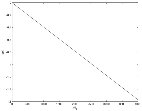
Figure 1: Computer simulated result of the difference between the approximate total phase and the exact total phase, where $\omega=0.01$, $\omega_{0}=10$,$\theta=\pi/6$.

Thus we have shown the total phase given by the traditional adiabatic theorem may have a remarkable error if the running time is very long. As a result, we must be careful if we combine the linearity of quantum mechanics and adiabatic approximation. Concretely, we can use the previous example to illustrate this point. Suppose the initial state of the system is

$$|\psi(0)\rangle=\frac{1}{\sqrt{2}}|E_{1}(0)\rangle+\frac{1}{\sqrt{2}}|E_{2}(0)\rangle.$$ (23)

Note that no matter which eigenstate the initial state is, the traditional adiabatic conditions are the same, because

$$|\langle E_{1}|\dot{E_{2}}\rangle|=|\langle E_{2}|\dot{E_{1}}\rangle|.$$ (24)

If the linearity of adiabatic approximation is valid, and if the common adiabatic condition

$$|\langle E_{1}|\dot{E_{2}}\rangle|\ll|E_{1}-E_{2}|.$$ (25)

is satisfied, it can be checked that the final state of the system will be

$$|\psi(\tau)\rangle\approx\frac{1}{\sqrt{2}}e^{-\alpha}|E_{1}(\tau)\rangle+\frac{1}{\sqrt{2}}e^{\alpha}|E_{2}(\tau)\rangle,$$ (26)

where, $\alpha=i\int E_{1}+\int\langle E_{1}|\dot{E_{1}}\rangle.$

However, based on Fig. 1, we know that there must be some $\tau$ such that the exact state of the system

$$|\psi^{\prime}(\tau)\rangle\approx\frac{1}{\sqrt{2}}e^{-\alpha-\frac{\pi}{2}i}|E_{1}(\tau)\rangle+\frac{1}{\sqrt{2}}e^{\alpha+\frac{\pi}{2}i}|E_{2}(\tau)\rangle.$$ (27)

Note that $\langle\psi(\tau)|\psi^{\prime}(\tau)\rangle\approx 0$. That is to say, the final state indicated by the linearity of adiabatic approximation is far from the exact final state. Thus, in this case the linearity of adiabatic approximation fails.

We have mentioned that the traditional adiabatic theorem has been criticized recently. Thus it is necessary to turn back to its proof and find out what is the problem. We will scrutinize the proof with the previous example in mind.

According to the proof, if the traditional adiabatic conditions are fulfilled the integral of the rhs of Eq.(8) will be small no matter how long the running time $\tau$ is. However, the example above tell us that this is not true. When gap between these two total phase is remarkable, this integral cannot be neglected. Thus there must be something wrong with the proof. Now we still use the previous example to find out the mistake. We think of the mistake as the root of the problem of the traditional adiabatic theorem.

Comparing Eq.(7) and Eq.(20), we have

$$\psi_{2}(t)=i\frac{\omega\sin{\theta}}{\bar{\omega}}\sin{\frac{\bar{\omega}t}{2}}e^{-i\frac{\omega_{0}t}{2}}e^{-i\frac{\omega\cos{\theta}}{2}t}.$$ (28)

At this time, the rhs of Eq.(8) is ($n=1$)

$$e^{i\int(E_{1}-E_{2})}\psi_{2}\langle e_{1}|\dot{e_{2}}\rangle=-\frac{(\omega\sin{\theta})^{2}}{\bar{\omega}}\sin{\frac{\bar{\omega}t}{2}}e^{i\frac{\omega_{0}+\omega\cos{\theta}}{2}t}.$$ (29)

The proof for the traditional adiabatic theorem at the beginning of this letter tells us that if the adiabatic condition

$$\frac{1}{2}\omega\sin{\theta}=|\langle e_{1}|\dot{e_{2}}\rangle|\ll|E_{1}-E_{2}|=\omega_{0}$$ (30)

is satisfied, the integral of the rhs of Eq.(29) can be negligible. Now we show that this is not true. In fact,

$$\begin{aligned} Im(\int_{0}^{\tau}\sin{\frac{\bar{\omega}t}{2}}e^{i\frac{\omega^{*}}{2}t}dt)=&\int_{0}^{\tau}\sin{\frac{\bar{\omega}t}{2}}\sin{\frac{\omega^{*}}{2}t}dt\\ =&\frac{1}{2}\int_{0}^{\tau}\cos{\frac{\bar{\omega}-\omega^{*}}{2}t}dt\\ -&\frac{1}{2}\int_{0}^{\tau}\cos{\frac{\bar{\omega}+\omega^{*}}{2}t}dt\\ =&\frac{1}{\bar{\omega}-\omega^{*}}\sin{\frac{\bar{\omega}-\omega^{*}}{2}\tau}\\ -&\frac{1}{\bar{\omega}+\omega^{*}}\sin{\frac{\bar{\omega}+\omega^{*}}{2}\tau},\end{aligned}$$

where $\omega^{*}=\omega_{0}+\omega\cos{\theta}$. Suppose $\omega_{0}\gg\omega\sin{\theta}$, it can be checked that

$$Im(\int_{0}^{\tau}e^{i\int(E_{1}-E_{2})}\psi_{2}\langle e_{1}|\dot{e_{2}}\rangle dt)\approx-2\sin{\frac{\bar{\omega}-\omega^{*}}{2}\tau}.$$ (31)

At the same time,

$$Re(\int_{0}^{\tau}e^{i\int(E_{1}-E_{2})}\psi_{2}\langle e_{1}|\dot{e_{2}}\rangle dt)\approx 2(\cos{\frac{\bar{\omega}-\omega^{*}}{2}\tau}-1).$$ (32)

It is obvious that $\sin{\frac{\bar{\omega}-\omega^{*}}{2}\tau}$ may be far from $0$ when $\tau$ is big. So the integral of the rhs of Eq.(29) cannot be negligible for all $\tau$. Thus a mistake in the proof for the traditional adiabatic theorem is found. When the traditional adiabatic conditions are satisfied, though the phase factor in Eq.(3) or Eq.(8) provides a rapid oscillation, the coefficients $\psi_{i}$ may do the same thing. This makes the integral that has been ignored not neglectable. This is the reason why the traditional adiabatic conditions are not sufficient to guarantee the validity of adiabatic approximation.

After the inconsistency was found, several attempts have been made to repair the traditional adiabatic conditions, for example Ref.YZZG05 and Ref.DMN05 . If we reexamine these new conditions, we will find that there are similar problems with the proofs for them. According to these two papers, in Eq.(8) we should consider not only the absolute value of $\langle e_{n}|\dot{e_{m}}\rangle$ but also its phase. Then when we integrate the rhs of Eq.(8) the integrand has a new phase factor. For the example we have considered Eq.(8) will be

$$i\dot{\psi_{1}}=-i\frac{1}{2}\omega\sin{\theta}\cdot\psi_{2}\cdot e^{i(\omega_{0}+\omega\cos{\theta})t}.$$ (33)

Now the modified adiabatic condition is

$$\omega_{0}+\omega\cos{\theta}\gg\omega\sin{\theta}.$$ (34)

However, we can see that in these two proofs the effects of $\psi_{n}$’s were not considered. In fact, as we have pointed out, $\psi_{n}$’s result in the consequence that the integral we have ignored cannot be neglected even if the modified adiabatic conditions are fulfilled.

Before concluding, we should emphasize that we cannot say quantum adiabatic theorem is invalid, though the traditional adiabatic conditions are insufficient. For an example of rigorous and sufficient but a litter complicated adiabatic conditions, we can see Ref.AR04 . This result states that in an adiabatic evolution if the path along which the Hamiltonian of the system varies is fixed (when the running time changes, the path does not), the adiabatic approximation will be valid as long as the evolution is slow enough. Thus this result guarantees the validity of quantum adiabatic computation FGGS00 .

Another point that should be stressed is that in the above example the running time $\tau$ that makes the adiabatic traditional proof fail is very long (See FIG. 1). When $\tau$ is not very long, the negligence in the proof is not fatal, and the adiabatic approximation is very good. Furthermore, perhaps in many cases, the phases of the $\psi_{n}$’s that we ignore is trivial (change slowly), then the adiabatic conditions are sufficient. As a consequence, the traditional adiabatic conditions are free of problems most of the time, but not always.

In conclusion, we have shown that in a quantum adiabatic evolution the approximate total phase of the final state proposed by Berry may differ evidently from the corresponding exact total phase when the running time is long enough. Because of this difference, we have to be very careful if we use both the linearity and quantum adiabatic approximation, especially when the running time of the adiabatic evolution is very long.

On the other hand, based on this difference, we have reexamined the traditional proof of the quantum adiabatic theorem. We show that there is an evident problem in the proof. We think this problem is the origin of the troubles the the traditional adiabatic theorem has met. This problem also exists in the proofs for some modifications of the traditional adiabatic conditions. In fact, these proofs all are based on the fact the integrals of rapid oscillations vanish. It seems that our discussion demonstrates that this is not a good way to lead to rigorous adiabatic conditions. Because we have known that $\psi_{n}$’s may have a considerable contribution to the integral. However, without solving the Schrödinger equation we cannot know anything about $\psi_{n}$’s.

We acknowledge D. M. Tong and Peter Marzlin for valuable comments and suggestions. We also thank C. P. Sun and the colleagues in the Quantum Computation and Information Research Group for helpful discussions. This work was partly supported by the National Nature Science Foundation of China (Grant Nos. 60503001, 60321002, and 60305005).

References

- (1) M. Born and V. Fock, Zeit.f.Physik 51, 165(1928).
- (2) L. I. Schiff, Quantum Mechanics (McGraw-Hill, Singapore, 1955).
- (3) M. V. Berry, Proc. R. Soc. London A 392, 45(1984).
- (4) Y. Aharonov and J. Anandan, Phys. Rev. Lett 58, 1593(1987).
- (5) J. Samuel and R. Bhandari, Phys. Rev. Lett 60, 2339(1988).
- (6) A. Uhlmann, Rep. Math. Phys 24, 229(1986).
- (7) E. Sjöqvist et al, Phys. Rev. Lett 85, 2845(2000).
- (8) P. Zanardi and M. Rasetti, Phys. Lett. A 264, 94(1999).
- (9) J. A. Jones, V. Vedral, A. Ekert and G. Castagnoli, Nature (London) 403, 869(2000).
- (10) E. Farhi, J. Goldstone, S. Gutmann, M. Sipser; e-print quant-ph/0001106.
- (11) K. -P. Marzlin and B. C. Sanders, Phys. Rev. Lett 93, 160408(2004).
- (12) D. M. Tong, K. Singh, L. C. Kwek and C. H. Oh, Phys. Rev. Lett 95, 110407(2005).
- (13) D. M. Tong, K. Singh, L. C. Kweh, X. J. Fan and C. H. Oh, Phys. Lett. A 339, 288(2005).
- (14) M. Y. Ye, X. F. Zhou, Y. S. Zhang and G. C. Guo, e-print quant-ph/0510131.
- (15) S. Duki, H. Mathur and O. Narayan, e-print quant-ph/0510131.
- (16) D. Comparat, e-print quant-ph/0607118.
- (17) A. Ambainis and O. Regev, e-print quant-ph/0411152.