Engineering correlation and entanglement dynamics in spin systems

Abstract

We show that the correlation and entanglement dynamics of spin systems can be understood in terms of propagation of spin waves. This gives a simple, physical explanation of the behaviour seen in a number of recent works, in which a localised, low-energy excitation is created and allowed to evolve. But it also extends to the scenario of translationally invariant systems in states far from equilibrium, which require less local control to prepare. Spin-wave evolution is completely determined by the system’s dispersion relation, and the latter typically depends on a small number of external, physical parameters. Therefore, this new insight into correlation dynamics opens up the possibility not only of predicting but also of controlling the propagation velocity and dispersion rate, by manipulating these parameters. We demonstrate this analytically in a simple, example system.

Correlations play a predominant role in the study of spin systems. On the one hand, they characterize different phases of matter, and thus can help reveal the mechanisms underlying phase transitions. On the other, they are directly related to the entanglement between different spins, which can be exploited by applications in the field of quantum information processing. Whereas so far, much of the work on correlations has focused on the static properties of equilibrium systems, an increasing interest in the corresponding dynamical properties has developed over the last few years. The reason is two fold. Firstly, new experimental setups, such as atoms in optical lattices, have reached an unprecedented level of control, allowing physical parameters to be changed during the experiments. Thus theoretical descriptions of the time-dependent properties of such systems have become important. Secondly, it has been recognized that the way entanglement is created and how it propagates are important fundamental questions in quantum information theory. In particular, the answers may influence the design of quantum repeaters and networks, whose goal is to establish as much entanglement as possible between different nodes in the shortest possible time.

The time evolution of correlation functions in spin systems has been studied recently in various scenarios, mainly from a condensed matter physics perspective. In Refs. Iglói and Rieger (2000); Amico et al. (2004), two-point correlations were studied numerically, whereas in Ref. Calabrese and Cardy (2006) their evolution in a critical model was studied analytically using conformal field theoretic methods. In all cases, correlations were seen to propagate at a finite speed. In Ref. Bravyi et al. (2006), a proof was given that correlations necessarily propagate at a finite speed. On the other hand, information and entanglement propagation in spin systems has mostly been studied from a quantum information perspective Osborne and Linden (2004); Bose (2003); Christandl et al. (2004); Cubitt et al. (2005).

In contrast with previous work, we will consider to what extent it is possible to control the propagation speed and dispersion of the correlations in a translationally invariant system, by tuning only simple, global, physical parameters. This may be relvant for the optimal creation of entanglement in spin systems, as well as contributing to a better understanding of how correlations are created in dynamical processes, something which can be tested experimentally in present setups. We will show that, even with this severely limited control over the system, the correlation speed can be engineered whilst simultaneously keeping dispersion to a minimum, so that correlations can be concentrated between particular spins. Indeed, by manipulating system parameters during the evolution, the speed can be adjusted at will, even to the extent of reducing it to zero, allowing correlations to be frozen at a desired location.

It is instructive to first consider the entanglement and correlation propagation described in the references given above from a new perspective. In many of those works, correlation propagation can be understood as follows. The spin system is initially prepared in its ground state. A localised, low-energy excitation is then created (e.g. by flipping one spin), and allowed to evolve. Since the low-energy excitations take the form of spin waves, the correlation and entanglement dynamics can be understood as nothing other than propagation of spin waves. This is completely determined by the dispersion relation (given by the system’s spectrum). The form of the dispersion relation will typically depend on external, physical parameters of the system (e.g. the strength of an external magnetic field). Thus already in these setups, we can manipulate the external parameters to control the dispersion relation, and hence control the propagation of correlations. For example, changing the gradient of the dispersion relation will change the propagation speed.

However, the ground state will typically be highly-correlated and difficult to prepare, and with the level of local control required to create the local excitation and break the translational symmetry, more sophisticated quantum-repeater setups are possible. Also, it is not clear that the correlations will remain localised; they are likely to disperse rapidly as they propagate.

Therefore, we will extend the idea to systems prepared in translationally invariant, easily created, uncorrelated initial states. For example, the fully polarised state with all spins aligned can be prepared by applying a large, external magnetic field. As the initial state will be far from the ground state, it will contain many excitations. The correlation dynamics is then the result of the propagation and interference of a large number of spin waves at many different frequencies. Nonetheless, we will show analytically that, at least for some simple models, the system can be engineered so that correlations propagate in well-defined, localised wave packets, with little dispersion. The external parameters can then be used to control the propagation of these correlation packets.

In the following, we will consider a specific model which, despite its simplicity, is sufficiently rich to display most of the features we are interested in. The model is simple enough to envisage implementing it experimentally, for instance using atoms in optical lattices or trapped ions. The XY–model for a chain of spin–$\frac{1}{2}$ particles is described by the Hamiltonian $H_{XY}=-\tfrac{1}{4}\sum_{l}((1+\gamma)\sigma^{x}_{l}\sigma_{l+1}+(1-\gamma)\sigma^{y}_{l}\sigma^{y}_{l+1}+2\lambda\sigma^{z}_{l})$, where the $\sigma$’s are the usual Pauli operators and the sum is over spin indices. The parameter $\lambda$ can be interpreted as the strength of a global, external magnetic field, whereas $\gamma$ controls the anisotropy of the interactions.

This Hamiltonian can be brought into diagonal form by the well-known procedure Sachdev (2001) of applying Jordan-Wigner, Fourier and Bogoliubov transformations, giving $H_{XY}=-\tfrac{i}{4}\sum_{k}\varepsilon_{k}(\gamma^{x}_{k}\gamma^{p}_{k}-\gamma^{p}_{k}\gamma^{x}_{k})$ with spectrum $\varepsilon_{k}=((\cos(2\pi k/N)-\lambda)^{2}+\gamma^{2}\sin^{2}(2\pi k/N))^{1/2}$. The $\gamma^{x,p}_{k}$ are Majorana operators, related to the more usual Jordan-Wigner fermionic annihilation operator $\gamma_{k}$ by $\gamma^{x}_{k}=\gamma_{k}^{\dagger}+\gamma_{k}$ and $\gamma^{p}_{k}=(\gamma_{k}^{\dagger}-\gamma_{k})/i$, and obey canonical anti-commutation relations $\left\{\gamma^{a}_{k},\gamma^{b}_{l}\right\}=2\delta_{k,l}\delta_{a,b}$.

Ultimately, we are interested in “connected” spin–spin correlation functions, for example the ZZ correlation function $C_{ZZ}(n,m)=\mathinner{\langle\sigma^{z}_{n}\sigma^{z}_{m}\rangle}-\mathinner{\langle\sigma^{z}_{n}\rangle}\mathinner{\langle\sigma^{z}_{m}\rangle}$, in which the “classical” part of the correlation is subtracted. These are related to the localisable entanglement $L(n,m)$ (the maximum average entanglement between two spins $n$ and $m$ that can be extracted by local measurements on all the others Verstraete et al. (2004)): the natural figure of merit for quantum repeaters. In particular, for spin–$\tfrac{1}{2}$ systems, $L(n,m)\geq C(n,m)$ for any connected spin–spin correlation function $C$ Popp et al. (2005). However, we will start by considering the simpler, albeit less well-motivated, string correlation functions such as $S_{XX}(i,j)=\mathinner{\langle\sigma^{x}_{i}(\prod_{i<k<j}\sigma^{z}_{k})\sigma^{x}_{j}\rangle}$ (important for revealing “hidden order” in certain models Affleck et al. (1988)). Their behaviour will give insight into the more important spin–spin correlations, and we will use similar techniques to calculate both.

Assume the spin chain is initially in some completely separable, uncorrelated state, such as the state with all spins down. The interactions are then switched on and, as this initial state is not an eigenstate of the Hamiltonian (unless $\lambda\to\infty$), the state evolves in time. The initial state is the vacuum of the Majorana operators $x_{l}\,(p_{l})=\prod_{j}\sigma^{z}_{j}\sigma^{x(y)}_{l}$ obtained after applying just the Jordan-Wigner transformation, and is completely determined by its two-point correlation functions. In other words, the vacuum is a fermionic Gaussian state, and can be represented by its covariance matrix $\Gamma_{m,n}=\tfrac{1}{2}\left<\left[r_{m},r_{n}\right]\right>$ where $r_{2l-1}=x_{l}$ and $r_{2l}=p_{l}$.

From the Heisenberg evolution equations, it is simple to show that any evolution governed by a quadratic Hamiltonian corresponds to an orthogonal transformation of the covariance matrix. It is also clear that, as the Fourier and Bogoliubov transformations are canonical (anti-commutation-relation-preserving) transformations of the Majorana operators, they similarly leave Gaussian states Gaussian, and they too can be expressed as orthogonal transformations. Thus the time-evolved state of the system is given by a series of orthogonal transformations of the fermionic vacuum:

$$\Gamma(t)=\mathcal{O}\Gamma_{\mathrm{vac}}\mathcal{O}^{T},\quad\mathcal{O}=O_{\mathrm{FT}}^{T}\,O_{\mathrm{Bog}}^{T}\,O(t).$$ (1)

This is a block-Toeplitz matrix, composed of $2\times 2$ blocks $G_{x}$ at distance $x$ from the main diagonal. In the thermodynamic limit $N\to\infty$ with $\frac{2\pi k}{N}\to\phi$ and $\varepsilon_{k}\to\varepsilon(\phi)\equiv\varepsilon$,

$$G_{x}=\int_{-\pi}^{\pi}\mathrm{d}\phi\begin{pmatrix}g_{0}&g_{1}\\ g_{-1}&g_{0}\end{pmatrix},\quad g_{0}=iS\sin(\phi x)\sin\bigl{(}2\varepsilon t\bigr{)}$$

$$\begin{split}g_{\pm 1}=2CS\sin(\phi x)&\sin^{2}\bigl{(}\varepsilon t\bigr{)}\pm\cos(\phi x)\Bigl{(}C^{2}+S^{2}\cos\bigl{(}2\varepsilon t\bigr{)}\Bigr{)}\end{split}$$

where $C=(\cos(\phi)-\lambda)/\varepsilon(\phi)$, $S=\gamma\sin(\phi)/\varepsilon(\phi)$, and $x=m-n$. We can now calculate certain string correlations, which are given directly by elements of the covariance matrix. For example, $\bigl{\langle}\sigma^{x}_{n}(\prod_{n<i<m}\sigma^{z}_{i})\sigma^{y}_{m}\bigr{\rangle}=\tfrac{1}{i}\Gamma_{2n-1,2m-1}=\sum_{s=\pm 1}s\int_{-\pi}^{\pi}\mathrm{d}\phi S\cos(\phi x+2s\varepsilon t)/2$.

Although the evolution of the string correlations is produced by the collective dynamics of a large number of excitations, this expression has a simple, physical interpretation: it is the equation for two wave packets with envelope $S/2$ propagating in opposite directions along the chain, according to a dispersion relation given by the system’s spectrum $\varepsilon(\phi)$. This wave-packet interpretation allows us to make quantitative predictions as to how the dynamics will be affected if the system parameters $\gamma$ and $\lambda$ are modified. Specifically, modifying the parameters will change the dispersion relation, changing the group velocity of the correlation packets, as well as the rate at which they disperse. (The wave-packet envelopes also depend on the system parameters, so the relevant region of the dispersion relation may also change.) Thus by varying only global physical parameters, we can control the speed at which correlations propagate.

Does this hold true for the more interesting spin–spin correlations? We will show analytically that they have a similar wave-packet description, although in terms of multiple packets propagating simultaneously. This will allow us to predict the behaviour of the spin–spin correlation dynamics for different values of the system parameters. In particular, we will show that the correlations can be made to propagate in well-defined packets whose speed can be engineered by tuning the system parameters. Moreover, the propagation speed can be controlled as the system is evolving, so we can speed up or slow down the packets, even to the extent of reducing the speed to zero. We confirm our predictions by numerically evaluating the analytic expressions.

Let us now calculate the spin–spin connected correlation function using the covariance matrix derived above. We have $\sigma^{z}_{n}=x_{n}p_{n}$, so the ZZ connected correlation function is given by $C_{ZZ}(x)=\mathinner{\langle x_{n}p_{m}\rangle}\mathinner{\langle p_{n}x_{m}\rangle}-\mathinner{\langle x_{n}x_{m}\rangle}\mathinner{\langle p_{n}p_{m}\rangle}$, where we have used Wick’s theorem to expand the expectation value of the product of four Majorana operators into a sum of expectation values of pairs Wick (1950); Cubitt and Cirac . The latter are given by covariance matrix elements, resulting in the following analytic expression for the correlation function:

$$\begin{split}&C_{zz}(x,t)^{2}=\\ &\biggl{(}\int_{-\pi}^{\pi}\mathrm{d}\phi\,\frac{S}{2}\sum_{s=\pm 1}\bigl{(}s\cos(\phi x-2s\varepsilon t)\bigr{)}\biggr{)}^{2}\\ &+\biggl{(}\int_{-\pi}^{\pi}\mathrm{d}\phi\,CS\bigl{(}\sin(\phi x)-\frac{1}{2}\sum_{s=\pm 1}\sin(\phi x+2s\varepsilon t)\bigr{)}\biggr{)}^{2}\\ &-\biggl{(}\int_{-\pi}^{\pi}\mathrm{d}\phi\,\bigl{(}C^{2}\cos(\phi x)+\frac{S^{2}}{2}\sum_{s=\pm 1}\cos(\phi x+2s\varepsilon t)\bigr{)}\biggr{)}^{2}.\end{split}$$ (2)

Although more complicated than the string correlations, this expression also describes wave packets evolving according to the same dispersion relation $\varepsilon(\phi)$, albeit multiple packets with different envelopes propagating and interfering simultaneously (three in each direction). In many parameter regimes, broad (in frequency-space) wave packets and a highly non-linear dispersion relation will cause the correlations to rapidly disperse and disappear. However, we can find regimes in which the wave packets are located in nearly linear regions of the dispersion relation, and maintain their shape as they propagate. For example, at $\gamma=1.1$ and $\lambda=2$, all three wave packets of Eq. (2) are nearly identical, and reside in an almost-linear region of the dispersion relation with gradient roughly equal to 2, as shown in Fig. 1 (inset). The spin–spin correlation dynamics will therefore involve well-defined correlation packets propagating at a speed $\mathrm{d}x/\mathrm{d}t=2$, dispersing only slowly as they propagate. Fig. 1 shows the result of numerically evaluating Eq. (2), which clearly confirms the predictions.

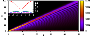
Figure 1: For $\gamma=1.1$, $\lambda=2$, all the wave-packet envelopes from Eq. (2) (non-red curves, inset) are similar in form, centred around a nearly linear region of the dispersion relation with gradient $\approx 2$ (red curve, inset). Thus the correlations $C_{zz}(x,t)$ (indicated by the shading, main plot) propagate in well-defined packets at a speed given by the gradient.

We can engineer a different correlation speed by changing the parameters. For instance, for $\gamma=10$ and $\lambda=0.9$ we predict a higher propagation speed $\mathrm{d}x/\mathrm{d}t\approx 18$, although at the expense of increased dispersion. The numerical results of Fig. 2 show precisely this behaviour.

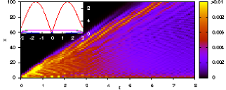
Figure 2: For $\gamma=10$, $\lambda=0.9$, the wave-packet envelopes are spread over the entire frequency range (non-red curves, inset). However, the dispersion relation (red curve, inset) is almost linear for wavenumbers not too near $\pi$, with gradients $\pm 18$. As the envelopes are symmetric about $\pi$, most of the correlations $C_{zz}(x,t)$ (shading, main plot) still propagate at a well-defined speed $\approx 18$, faster than in Fig. 1 (note scale), though as expected they also show more dispersion.

An even more interesting possibility is controlling the correlation packets as they propagate. If the system parameters are changed continuously in time, the XY-Hamiltonian becomes time-dependent, and the orthogonal evolution operator $O(t)$ in Eq. (1) is given by a time-ordered exponential $O(t)=T[e^{\int_{0}^{t}\mathrm{d}t^{\prime}A(t^{\prime})}]\equiv\lim_{h\to 0}\prod_{n=1}^{\lfloor t/h\rfloor}e^{A(nh)}$. ($A$ is a time-dependent, anti-symmetric matrix determined by the Hamiltonian.) In general, the time-ordering is essential. But if the system parameters change slowly in time, dropping it will give a good approximation to the evolution operator. The state at time $t$ is then just given by evolution under the time-average (up to $t$) of the Hamiltonian. If we remain in a parameter regime for which the relevant region of the dispersion relation is nearly linear, adjusting the parameters changes the gradient without significantly affecting its curvature or the form of the wave packets. Thus, to good approximation, slowly adjusting the parameters should control the speed of the wave packets as they propagate, allowing us to speed them up and slow them down. Numerically evaluating the time-ordered exponential shows this is indeed possible (Fig. 3).

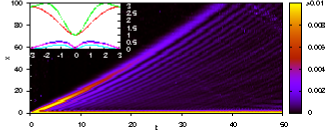
Figure 3: Starting from $\gamma=1.1$, $\lambda=2$ as in Fig. 1, $\gamma$ and $\lambda$ are smoothly changed to move from the red to the green dispersion relation (inset), increasing the correlation speed.

Clearly it would be useful to be able to stop the correlations once they reach a desired location. One way would be to simply switch off the interactions. But strictly speaking this would require more control than is provided by the two parameters defined in the Hamiltonian (there is no value of $\gamma$ for which all interaction terms vanish), and may be difficult in physical implementations. If the spin model were realised in a solid-state system, for example, switching off the interactions would likely involve fabricating an entirely new system. In any case, we will show that switching off the interactions is not necessary in order to freeze correlations at a specific location.

Instead of changing the parameters continuously, we now consider changing them abruptly. The time-evolved covariance matrix in this scenario can be calculated analytically by the same methods as used above. Suppose the initial system parameters $\gamma_{0}$ and $\lambda_{0}$ are suddenly changed to $\gamma_{1}$ and $\lambda_{1}$ at time $t_{1}$. The spin–spin correlations will initially evolve according to Eq. (2), as before. After time $t_{1}$, the evolution becomes more complicated. The analogue of Eq. (2) separates into a sum of wave packets evolving in four different ways: those that initially evolve according to $\varepsilon_{0}$ and subsequently (after $t_{1}$) evolve according to $\varepsilon_{1}$, those that subsequently evolve according to $-\varepsilon_{1}$, those that only start evolving at $t_{1}$, and those that that undergo no further evolution after $t_{1}$ (Fig. 4). For $t>t_{1}$, the terms whose evolution is “frozen” at time $t_{1}$ are given by

$$C_{z}^{t_{1}}(x,t)^{2}=$$

$$\left(\frac{1}{2}\int_{\mathchoice{\hbox to0.0pt{$\displaystyle{-\pi}$\hss}}{\hbox to0.0pt{$\textstyle{-\pi}$\hss}}{\hbox to0.0pt{$\scriptstyle{-\pi}$\hss}}{\hbox to0.0pt{$\scriptscriptstyle{-\pi}$\hss}}}^{\mathchoice{\hbox to0.0pt{$\displaystyle{\pi}$\hss}}{\hbox to0.0pt{$\textstyle{\pi}$\hss}}{\hbox to0.0pt{$\scriptstyle{\pi}$\hss}}{\hbox to0.0pt{$\scriptscriptstyle{\pi}$\hss}}}\mathrm{d}\phi S_{0}S_{1}(C_{0}S_{1}-C_{1}S_{0})\sum_{s=\pm 1}\sin(\phi x+2st_{1}\varepsilon_{0})\right)^{2}$$

$$-\left(\frac{1}{2}\int_{\mathchoice{\hbox to0.0pt{$\displaystyle{-\pi}$\hss}}{\hbox to0.0pt{$\textstyle{-\pi}$\hss}}{\hbox to0.0pt{$\scriptstyle{-\pi}$\hss}}{\hbox to0.0pt{$\scriptscriptstyle{-\pi}$\hss}}}^{\mathchoice{\hbox to0.0pt{$\displaystyle{\pi}$\hss}}{\hbox to0.0pt{$\textstyle{\pi}$\hss}}{\hbox to0.0pt{$\scriptstyle{\pi}$\hss}}{\hbox to0.0pt{$\scriptscriptstyle{\pi}$\hss}}}\mathrm{d}\phi S_{0}C_{1}(C_{0}S_{1}-C_{1}S_{0})\sum_{s=\pm 1}\cos(\phi x+2st_{1}\varepsilon_{0})\right)^{\mathchoice{\hbox to0.0pt{$\displaystyle{2}$\hss}}{\hbox to0.0pt{$\textstyle{2}$\hss}}{\hbox to0.0pt{$\scriptstyle{2}$\hss}}{\hbox to0.0pt{$\scriptscriptstyle{2}$\hss}}}.$$

Since $t$ does not appear on the right hand side, this expression clearly describes wave packets that propagate until time $t_{1}$ and then stop. Using these, we can move correlations to the desired location, then “quench” the system by abruptly changing the parameters, freezing the correlations at that location, as shown in Fig. 4.

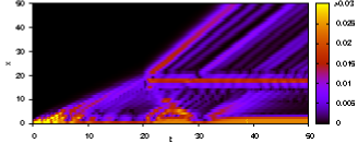
Figure 4: The system is initially allowed to evolve with $\gamma_{0}=0.9$ $\lambda_{0}=0.5$, then “quenched” at time $t_{1}=20$ to $\gamma_{1}=0.1$, $\lambda_{1}=10$. Some of the correlations are frozen at the separation ($x\approx 20$) they reached at $t_{1}$. Others propagate according to the new dispersion relation, or are “reflected”.

We have shown that entanglement and correlation propagation in many spin-model setups can be understood in terms of propagation of spin waves, and have introduced the idea of controlling the dynamics via their dispersion relation, by manipulating external parameters of the system. Although this is in principle possible for almost any spin system, preparing a single-excitation initial state would require control over individual spins. Therefore, we have analysed in detail the more complex case of systems prepared in uncorrelated, translationally invariant initial states, which typically contain many excitations. We have shown for an example model that the dynamics can be described by a small number of correlation wave packets, and that the control afforded by a few external, physical parameters is sufficient to allow detailed control over the propagation of correlations.

References

- Iglói and Rieger (2000) F. Iglói and H. Rieger, Phys. Rev. Lett. 85, 3233 (2000).
- Amico et al. (2004) L. Amico et al., Phys. Rev. A. 69, 022304 (2004).
- Calabrese and Cardy (2006) P. Calabrese and J. Cardy, Phys. Rev. Lett. 96, 136801 (2006).
- Bravyi et al. (2006) S. Bravyi, M. B. Hastings, and F. Verstraete, quant-ph/0603121 (2006).
- Osborne and Linden (2004) T. J. Osborne and N. Linden, Phys. Rev. A. 69, 052315 (2004).
- Bose (2003) S. Bose, Phys. Rev. Lett. 91, 207901 (2003).
- Christandl et al. (2004) M. Christandl, N. Datta, A. Ekert, and A. J. Landahl, Phys. Rev. Lett. 92, 187902 (2004).
- Cubitt et al. (2005) T. S. Cubitt, F. Verstraete, and J. I. Cirac, Phys. Rev. A. 71, 052308 (2005).
- Sachdev (2001) S. Sachdev, Quantum Phase Transitions (CUP, 2001).
- Verstraete et al. (2004) F. Verstraete, M. Popp, and J. I. Cirac, Phys. Rev. Lett. 92, 027901 (2004).
- Popp et al. (2005) M. Popp, F. Verstraete, M. A. Martin-Delgado, and J. I. Cirac, Phys. Rev. A. 71, 042306 (2005).
- Affleck et al. (1988) I. Affleck, T. Kennedy, E. H. Lieb, and H. Tasaki, Comm. Math. Phys. 115, 477 (1988).
- Wick (1950) G. C. Wick, Phys. Rev. 80, 268 (1950).
- (14) T. S. Cubitt and J. I. Cirac, in preparation.