Decoherence and the appearance of classicality

in physical phenomena

Daniel Bar

Department of Physics

Ph. D. Thesis

Submitted to the Senate of Bar-Illan University, Ramat-Gan, Israel

October 2002

Several parts of this thesis,

mainly the quantum ones, were

worked in consultation with

Professor L. P. Horwitz

Department of Physics         Bar-Ilan University

Acknowledgement

I wish to thank Professor L. P. Horwitz.

I wish, especially, to thank my brother Moshe without his help

not only this thesis but also all my academic studies would not

be possible.

Where Science has progressed the farthest, the mind has but regained from nature that which the mind has put into nature.

Arthur. S. Eddington

in

Space Time and Gravitation

BIBLIOGRAPHY . . . . . . . . . . . . . . . . . . . . . . . . . . . . . . . . . . . . . . . . .78

0.1 List of figures

Figure 3.1:         Schematic representation of the concentric circular billiard that

simulates the reversible reaction $A+B\leftrightarrow C+D$. ………………………………………….29

Figure 3.2:         The three curves represent the activities obtained when all the particles

are: (1) only in “state” 1. (2) only in “state” 2. (3) allowed to pass between

the two “states” after every 1100 reflections. …………………………………………………29

Figure 3.3:         The two curves represent the activities obtained when all the particles are:

(1) only in “state” 2. (2) allowed to pass from “state” 1 to 2 after each

reflection and from 2 to 1 after every 1100 reflections. …………………………………….32

Figure 3.4:        The two curves represent the activities obtained when all the particles are:

(1) only in “state” 1. (2) allowed to pass from “state” 2 to 1 after each

reflection and from 1 to 2 after every 1100 reflections. …………………………………….32

Figure 3.5:        This Figure show the activities obtained when the degree of "densing" is

changed slightly from reactioning after each single reflection

to doing that after every two reflections (compare with Figure 5.3) ……………………33

Figure 5.1:        Seven representative Feynman paths of states. The collective dense

measurement is done along the middle one. ………………………………………………….44

Figure 5.2:        A schematic representation of the physical situation after performing

the collective dense measurement shown in Figure 5.1. The emphasized

path is common to all the ensemble. ……………………………………………………………46

Figure 5.3:         A three-dimensional surface of the relative rate of the number of

observers as function of the number of possible results $K$ for each

experiment and the number $r$ of places occupied by preassigned

eigenvalues………………………………………………………………………………………………50

Figure 5.4:        The cylinder with the four pistons. ………………………………………………………………54

Figure 5.5:        A three-dimensional surface of the entropy per molecule $s$ as a function

of the fractions $\frac{n_{o}}{n}$ and $\frac{n_{i}}{n}$ of molecules that step out and into the

interval $(-x,x)$…………………………………………………………………………………………57

Figure 5.6:         The result of perfoming 1000 different experiments of lifting up the pistons

as a function of the number of observers $N$. …………………………………………………..59

Figure 5.7:        The same as Figure 15 except that the values of $(-x_{j},x_{j})$, $\frac{n_{o_{j}}}{n}$ and $\frac{n_{i_{j}}}{n}$

are chosen randomely…………………………………………………………………………………59

0.2 Abstract

It is accepted that among the ways through which a quantum phenomenon decoheres and becomes a classical one is what is termed in the literature the Zeno effect. This effect, named after the ancient Greek philosopher Zeno of Elea (born about 485 B.C), were used in 1977 to analytically predict that an initial quantum state may be preserved in time by merely repeating a large number of times, in a finite total time, the experiment of checking its state. Since then this effect has been experimentally validated and has become an established physical fact. It has been argued by Simonius that the Zeno effect must be related not only to quantum phenomena but also to many macroscopic and classical effects. Thus, since it operates in both quantum and classical regimes it must cause to a more generalized kind of decoherence than the restricted one that “classicalizes” a quantum phenomenon. We show that this generalized decoherence, obtained as a result of dense measurement, not only gives rise to new phenomena that are demonstrated through new responses of the densely interacted-upon system but also may physically establish them. For that matter we have found and established the analogous space Zeno effect which leads to the necessity of an ensemble of related observers (systems) for the remarked physical validation of new phenomena. As will be shown in Chapters 3-5 of this work the new phenomena (new responses of the system) that result from the space Zeno effect may be of an unexpected nature. We use quantum field theory in addition to the more conventional methods of analysis and also corroborate our analytical findings by numerical simulations.

Chapter 1 Introduction

1.1 Static and dynamic Zeno effects

We wish to discuss in this work, as its name implies, the detailed stages of the decoherence process, where by this term we mean also the mechanism that not only physically validates and establishes a new-encountered phenomenon [1] but also, as will be shown, may initially give rise to it [1]. We note that one generally finds in the literature (see, Giulini et al in [2] and references therein) this term as meaning the process that “classicalizes” a quantum phenomenon so that its former wavy character disappears [3]. In this work we also take this term more generally to mean the process that may first give rise to a new phenomenon, in a manner to be fully described in this work, and then physically establish it. The involved process includes the stages of first trying [4], especially through mathematical expressions, to explain this phenomenon and then of validating (or refuting) the suggested expression by experiments. The last stage, in which one tests the assumed mathematical relation to see if it conforms to the experimental findings, is the most important one since by this one may decide the status of the assumed theory to be either elevated to the physical level or to be refuted. We note that since the advent of quantum mechanics there is in the literature a long and continuous effort that tries to clarify and understand the problem of measurement (see, for example, [5, 6, 7, 8]).

We wish to describe by various examples the means through which a new phenomenon is first discerned as such and then decoheres to become an established physical fact. We do this by various methods that, although appear to be different at first sight, nevertheless, they all yield the same result that what may first initiate and then physically establish a new phenomenon (and the theory that explains it) is not only the experiment one performs in order to test it but the multiple repetitions of it (or of similar versions of it) in a finite total time [4, 9] as will be explained. Moreover, we show that the degree of validity depends upon the number of these repetitions, that is, the more large is this number in the total alloted time the more physically established the phenomenon and its proposed theory will be [4].

These repetitions are regarded by many authors [2, 10, 11, 12, 13] as an important factor in giving rise to the remarked restricted decoherence through which a quantum phenomenon becomes “classicalized”. This appearance of classicality in the quantum regime is termed the quantum Zeno effect [2, 10, 11, 12, 13, 14] and it denotes the mechanism by which the initial state of some quantum system is preserved in time by only repeating a large number of times, in a finite total time, the experiment of checking its state. The last result is termed the quantum static Zeno effect [12] to differentiate it from the quantum dynamic Zeno effect [12] which is not composed of repeating the same experiment but of performing a very large number of different experiments each of them reduces the system to different state so that it proceeds through a specific path of consecutive states. Thus, if the different experiments that reduce the system to this path are done in a dense manner this results in “realizing” this path, from the large number of possible different ones, as has been demonstrated theoretically [11, 12] and experimentally [10]. This “realization” is effected through the probability to proceed along the different possible paths of states which tends to unity for the one that dense measurements were performed along it and to zero for the others.

It has been argued [14] that the Zeno effect is not restricted only to quantum events but it may be found also in many macroscopic and classical phenomena. That is, even the classical phenomena are established as a result of the Zeno effect. In other words, this process may be the source that causes, through the remarked repetitions, the “realization” of many physical phenomena and not only to their “classicalization” from any former quantum stage they may be in. We show in the following that this effect may indeed establish the physical character (and not only the classical properties) of many phenomena.

We show that since these repetitions are an important factor in constituting the physical aspect of real phenomena then the reality of the latter do not depend only on their specific nature but also on this dense measurement. That is, we expect to find this Zeno effect demonstrated in many disciplines of physics, as well as other scientific regimes, as has been argued in [14]. This effect has indeed been experimentally found in diverse phenomena [10] including chemistry [13]. We have shown its possible existence in both quantum [1, 15, 16, 17, 18] and classical phenomena [19, 20, 21] and also in chemical reactions [22].

One may argue that all the real phenomena, physical, chemical, biological etc do not seem to obtain their reality from any repetitions at all, so how and in what manner these supposed iterations become effective in the remarked physical validation ?. That is, our physical laws and phenomena do not appear to result from any dense measurement as described here. The answer is that the relevant repetitions that may establish the physical character of the real phenomena are not the time repetitions one usually connects [2, 10, 11, 12, 13, 14] with the Zeno effect but a space version of it. That is, in order to appropriately discuss the process of physically establishing the new-encountered phenomena we have introduced a new kind of Zeno effect which we call space Zeno effect [4, 17, 18, 20, 23]. In the last effect, to be fully discussed in the following chapters, the remarked dense repetitions are done in space and not in time so that the relevant ensemble is of related observers (systems) in space and not of repeated experiments in time. This effect stands in the basis of the remarked physical validation of new phenomena as we later show in Chapters 3-5 when we discuss the effect of the large ensemble of related observers. That is, the repetitions effected in the physically establishing process are not the conventional ones of the time Zeno effect [2, 10, 11, 12, 14] that are performed serially in time but those that are done by a large ensemble of observers.

Moreover, the number of observers in the ensemble does no have to be large in order to accomplish this establishing process. This may be seen clearly from Section 4.3 (see also [17] which is partly shown in Appendix $C_{2}$) where we discuss the one-dimensional multibarrier potential of finite range which constitutes a quantum example of the space Zeno effect in which the barriers in the finite spatial axis represent a one-dimensional version of observers (systems). One may realize from Figures 2-5 in [17], which are shown also in Appendix $C_{2}$, that for both cases of $e>v$ and $e<v$ and for either a constant or a variable length of the finite section, along which the barriers are arrayed, it is possible to obtain a significant transmission of the passing wave even for a 30 potential barriers. This may be seen also for the analogous classical one-dimensional multitraps in a finite section as seen in the relevant papers [20, 21] (see these articles, and especially their graphs in Appendices $C_{4}$-$C_{5}$). This significant, and unexpected, transmission of the particles (either quantum or classical) through the barriers or traps constitutes the new response (phenomenon) that not only comes into being as a result of this multi-measuring process but also may be established by repeating these kinds of experiments. In summary, one does not have to take the limit of a very large number of systems (observers) for obtaining this new response and for physically establishing it.

1.2 Time and space Zeno effects

The remarked repetitions, of either the same experiment or along a large set of different ones, that characterize the static and dynamic Zeno effects respectively are performed in time. Thus, an important element of these repetitions is, as remarked, that they must be done in a finite total time $T$ so that both Zeno effects are obtained in the limit in which the number $N_{t}$ of repetitions in $T$ satisfies $N_{t}\to\infty$. It has been shown [4, 23, 24] that the same effect is obtained also when these experiments are performed on a large number of similar systems occupied in a finite region of space $R$ instead of repeating it a large number of times, in a finite total time $T$, on the same system. The corresponding space Zeno effect is obtained [4, 23, 24] in the limit when the number of systems $N_{r}$ ( observers) in $R$ satisfies $N_{r}\to\infty$. We note that what characterizes both kinds of the Zeno effect is the continuous and uninterrupted experimentation either in time or space so there is no time (in the total time) or region (in the total spatial volume) that the system is not interacted upon. Thus, this kind of uninterrupted experimentation in which the system is not left to itself causes it to behave differently, even unexpectedly as will be shown, especially, in Chapters 3-5. Moreover, as remarked, the dense measurement condition not only gives rise to this new behaviour of the system but may also physically establish it.

We must note that we do not regard each separate experiment as constituting an experiment on its own, only the whole array of all these similar experiments, all confined to be done in a finite region of space, is considered as an experiment. The conclusion obtained is that in such a limit, when the magnitude of each experimental set-up becomes very small whereas the total volume (in which all these experiments are performed) does not change, we get actually, as remarked, a field of such probes (see Section 1.4 of this work, Bixon in [13], and [26]). In such cases it is meaningless to discuss these fields in terms of the separate points as it is meaningless to treat the electromagnetic field pointwise. The same is true also for the time Zeno effect. That is, it is necessary to look upon the whole array of these elements of measurements, and from such a perspective the Zeno effect is obtained not only theoretically but also experimentally, as has been done for the time Zeno effect by Itano et al [10]. Kofman and Kurizki in [10] show the existence of this effect with regard to the excitation decay of the atom in open cavities and waveguides using a sequence of pulses on the nanosecond scale; see also Raisen in [10] for another way of showing experimentally the Zeno effect, this time in quantum tunnelling.

Thus, we may regard the whole process, composed of the large number of repetitions of the same experiment, as one inseparable process that should not be decomposed as we show in the following. This view is related to that adopted, for example, by Gell-Mann-Hartle-Griffiths [27, 28, 29] in their histories formalism (see Section 2.2 of this work). In this formalism only the complete history is regarded as a physical process and the separate parts of it are not considered to be reduced physical entities on their own. It has been shown in [1], by discussing in terms of Feynman paths [30, 31, 32] the three processes of the EPR paradox [33], the Wheeler’s delayed choice experiment [5], and the teleportation phenomenon [34], that the paradox in these processes arises only from discussing them before they are complete. For example, in the EPR process, we assume that one particle of the two involved must always have some definite direction for its spin even before we measure the spin of the second particle [33]; but the EPR experiment is complete only after the latter measurement is performed. Thus, the Zeno effect should be discussed on the basis of the entire ensemble of repetitions without considering the particular experiment that is repeated. This has been shown in [35] by using the geometric structure of the Fubini-Study metric defined on the projective Hilbert space of the quantum system. With the help of this projective geometry a quantum Zeno effect has been predicted for many types of systems even those described by nonlinear and nonunitary evolution equations, that is, even the linear Schroedinger equation is not a necessary condition.

1.3 Single and ensemble of observers

The differences between the time Zeno effect and its space analog constitute, as remarked, the important differences between the case when the remarked dense experiments are done by one observer or by a large number of them [4] (where in the last case no one has to repeat his specific experiment). That is, the time Zeno effect corresponds to the first case and its space analog to the second. In the first case one may establish his tested theories for himself but, as should be obvious, this will not be common to other unrelated observers. When, however, a large ensemble of observers is involved the relevant new phenomenon and its theory will be physically established, for all of them, without having each one repeating his experiment so long as they are related to each other in the sense that the results of any specific experiment done by any one of them are valid also for all the others. That is, although only one, from a large number of observers, does his specific experiment, nevertheless, the relationship among the ensemble members, to be discussed in details in Chapters 3-5 of this work, ensures that any other observer that repeat the same experiment under the same conditions obtains the same results. We show that the more large is the ensemble of related observers that perform the experiments the more physically established for all of them will be the new phenomenon and its theory [4].

1.4 Field realization of the Zeno effect

The physical validation of new phenomena due to densely experimenting with a large ensemble of systems that are confined in a finite region of space necessitates, as remarked in Section 1.2, to discuss these systems, especially in the limit of a large number of them, in terms of fields. That is, when the number of systems increases whereas the total volume does not change the magnitude of each system becomes very small and we get actually, as remarked, a field of them. The known physical fields, such as the electromagnetic field, can be regarded as such fields of probes as has been done by several authors. Bixon in [13] has shown that the stabilization of the localized Born-Oppenheimer states [37] is due to the surrounding medium composed from such a field of probes. In his article Bixon himself regards this stabilizing effect of the surrounding field as a manifestation of the Zeno effect, although he regards it as the conventional time Zeno effect and not its space analog. Davies [26] has likewise treated the electromagnetic field as a field of probes and show that the interaction with it causes the localized state to acquire lower energy than the extended one, thus stabilizing it. It seems, therefore, appropriate to use field formalism in order to discuss this effect. We exploit in the following both quantum [38, 39] and classical field [40, 41, 42] methods for demonstrating the possible existence of the Zeno effect in various different phenomena.

1.5 Numerical simulations as corresponding to Zeno processes

An important example in which the effect of the large ensemble of related systems (observers) is sharply pronounced is, as shown in [9, 51], that of computer numerical simulations. In this respect we point out the striking similarity of the remarked repetitions that lead to establishing and validating of real phenomena to the corresponding numerical repetitions of many computer simulations especially those concerned with finding numerical solutions of physical problems. For example, the numerical solution of any differential equation, including those that govern the evolution of physical systems, is obtained only after repeatedly updating the given differential equation. Moreover, the larger is the number of these iterations the larger will be the number of samples and the better is the resulting statistics. Thus, there is a strong correspondence between the remarked stages of physically establishing a new phenomenon to the mechanism of numerical simulation [9]. An important example of numerical simulations, discussed in [9, 51], is related to Internet webmastering [9, 51], where by this term we mean the stages of first writing the software sources of the websites (by HTML, Java or other script) then running these codes to show the relevant websites on the computer screen. We extensively discuss in [9, 51] the stages of these numerical simulations and especially those related to their code-writing and conclude from the obtained results about the corresponding processes of real phenomena (see especially [9]).

1.6 Scope of this work

This work is composed of five chapters, the first of which is the present introduction, that are connected by the unifying principle of the Zeno effect. Each chapter is constructed from several sections that may serve as preliminary introductions to the main calculations and results that have been published in articles (see list of publications at the end of this work). The relevant papers are shown completely or partly in special Appendices in this work. The common result demonstrated in the five chapters and their relevant articles in the Appendices is that the factor that causes a physical system to first responds in a different, even unexpected, manner and then physically establish this new response (new phenomenon) is, as remarked, the repetitions of experiments embodied in the time and, especially, in the space Zeno effect.

In Chapter 2 we discuss the time Zeno effect in the framework of quantum field theory. Section 2.1 discusses both kinds of the static and dynamic Zeno effects by using the quantum field examples analyzed in [25] (which is completely shown in Appendix $A_{1}$). We show by these examples that experimenting in an uninterrupted manner on the system results in a new response of it that occurs only because of this kind of experiment. Thus, all one have to do in order to reconstruct this new response of the system is to perform again dense measurement. In other words, this kind of experimentation not only gives rise to this new result but also physically establishes and validates it. We also show that the Zeno process is responsible for the occurence of additional effects that do not appear in the absence of the relevant repetitions [25]. Section 2.2 discusses the histories formalism [27, 28, 29] in conjunction with the Flesia-Piron quantum extension [43] of the Lax-Phillips theory [44]. We show, using the results of [45] which is shown in Appendix $A_{2}$, that the histories evolution is stationary if the corresponding elements of the sequence $(h_{t_{1}},h_{t_{2}},h_{t_{3}},\ldots)$, which denotes the relevant history in a Lax-Phillips sense [43, 44], are determined by the Schröedinger evolution between infinitesimally close neighbours in this sequence. That is, the stability of the real histories evolution corresponds to the dynamic Zeno effect [11, 12]. We also show that the static Zeno effect is obtained if all the elements of the former sequence are identical so that $h_{t_{k}}=h_{t_{0}}$ for all $k=1,2,3,\ldots$.

As remarked, the Zeno effect is not restricted only to quantum events but is effective also in the classical regime. This may be realized from [9] in which we apply the stochastic quantization (SQ) method of Parisi-Wu [42, 46] to the programming process that simulates physical phenomena. We use in [9] the path integral method [30, 31, 32] to show the effect of the remarked repetitive element. For this method the repetitions are effected through introducing into the actions $S$ of all the path integrals of the relevant ensemble the same expression that determines the involved process. In [51] we discuss the Internet websites without referring to any particular site. We use for that purpose a statistical machanics approach [47, 48, 49, 50] that allows us to consider large clusters of mutually linked sites [51]. We obtain similar results to those obtained from the SQ method, discussed in [9], and from the Feynman diagram summation [30, 31, 32] of Chapter 2. In all these methods one obtains, as will be shown, in the limit of a very large number of these repetitions, the known physical, or numerical, equilibrium situations.

In Chapter 3 we apply the Zeno effect to the general reversible classical chemical reaction $A_{1}+A_{2}+\ldots\leftrightarrow B_{1}+B_{2}+\ldots$. We show that in the limit of repeating this reaction a large number of times one remains with the initial constituent particles as if the reaction never happened. That is, one obtains the remarked static Zeno effect. We have also demonstrated in Section 3.3 the possible existence of the dynamic Zeno effect in classical chemical reactions. These results were also numerically demonstrated in Section 3.4 using the double circular billiard model [19, 22]. This numerical billiard model was first introduced in [19] to show the classical effects of dense measurement and in Section 3.4 we use this model for simulation of classical reactions. The paper [19] is completely shown in Appendix $B_{1}$.

In Chapter 4 we discuss the space Zeno effect in both its quantum and classical realizations. We do this with the help of the Appendices $C_{1}$, $C_{2}$, $C_{3}$ and $C_{4}$ which show the papers or the relevant parts of them that discuss this aspect of the Zeno effect. In Section 4.2 we show, using [23] which is partly shown in Appendix $C_{1}$, that the relevant expression for the space Zeno effect may be derived analytically [23] from that of the time Zeno effect by replacing, and doing the appropriate changes, the time variable by the space one. In Section 4.3 we discuss two systems that although appear similar at first sight they are very different fron each other since one is quantum and the other is classical. We show for both systems the existence of the space Zeno effect. The first one which is discussed in the papers [17] and [18], which are shown in Appendices $C_{2}$ and $C_{3}$ respectively (only Sections 1-2 of [17] is shown in $C_{2}$), is the quantum one-dimensional multibarrier potential of finite range and the second, discussed in [20, 21], is the classical one-dimensional array of imperfect traps (the papers [20], [21] are shown in the Appendices $C_{4}$ and $C_{5}$ respectively). we have demonstrated for the first quantum system also chaotic [17, 18] and phase transition [52] effects. The existence of the space Zeno effect for each system and for both cases of finite and infinite number of barriers or traps in the finite interval is demonstrated. That is, we show analytically and numerically, for both systems, the somewhat unexpected result [17, 18, 20, 21] that the larger is the number of barriers or traps the value of either the probability amplitude of the quantum wave after passing the barriers or the density of the classical diffusing particles after going through the traps tends to the initial value before traversing either system.

We have discussed, especially, these quantum and classical systems since they both exhibit the noted characteristics of the Zeno effect. That is, an uninterrupted experimentation, in a spatial sense as will be explained in Chapters 4-5, on either one causes them to behave differently and unexpectedly compared to their known behaviours in the absence of these spatial dense measurement. That is, their known and expected physical behaviour changes to an unexpected one not because of changing the value or the condition of any physical parameter related to the experiment but only because of repeating it in a dense manner. In other words, the dense repetitions of these known interactions change the known response of the relevant systems, quantum or classical, and not only the manner by which this response is accomplished. Moreover, as remarked, if we wish to reconstruct this new response any number of times then all we have to do is to perform each time this kind of experiment. Thus, these spatial dense measurement, may be thought of as processes that establishes and validates the physical aspect [1] of the new responses (new phenomena).

In Chapter 5 we discuss in details the effect of performing experiments by an ensemble of related observers compared to the ensemble of unrelated ones or to the case in which one observer is involved. In Section 5.2 we show the quantum effect of the related ensemble using the Feynman path method [30] and in Section 5.3 we use for that purpose the relative state approach of Everett [53, 54, 55]. In Section 5.4 we show the classical effect of the related ensemble using thermodynamical considerations [4].

Chapter 2 Quantum field theory and the histories formalism

2.1 Quantum field theory and dense measurement

We have remarked more than once in Chapter 1 about the importance of acting ceaselessly, through repeatedly experimenting, on the physical system which results in a response that is different from the one obtained when the experiments are not repeated in such a dense manner. This kind of repeated experimentation and its unique results have been discussed in details in [25] which is represented in Appendix $A_{1}$. In [25] we have exploited the powerful quantum field theory method of summing Feynman diagrams [38, 39] to all orders and adapt it for discussing quantum Zeno effects. This is done by summing to all orders not the Feynman diagram of the relevant process but the $n$ times repetitions of it where the limit of $n\to\infty$ is taken. This generalized summation have been applied in [25] for both kinds of the Zeno effect static and dynamic. Thus, in Section 2 of [25] we use the quantum field example of the bubble process [38, 39] for discussing the static Zeno effect. It has been shown in [25] by taking the summation to all orders of the $n$ times repetitions of the bubble process that the probability to remain with the initial state tends to unity when $n\to\infty$. By taking this limit we ensure that the system is interacted upon all the time without being left to itself even for a very short time and this is so not only for the higher order terms of the relevant Feynman diagrams but also for the lower order terms. That is, we first sum the basic Feynman diagrams of the bubble interaction $n$ times, where $n\to\infty$, and then we sum to all orders the Feynman diagram of this $n$-times repeated process. By these summations we cause the system to behave differently and unexpectedly compared to its known behaviour in the absence of these $n$-times repetitions. In other words, the dense experimentation entailed by the $n$ times repetitions of some experiment, over a finite time interval, assigns to the system, in the limit $n\to\infty$, new characteristics that causes it to behave differently from its behaviour under the same experiment performed once or repeated not in a dense manner. Moreover, this new behaviour of the system includes not only the former unity value for the probability to remain with the initial state but a much more unexpected response of it. This response arises when we express the former probability in the $(k,w)$ representation in which case it may be written as $\lim_{n\to\infty}(\frac{1}{(w+i\delta)-\epsilon_{k}})^{n}$ (see Eq (21) in [25] and in Appendix $A_{1}$) where $\epsilon_{k}$ is the excited energy. That is, one obtains from the last expression that there exists a pole for each value of $w$ that satisfies $|(w-\epsilon_{k})|<1$ and not only for the Hartree value of $(\epsilon_{k}+V_{klkl}-i\delta)$ [39] which is obtained when the bubble process is summed to all orders ($V_{klkl}$ is the potential related to this process [39]). In other words, the summation of the $n$ times repetitions of the bubble interaction to all orders results, in the limit of $n\to\infty$, in a large number of poles along a cut.

In Section III of [25] (see also Appendix $A_{1}$) we use the quantum field example of the open-oyster process [39] for discussing the dynamic Zeno effect [11, 12]. We have shown there that if we take the summation to all orders of the $n$ times repetitions of the open-oyster process then the probability to begin at a given initial state and end at another given one tends to unity in the limit of $n\to\infty$. That is, as in the formerly discussed bubble process the dense experimentation entailed by the $n$ times repetitions of it, over a finite time interval, assigns to the system, in the limit of $n\to\infty$, new characteristics that cause it to behave differently from the behaviour expected when the same experiment is performed once or repeated not in a dense manner. Moreover, it has been shown in Section 3 of [25] (see also Appendix $A_{1}$) that since in the version of the open-oyster process discussed there there is no element of repetition whatever, as explained after Eq (32) in [25], then there is also no poles at all (see Eq (32) in [25] and in Appendix $A_{1}$). This is in accordance with the former discussion of the bubble process where we find that the mere repetitions of this process results in a continuum (cut) of poles.

Note, as remarked, that if the bubble process itself is discussed without the $n$ times repetitions of it, as in [39], then it results with the Hartree single pole $(\epsilon_{k}+V_{klkl}-i\delta)$. Also it is known [39] that if the open-oyster process is discussed in the version in which the energy of the leaving particle is the same as that of the entering one then it yields also [39] the single pole $(\epsilon_{k}+V_{lkkl}-i\delta)$ (note the difference between the potential $V_{lkkl}$ and that of the bubble which is $V_{klkl}$ (see the discussion in [39] and in Appendix $A_{1}$)). Thus, since the kind of the open-oyster process discussed in Section 3 in [25] (Appendix $A_{1}$) has no element of repetition at all then it has also no pole whatever. In other words, we see that the poles which are so intimately related to the occurence of physical resonances and quasi-particles [39] are enabled through these repetitions. That is, if the process itself has an element of repetition such as the bubble procedure or the open-oyster one in which the energies of the leaving and entering particles are equal then there exists pole in these systems. If these processes are discussed in the version in which they are repeated $n$ times and the Feynman diagram of these repetitions are summed to all orders then in the limit of $n\to\infty$ one finds a whole cut of poles as found for the bubble processs of section 2 in [25] (Appendix $A_{1}$). If, on the other hand, there is no element of any repetition whatever as in the version of the open-oyster process discussed in Section 3 of [25] in which the energies of the leaving and entering particles are different then there is also no pole in the system. Thus, we see that the same system may respond differently not only to different experiments but also to the presence or absence of repetitions of the same experiment.

In summary, we see, using the field examples of the bubble and open-oyster processes, that summing to all orders the $n$-times repetitions of the relevant Feynman diagrams one may establish not only a given initial state (static Zeno effect [2, 10, 13, 14]) or a specific Feynman path of states (dynamic Zeno effect [11, 12]) but also may result in other new responses that are not obtained in the absence of these repetitions. Moreover, as remarked, these iterations also physically establish these new processes in time. In Chapters 4-5 we show that these processes are established also in space [17, 18, 20, 23].

2.2 The histories formalism and dense measurement

We discuss in this section a field of histories where by the term history we mean the sequence into which a physical process may be subdivided into its parts (see Appendix $A_{2}$). The subdivision may be coarse grained or fine grained [27] where a real physical history must be fine-grained. In [45], which is shown in Appendix $A_{2}$, we use the histories formalism of Gell-Mann-Hartle-Griffiths (GMHG) [27, 28, 29] together with the Flesia-Piron [43] extension of the Lax-Phillips theory [44] which discuss resonances and semi-group evolutions (i. e., irreversible processes) for the classical scattering of electromagnetic waves on a finite target. A Lax-Phillips generalized state is defined as [44] the sequence $(h_{t_{1}},h_{t_{2}},h_{t_{3}},\ldots)$ where each element satisfies $h_{t_{k}}\subset H_{k}$, and $H_{k}$ is the corresponding Hilbert space at $t_{k}$. We consider the Flesia-Piron generalization [43] of the Lax-Phillips theory and refer to the former sequence as a GMHG history [27, 28, 29] projected as a result of a large set of corresponding experiments. We show in [45] (see also Appendix $A_{2}$) that the equilibrium state of this history is obtained only in the limit in which it is finely-grained and any two infinitesimally close element of which are related by the Schrödinger evolution. We note that the real physical histories must satisfy these conditions of fine graininess and Schrödinger evolution in order to be real (a coarse-grained history is only a virtual approximation to the real fine-grained one). Thus, we see that the real histories behave as if they were formed from a dynamic Zeno-type process that characterizes a dense set of experiments which realizes [11, 12] the specific resulting path of states. The static Zeno effect is obtained when all the elements of the relevant history are identical.

Moreover, it is shown in [27, 29] that the real physical histories must be only the consistent ones [27, 29] that are exclusive in the sense that the problematic superposition principle [5, 29] is excluded. Thus, real physical phenomena are constructed only from single sequences of consecutive states and not from the superpositions of such sequences. We have shown in [45] that these consistent histories become stationary in the limit of dense measurement in the sense of [11, 12]. That is, also with respect to the consistency condition of GMGH the real consistent histories correspond to the dynamic Zeno effect in which a path of states (history) becomes “realized” as a result of performing densely all the specific experiments that reduce the system to these states. In other words, regarding any real phenomenon as composed and assembled from a large number of consecutive states we see that its physical reality is obtained as if it has been established through densely performing the specific experiments that reduce the system to these states. Thus, we see, as remarked, that these repetitions (along this specific path), which are the essence of the Zeno effect, correspond to the physical realization of real phenomena.

Chapter 3 Chemical reactions and the circular billiard model

3.1 Introduction

In this chapter we show the general character of the Zeno effect [14] which may be present not only in physical quantum events but also in chemical classical reactions.

The general reversible reactions $A_{1}+A_{2}+\cdots+A_{r}\leftrightarrow B_{1}+B_{2}+\cdots+B_{s}$, where $r$ and $s$ are two arbitrary positive natural numbers, have been studied by many authors (see, for example, [67] and references therein). These studies discuss, especially, the effects of the single reactions, or, in case they are repeated $N$ times, the effect of these repetitions where the general total time increases proportionally to $N$. We can, however, imagine a situation in which the rate of these repetitions increases and discuss the effect of this increase upon the reaction. Such an effect has been studied in [68] with respect to random walk and it was shown that when the rate of repeating the random walk becomes very large one obtains a Brownian motion. It has also been shown [4] with respect to a one-dimensional array of imperfect traps [67, 69] that as their number along the same finite interval, becomes very large, the survival probability [67] of the particles that pass through them tends to unity. We show in this work that if either direction of the reaction is repeated a large number of times $N$ in a finite total time $T$, then in the limit of very large $N$, keeping $T$ constant, one remains with the initial reacting particles of the repeated direction only.

We use quantum theory methods and terminology as done by many authors that use quantum formalism for analysing classical reactions (see for example [40] and annotated bibligraphy therein). The most suitable method is the coherent state one [63, 70] since it allows us to define simultaneously, as has been remarked in [62], the expectation values of the coherent state conjugate variables $Q$ and $P$, so that they both may have nonzero values. Thus, this formalism resembles [62] the classical one and is appropriate for using it in classical reactions. The use of the coherent states formalism, together with second quantization methods, for classical systems have been studied by Masao [41].

Now, since the described phenomena and, especially, the particles participating in the reactions are classical we represent them by real coherent states. That is, we shall represent the reacting and product particles by the real coherent states denoted $|z\!>=e^{-\frac{1}{2}|z|^{2}}\sum_{n=0}^{n=\infty}\frac{z^{n}}{(n!)^{\frac{1}{2}}}|n\!>$, where $z$ is the real number $z=\frac{q+p}{(2)^{\frac{1}{2}}}$, $q$ and $p$ are two arbitrary real $c$ numbers (the masses of the reacting and product particles are assigned, for convenience the unity value), and $|n\!>$ are number representation eigenstates [63]. We note that although the mathematical entities and "operators" involved in this method do not conform, as will be shown, to the known quantum operator formalism, nevertheless we follow, except for the differences, the conventional definitions and methods of the last theory. The results obtained by applying this real coherent state formalism for classical reactions are exactly the same as those previously obtained [16] by applying the complex coherent state methods for quantum optics reactions. Moreover, although the real coherent states formalism entails an evolution operator (see the following Eq (3.3)) which is nonunitary and unbounded nevertheless, we show that the results we obtain are valid also for this kind of operator. That is, we obtain for the classical reactions the same results that were obtained [16] for the quantum particles which are represented by the complex coherent states [63, 70] that entail unitary bounded evolution operators. Needless to say that one may, obviously, use the conventional complex coherent state formalism [63, 70] for discussing also classical reactions as has been remarked. Thus, the scalar product with the conjugate $<\!z|z\!>$ is interpreted [41, 61] (in accordance with the conventional interpretation of quantum machanics) as the probability to find the system in the state $|z\!>$.

We assume that we have some set of $N$ identical particles so that the configuration in which the $i$th particle is located at $q_{i}$ $(i=1,2,\cdots,N)$ is defined as a state of the system and denoted, in Dirac’s notation, $|q_{1},q_{2},\cdots,q_{N}\!>$ ($|q^{N}\!>$) (for distinguished sets of particles we partition the total $N$ system to $N_{1},\ N_{2},\ \ldots$ subsystems). Thus, when representing, in the following, classical particles by states we mean that they are elements of some configuration of the whole system. Following this terminology we may calculate the probability to find the set of particles in some definite state $|q^{N}\!>$ as [41]

$$F^{(N)}(q_{1},q_{2},\cdots,q_{N};t)=\sum_{all\ permutations\ of\ q_{i}}f^{(N)}(q_{1},q_{2},\cdots,q_{N};t),$$

where $f^{(N)}(q_{1},q_{2},\cdots,q_{N};t)$ is some normalized distribution function. To this probability one assign, as done in [41], a “state” $|F(t)\!>=\sum_{N=0}^{\infty}\int dQ^{N}F^{(N)}(q_{1},q_{2},\cdots,q_{N};t)|q^{N}\!>$, where $\int dQ^{N}=\frac{\int dq^{N}}{N!}$ (the division by $N!$ is necessary [41] so as not to overcount the state $|q^{N}\!>$ $N!$ times). Thus the former probability to find the system in the state $|q^{N}\!>$ may be written as [41] $F^{(N)}(q_{1},q_{2},\cdots,q_{N};t)=<\!q^{N}|F(t)\!>$.

In Section 3.2 we discuss the special cases of $r=s=1$ and $r=s=2$, that is, the reversible reactions $A\leftrightarrow B$ and $A_{1}+A_{2}\leftrightarrow B_{1}+B_{2}$, and show that repeating either direction of each a large number $N$ of times in a finite total time $T$ results, in the limit of very large $N$, in a unity probability to remain with the initial reacting particles only. The generalization to any finite $r$ and $s$ follows. As remarked, exactly similar results were obtained also [16] for quantum reactions and particles that are represented by complex coherent states [63, 70]. This has been explicitly shown [16] for the case that these states represent both the optical point source and point detector. It was shown [16] that the cross-correlation [63] between these points becomes maximal in the limit of repeating a very large number of times the experiment of detecting the light from the point source by the point detector. Similar results were obtained also for the more realistic case of an extended light source that emanates light from many points which is detected by an array of point detectors.

Note that similar results were obtained also for the bubble process discussed in Chapter 2. That is, although the bubble process is a typical quantum field phenomenon and the former reactions are of the classical chemical type, nevertheless, under the dense measurement condition they are both typical examples of the static Zeno effect.

We note that since we discuss the probability to remain with the initial reacting particles the product particles of such reactions are not relevant (as the reacting ones) to our discussion. In Section 3.3 we discuss the more general and natural case in which the product particles are relevant. That is, we assume that the particles of the ensemble interact at different places and times and that they begin from some given initial configuration of reactions and end at a final different one. We calculate the probability that a specified system of reacting particles evolves along a prescribed path of reactions, from a large number of different paths that all begin at the given initial configuration, end at the final one and are composed of intermediate consecutive different configurations of reactions. We note that such paths of “states” for the diffusion controlled reactions have been discussed in [41, 42, 61] where use was made of quantum field theory methods [38, 39], including Wick’s theorem [38, 39], to derive the classical Feynman diagrams. These methods were also used in [61] for chemical kinetics. We show that taking the limit of a very large number $N$ of reactions along the prescribed path and performing them in a dense manner one obtains a unity value for the probability of evolution along that path.

Note that similar results were obtained also for the open-oyster process discussed in Chapter 2. That is, although the last process is a typical quantum field phenomenon and the reaction discussed in Section 3.3 is of the classical chemical type, nevertheless, they are both, under the dense measurement condition, typical examples of the dynamic Zeno effect.

In Section 3.4 we use a numerical model that has been used in [19] for showing the effect of dense measurement on classical systems. This is the model of two dimensional concentric billiard [19] that is used here to numerically simulate the reversible reaction $A+B\leftrightarrow A+C$. The two possible modes of reflections inside the billiard, either between the two concentric circles or between points of the outer circle, represent the two directions of the reaction. We note that nuclear and radioactive reactions are well simulated by billiards in which the stationary scattering circles represent the interactions between particles (see, for example, [71] in which a model of a rectangular billiard with a circle inside was used to discuss the decay law of classical systems). We show that if either direction of the reaction $A+B\leftrightarrow A+C$ is repeated a large number of times $N$ in a finite total time then in the limit of very large $N$ the result obtained, as will be explained, is as if no repetition is involved at all. That is, the very large number of repetitions in the same direction of the reaction, where the opposite direction occurs at some prefixed lower rate, has an effect as if the high rate repeated reaction did not occur. This is exactly what we obtain analytically in Sections 3.2 and 3.3 where the large number of repetitions of either direction of the general reversible reaction $A_{1}+A_{2}+\cdots A_{r}\leftrightarrow B_{1}+B_{2}+\cdots+B_{s}$ results in remaining, with a unity probability, with the initial reacting particles only as if the repeated reaction did not occur at all. The paper [19] in which we discuss the concentric billiard model in relation to dense measurement is shown in Appendix $B_{1}$. Note that in this paper we take the fundamental trajectory as the one that begins from some point, reflected at a second point and ends at a third one (that may be identical to the first). Here this trajectory is taken to be that between two consecutive reflection points thus it is, due to the elastic reflection, only half in length compared to the first. The final outcome do not depends on such difference.

3.2 The reversible reaction $A_{1}+A_{2}+\cdots A_{r}\leftrightarrow B_{1}+B_{2}+\cdots+B_{s}$

We discuss first the specific case of $r=s=1$ and note, as we have remarked, that since we calculate the probability to remain with the initial reacting particles the product part of the reaction is not essential to the following discussion, as will be shown. Nevertheless, we take in this section the specific examples of $r=s=1$ and $r=s=2$ and begin with the first reaction, that is, $A\leftrightarrow B$ where $A$ and $B$ are, as noted, represented by the two coherent states [63]

$$|z_{A}\!>=e^{-\frac{1}{2}|z_{A}|^{2}}\sum_{n=0}^{n=\infty}\frac{z_{A}^{n}}{(n!)^{\frac{1}{2}}}|n\!>$$ (3.1)

$$|z_{B}\!>=e^{-\frac{1}{2}|z_{B}|^{2}}\sum_{n=0}^{n=\infty}\frac{z_{B}^{n}}{(n!)^{\frac{1}{2}}}|n\!>$$

Using the following general equation for any two operators $X$ and $Y$

$$e^{Y}Xe^{-Y}=X+[Y,X]+\frac{1}{2!}[Y,[Y,X]]+\cdots,$$

where $[Y,X]$ is the commutation $[Y,X]=YX-XY$, one obtains

$$U(q,p)(\alpha P+\beta Q)U^{-1}(q,p)=\alpha(P+p)+\beta(Q+q)$$ (3.2)

The $\alpha$, $\beta$ are arbitrary parameters, $U(q,p)$ and $U^{-1}(q,p)$ are given respectively by $U(q,p)=e^{pQ-qP}$, $U^{-1}(q,p)=U(-q,-p)$, and $Q$, $P$ are the coherent state operators that satisfy $[Q_{i},P_{j}]=\delta_{ij}$. That is, $U(q,p)$ translates the operators $Q$ and $P$ by $q$ and $p$ respectively. Now, since the coherent states has been defined, as remarked, in terms of the number representation eigenstates (see Eq (3.1)) we write the time evolution operator of the relevant states as $e^{Nt}$, where $N$ is the number operator [63] (note that since we discuss in this paper real coherent states the evolution operator is real also).

$$N=a^{\dagger}a=(\frac{Q-P}{\sqrt{2}})(\frac{Q+P}{\sqrt{2}})=\frac{1}{2}(Q^{2}-P^{2}+1)$$

$N$ is defined analogously to the corresponding operator of the complex coherent state formalism [63, 70] but without the complex notation $i$ in the middle expression. Note that the operator $N$ is not positive definite and this to remind us, as remarked, that the real coherent state formalism discussed here does not conform to the conventional quantum operator process. Nevertheless, as remarked, the final results obtained here are exactly the same as those accepted in [16] from the quantum complex coherent state formalism. The commutation $[Q_{i},P_{j}]=\delta_{ij}$ has been used in the last equation. Applying the operator $N$ on the coherent state $|z\!>$ from Eq (3.1), and taking the scalar product of the result with the conjugate state $<\!z|$ one obtain (using $<\!n|e^{Nt}|m\!>=e^{nt}\delta_{nm}$, since in the number representation the operator $N$ is diagonal)

$$<\!\grave{z}|e^{Nt}|z\!>=\exp(-\frac{1}{2}|z|^{2}-\frac{1}{2}|\grave{z}|^{2})\sum_{n=0}^{n=\infty}\frac{(\grave{z}e^{t}z)^{n}}{n!}=$$

$$=\exp(-\frac{1}{2}|z|^{2}-\frac{1}{2}|\grave{z}|^{2}+\grave{z}e^{t}z)=<\!\grave{z}|e^{t}z\!>=$$ (3.3)

$$=<\!\grave{z}|(\cosh t+\sinh t)z\!>=<\!\grave{q},\grave{p}|q_{t},p_{t}\!>$$

The last result is obtained by writing $z$ in terms of $q,p$ in which we have

$$q_{t}=q(\cosh t+\sinh t),\ \ \ p_{t}=p(\cosh t+\sinh t)$$ (3.4)

We, now, calculate, using Eq (3.3), the probability $p(|q_{A},p_{A}\!>)$ to remain with the initial particle $A$ after the reaction $A\to B$ where the particle $B$ is represented by the coherent state $e^{Nt}|z_{A}\!>$. This is given by

$$<\!z_{A}|e^{Nt}|z_{A}\!>=<\!q_{A},p_{A}|q_{A_{t}},p_{A_{t}}\!>=\exp(-\frac{1}{4}(q_{A}+p_{A})^{2}-$$

$$-\frac{1}{4}(q_{A_{t}}+p_{A_{t}})^{2})\sum_{m,n=0}^{m,n=\infty}\frac{(q_{A}+p_{A})^{m}(q_{A_{t}}+p_{A_{t}})^{n}}{2^{\frac{m+n}{2}}(m!n!)^{\frac{1}{2}}}<\!m|n\!>=$$

$$=\exp(-\frac{1}{4}(p_{A}+q_{A})^{2}-\frac{1}{4}(p_{A_{t}}+q_{A_{t}})^{2})\sum_{n=0}^{n=\infty}\frac{(q_{A}+p_{A})^{n}(q_{A_{t}}+p_{A_{t}})^{n}}{2^{n}n!}=$$

$$=\exp(-\frac{1}{4}(p_{A}+q_{A})^{2}-\frac{1}{4}(p_{A_{t}}+q_{A_{t}})^{2}+\frac{1}{2}(q_{A}+p_{A})\cdot$$ (3.5)

$$\cdot(q_{A_{t}}+p_{A_{t}}))=\exp(-\frac{1}{4}(p_{A}+q_{A})^{2}-\frac{1}{4}(p_{A}+q_{A})^{2}(\cosh t+\sinh t)^{2}+$$

$$+\frac{1}{2}(q_{A}+p_{A})^{2}\cdot(\cosh t+\sinh t))=\exp(-\frac{1}{2}(p_{A}+q_{A})^{2}(\frac{1}{2}+$$

$$+\frac{1}{2}(\cosh t+\sinh t)^{2}-(\cosh t+\sinh t)))$$

Note that since we discuss coherent states the interpretation [63] of the expression $<\!z_{A}|e^{Nt}|z_{A}\!>$ is the probability to find the mean position and momentum of the coherent state $e^{Nt}|z_{A}\!>$, which represents $B$, equal to those of $z_{A}$, which represents $A$, and this probability is equivalent in our discussion to remaining with the particle $A$. From Eq (3.5) one obtains the probability to remain with the initial particle $A$ after a single reaction $A\to B$. If it is repeated $n$ times in a finite total time $T$ one obtains (using $n=\frac{T}{\delta t}$, where $\delta t$ is the duration of each reaction)

$$p^{n}(|q_{A},p_{A}\!>)=\exp(-\frac{T}{2\delta t}(p_{A}+q_{A})^{2}(\frac{1}{2}+\frac{1}{2}(\cosh\delta t+$$ (3.6)

$$+\sinh\delta t)^{2}-(\cosh\delta t+\sinh\delta t)))$$

In the limit of very large $n$ (very small $\delta t$) we expand the hyperbolic functions in a Taylor series and keep terms up to second order in $\delta t$. We obtain

$$p^{n}(|q_{A},p_{A}\!>)=\exp(-\frac{T}{2\delta t}(p_{A}+q_{A})^{2}(\frac{1}{2}+\frac{1}{2}(1+2\delta t^{2}+2\delta t)-$$

$$-(1+\frac{\delta t^{2}}{2}+\delta t))=\exp(-\frac{T}{4\delta t}(p_{A}+q_{A})^{2}\delta t^{2})=$$ (3.7)

$$=\exp(-\frac{T}{4}(p_{A}+q_{A})^{2}\delta t$$

Thus, we obtain in the limit $n\to\infty$ ($\delta t\to 0$)

$$\lim_{n\to\infty}p^{n}(|q_{A},p_{A}\!>)=\lim_{\delta t\to 0}\exp(-\frac{T}{4}(p_{A}+q_{A})^{2}\delta t)=1$$ (3.8)

Now, although we refer in the former equations to the direction $A\to B$ all our discussion remains valid also for the opposite one $B\to A$. That is, repeating either side of the reaction $A\leftrightarrow B$ a large number of times $n$ in a finite total time $T$ results, in the limit of very large $n$, in remaining (with probability 1) with the initial particle of the repeated direction of the reaction.

We, now, discuss the reversible reaction $A+B\leftrightarrow C+D$ in which we have two reacting particles. We continue to use the number evolution operator $N$ and take into account that the initial particles $A$ and $B$ interact. Thus, representing these particles as the coherent states $|q_{A},p_{A}\!>$ and $|q_{B},p_{B}\!>$ we write, for example, the left hand side direction of the former reversible reaction $A+B\to C+D$ as

$$\exp((N_{A}+N_{B}+P_{A}P_{B}+Q_{A}Q_{B})t)|q_{A},p_{A}\!>|q_{B},p_{B}\!>=|q_{C},p_{C}\!>|q_{D},p_{D}\!>,$$ (3.9)

where the terms $Q_{A}Q_{B}$ and $P_{A}P_{B}$ represent, as for the boson particles discussed in [63], the interaction of the particles $A$ and $B$, and $N_{A}$, $N_{B}$ are the number operators for them. Note that, as for the reaction $A\leftrightarrow B$ (see the discussion after Eqs (3.4) and (3.5)), the operation of the evolution operator, which is now more complicated due to the interaction between $A$ and $B$, on the coherent state $|q_{A},p_{A}\!>|q_{B},p_{B}\!>$ is represented by $|q_{C},p_{C}\!>|q_{D},p_{D}\!>$. We calculate, now, the probability that the reaction $A+B\to C+D$ results in remaining with the initial particles $A$ and $B$ only (we denote this probability by $p(|q_{B},p_{B}\!>|q_{A},p_{A}\!>)$).

$$p(|q_{B},p_{B}\!>|q_{A},p_{A}\!>)=$$ (3.10)

$$=<\!q_{B},p_{B}|<\!q_{A},p_{A}|\exp((N_{A}+N_{B}+P_{A}P_{B}+Q_{A}Q_{B})t)|q_{B},p_{B}\!>|q_{A},p_{A}\!>$$

Using Eqs (3.1), (3.3) and the following coherent states properties [63] $<\!q,p|Q|q,p\!>=q$,    
$<\!q,p|P|q,p\!>=p$ (derived by using the operator $U$ from Eq (3.2) and the relation $N|0,0\!>=0$) we obtain

$$p(|q_{B},p_{B}\!>|q_{A},p_{A}\!>)=\exp((q_{A}q_{B}+p_{A}p_{B})t)\cdot$$

$$\cdot<\!q_{B},p_{B}|<\!q_{A},p_{A}|q_{B_{t}},p_{B_{t}}\!>|q_{A_{t}},p_{A_{t}}\!>=\exp((q_{A}q_{B}+p_{A}p_{B})t)\cdot$$

$$\cdot\exp(-\frac{1}{4}(q_{A}+p_{A})^{2}-\frac{1}{4}(q_{B}+p_{B})^{2}-\frac{1}{4}(q_{A_{t}}+p_{A_{t}})^{2}-\frac{1}{4}(q_{B_{t}}+p_{B_{t}})^{2})\cdot$$

$$\cdot\sum_{m,n=0}^{m,n=\infty}\frac{(q_{A}+p_{A})^{m}(q_{A_{t}}+p_{A_{t}})^{n}}{2^{\frac{m+n}{2}}(m!n!)^{\frac{1}{2}}}<\!m|n\!>\sum_{s,r=0}^{s,r=\infty}\frac{(q_{A}+p_{A})^{s}(q_{A_{t}}+p_{A_{t}})^{r}}{2^{\frac{s+r}{2}}(s!r!)^{\frac{1}{2}}}\cdot$$

$$\cdot<\!s|r\!>=\exp((q_{A}q_{B}+p_{A}p_{B})t)\exp(-\frac{1}{4}(q_{A}+p_{A})^{2}-\frac{1}{4}(q_{B}+p_{B})^{2}-$$

$$-\frac{1}{4}(q_{A_{t}}+p_{A_{t}})^{2}-\frac{1}{4}(q_{B_{t}}+p_{B_{t}})^{2})\sum_{n=0}^{n=\infty}\frac{(q_{A}+p_{A})^{n}(q_{A_{t}}+p_{A_{t}})^{n}}{2^{n}n!}\cdot$$ (3.11)

$$\cdot\sum_{r=0}^{r=\infty}\frac{(q_{A}+p_{A})^{r}(q_{A_{t}}+p_{A_{t}})^{r}}{2^{r}r!}=\exp((q_{A}q_{B}+p_{A}p_{B})t)\exp(-\frac{1}{4}(q_{A}+p_{A})^{2}-$$

$$-\frac{1}{4}(q_{B}+p_{B})^{2}-\frac{1}{4}(q_{A_{t}}+p_{A_{t}})^{2}-\frac{1}{4}(q_{B_{t}}+p_{B_{t}})^{2}+\frac{1}{2}(q_{A}+p_{A})(q_{A_{t}}+p_{A_{t}})+$$

$$+\frac{1}{2}(q_{B}+p_{B})(q_{B_{t}}+p_{B_{t}}))=\exp(\frac{1}{2}(\cosh t+\sinh t)((q_{A}+p_{A})^{2}+(q_{B}+p_{B})^{2})-$$

$$-\frac{1}{4}(1+(\cosh t+\sinh t)^{2})\cdot((q_{A}+p_{A})^{2}+(q_{B}+p_{A})^{2})+(q_{A}q_{B}+p_{A}p_{B})t)$$

This is the probability to remain with the original particles $A$ and $B$ after one reaction. Repeating it a large number of times $n$ in a finite total time $T$, where $n=\frac{T}{\delta t}$ ($\delta t$ is the time duration of one reaction) one obtains for the probability to remain with $A$ and $B$.

$$P^{n}(|q_{B},p_{B}\!>|q_{A},p_{A}\!>)=\exp(\frac{T}{\delta t}((q_{A}q_{B}+p_{A}p_{B})\delta t+$$

$$+(\frac{1}{2}(\cosh\delta t+\sinh\delta t)-\frac{1}{4}(1+(\cosh\delta t+\sinh\delta t)^{2}))\cdot$$ (3.12)

$$\cdot((q_{A}+p_{A})^{2}+(q_{B}+p_{B})^{2})))$$

In the limit of very large $n$ we expand the hyperbolic functions in a Taylor series and retain terms up to second order in $\delta t$. Thus,

$$P^{n}(|q_{B},p_{B}\!>|q_{A},p_{A}\!>)=\exp(\frac{T}{\delta t}((q_{A}q_{B}+p_{A}p_{B})\delta t+(\frac{1}{2}(1+\frac{\delta t^{2}}{2}+$$

$$+\delta t)-\frac{1}{4}(2+2\delta t^{2}+2\delta t))((q_{A}+p_{A})^{2}+(q_{B}+p_{B})^{2})))=$$ (3.13)

$$=\exp(T((q_{A}q_{B}+p_{A}p_{B})-\frac{\delta t}{4}((q_{A}+p_{A})^{2}+(q_{B}+p_{B})^{2})))$$

Taking the limit of $n\to\infty$ ($\delta t\to 0$) we obtain

$$\lim_{n\to\infty}P^{n}(|q_{B},p_{B}\!>|q_{A},p_{A}\!>)=\exp(T(q_{A}q_{B}+p_{A}p_{B}))$$ (3.14)

The last probability tends to unity when the $c$-numbers of either $A$ or $B$ (or both) are zeroes, that is, when $A$ or $B$ (or $A$ and $B$) are in their ground states (in which case they are represented by only the first term of the sums in Eqs (3.1)). Needless to say that all the former discussion remains valid also for the opposite direction $A+C\to A+B$. Thus, we conclude that when either direction of the reversible reaction $A+B\leftrightarrow C+D$ is repeated a large number of times $n$ in a finite total time and when at least one of the reacting particles was in the ground state so that its $c$-numbers are zeroes one obtains, in the limit of very large $n$, a result as if the repeated reaction did not occur at all.

It can be shown that the general reversible reaction $A_{1}+A_{2}+\cdots A_{r}\leftrightarrow B_{1}+B_{2}+\cdots+B_{s}$, where $r$, $s$ are any two positive natural numbers, also results in a similar outcome if at least one of the reacting particles has zero $c$ numbers. We note that the last condition is not necessary when we begin with only one reacting particle as we see from the reaction $A\leftrightarrow B$.

3.3 The probability to find given final configuration different from the initial one

We now discuss the more general and natural case in which we have an ensemble of particles and we calculate the probability to find at the time $t$ a subsystem of this ensemble at some given configuration if at the initial time $t_{0}$ it was at another given configuration. We assume that the corresponding time difference $(t-t_{0})$ is not infinitesimal and that during this time the subsystem has undergone a series of reactions. The passage from some reaction at some intermediate time $t_{i}$ to the neighbouring one at the time $(t_{i}+\delta t)$ is governed by the correlation between the corresponding resulting configurations of the subsystem at these times. Thus, restricting, for the moment, our attention to the case in which a particle in the subsystem that was at the time $t_{0}$ in the state $A$ and at the time $(t_{0}+\delta t)$ in $B$ we can write the relevant correlation [63] between these two states as

$$\tau(A,B;t_{0_{A}},(t_{0}+\delta t)_{B})=<\!q_{A_{t_{0}}},p_{A_{t_{0}}}|q_{B_{t_{0}+\delta t}},p_{B_{t_{0}+\delta t}}\!>,$$ (3.15)

where $|q_{A_{t_{0}}},p_{A_{t_{0}}}\!>$ and $|q_{B_{t_{0}+\delta t}},p_{B_{t_{0}+\delta t}}\!>$ are the coherent states that represent the particles A and B at the times $t_{0}$ and $t_{0}+\delta t$ respectively (see Eqs (3.3)-(3.4)) and the angular brackets denote an ensemble average over all the particles of it. We note that if $A=B$, $\tau$ measures [63] the autocorrelation of either the particle A or B, and when $A\neq B$ $\tau$ is the crosscorelation [63] of the two particles. It can be shown, using Eqs (3.1) and (3.15) that the following relation

$$|\tau(A,B;t_{0_{A}},(t_{0}+\delta t)_{B})|^{2}=\tau(A,A;t_{0_{A}},t_{0_{A}})\tau(B,B;(t_{0}+\delta t)_{B},(t_{0}+\delta t)_{B}),$$ (3.16)

is valid. That is, the modulus of the crosscorrelation of the particles A and B at the times $t_{0}$ and $(t_{0}+\delta t)$ equals the product of the autocorrelation of the particle $A$ at the time $t_{0}$ by that of $B$ at the time $(t_{0}+\delta t)$. The last relation is interpreted [63] as the probability density for the occurence of the reaction $A\to B$ at the time $(t_{0}+\delta t)$. That is, given that the system was in “state” $A$ at the time $t_{0}$, the probability to find it at the time $(t_{0}+\delta t)$ in “state” $B$ is given by Eq (3.16). We can generalize to the joint probability density for the occurence of $n$ different reactions between the initial and final times $t_{0}$ and $t$, where each involves two different particles and is of the kind $A_{i}\to A_{i+1}$. That is, each reaction is composed of two parts; the first one is that in which a particle of the subsystem is observed at the time $t_{i}$ to be in state $A_{i}$, and the second that in which it is observed at the time $t_{i}+\delta t$ to be in the state $A_{i+1}$. Thus, the total time interval $(t-t_{0})$ is partitioned into $2n$ subintervals during which the $n$ reactions occur. The total correlation is

$$|\tau(A_{1},A_{2},\cdots,A_{2n};t_{0},t_{0}+\delta t,\cdots,t)|^{2}=\tau(A_{1},A_{1};t_{0},t_{0})\cdot$$

$$\cdot\tau(A_{2},A_{2};t_{0}+\delta t,t_{0}+\delta t)\cdots\tau(A_{2n},A_{2n};t,t)=$$ (3.17)

$$=\prod_{k=0}^{k=2n-1}\tau(A_{k+1},A_{k+1};t_{0}+k\delta t,t_{0}+k\delta t)=\prod_{k=0}^{k=n-1}\tau(A_{2k+1},A_{2k+1};t_{0}+$$

$$+2k\delta t,t_{0}+2k\delta t)\cdot\tau(A_{2k+2},A_{2k+2};t_{0}+(2k+1)\delta t,t_{0}+(2k+1)\delta t)=$$

$$=\prod_{k=0}^{k=n-1}|\tau(A_{2k+1},A_{2k+2};t_{0}+2k\delta t,t_{0}+(2k+1)\delta t)|^{2}$$

The last result was obtained by using Eq (3.16). By the notation $A_{2n}$ we mean, as remarked, that there are $n$ separate reactions that each involves two states (and not $2n$ different particles). Now, it has been established in the previous section, for either direction of the reversible reaction $A\leftrightarrow B$, that the probability to remain in the initial state $A$ (or $B$) tends to unity in the limit of a very large number of repetitions, in a finite total time, of $A\to B$ (or $B\to A$) which amounts to performing each such reaction in an infinitesimal time $\delta t$. That is, in this limit of vanishing $\delta t$ each factor of the last product in Eq (3.17), which is the probability for the reaction $A_{i}\to A_{i+1}$, tends to unity and with it the joint probability for the occurence of the $n$ reactions. Thus, the specific prescribed path of reactions is followed through all of them with a probability of unity.

From the last discussion we may obtain the joint probability density for the case in which some of the $n$ intermediate reactions may be of the more general kind $A_{1}+A_{2}+\cdots+A_{r}\to B_{1}+B_{2}+\cdots+B_{r}$, where $r$ is an arbitrary natural positive number. That is, at some of the $2n$ times there may occur, in a simultaneous manner, $r$ different reactions at $r$ different places each of the kind $A\to B$. Thus, we assume that $r$ particles in the subsystem that were at the time $t_{0}+i\delta t$ in the states $A_{j}$ ($j=1,3,5,\cdots,2r-1$) were observed at the time $(t_{0}+(i+1)\delta t)$ to be in the states $A_{j+1}$ ($j+1=2,4,6,\cdots,2r$). We assume that at each of the other intermediate times there happen only one single reaction $A_{i}\to A_{i+1}$. Thus, there are $(n+r-1)$ reactions each of them occurs between two particles. In this case the corresponding total coherence among all these reactions is

$$\tau_{total}=\tau(A_{1},A_{2},\cdots,A_{i+1},A_{i+2},\cdots,A_{i+2r},\cdots,A_{(2n+2r-2)};t_{0},t_{0}+\delta t,\cdots$$

$$\cdots,\underbrace{t_{0}+i\delta t,t_{0}+(i+1)\delta t,\cdots,t_{0}+i\delta t,t_{0}+(i+1)\delta t}_{r},\cdots,t),$$

where the underbrace denotes that the $r$ particles observed at the time $(t_{0}+i\delta t)$ as $A_{j}$ ($j=1,3,\cdots,2r-1$) were seen to be at the time $t_{0}+(i+1)\delta t$ as $A_{k}$ ($k=2,4,\cdots,2r$) (in the former equation we use the index $i$ for $A$). Again the notation $A_{(2n+2r-2)}$ means that we have $(n+r-1)$ reactions each involving, as remarked, two states. Using Eqs (3.16)-(3.17) and the former equation for $\tau_{total}$ we find that the joint probability to find at the time $t$ the relevant subsystem at the given final configuration after the occurence of these $(n+r-1)$ reactions is given by

$$|\tau_{total}|^{2}=\tau(A_{1},A_{1};t_{0},t_{0})\tau(A_{2},A_{2};t_{0}+\delta t,t_{0}+\delta t)\cdots\tau(A_{i+1},A_{i+1};t_{0}+$$

$$+i\delta t,t_{0}+i\delta t)\cdot\tau(A_{i+2},A_{i+2};t_{0}+(i+1)\delta t,t_{0}+(i+1)\delta t)\cdots$$

$$\cdots\tau(A_{i+2r-1},A_{i+2r-1};t_{0}+i\delta t,t_{0}+i\delta t)\cdot\tau(A_{i+2r},A_{i+2r};t_{0}+(i+1)\delta t,t_{0}+$$

$$+(i+1)\delta t)\cdots\tau(A_{(2n+2r-2)},A_{(2n+2r-2)},t_{0}+2n\delta t,t_{0}+2n\delta t)=$$

$$=\prod_{k=0}^{k=n-1}\tau(A_{2k+1},A_{2k+1};t_{0}+2k\delta t,t_{0}+2k\delta t)\tau(A_{2k+2},A_{2k+2};t_{0}+$$

$$+(2k+1)\delta t,t_{0}+(2k+1)\delta t)\cdot\prod_{j=1}^{r-1}\tau(A_{i+j},A_{i+j};t_{0}+i\delta t,t_{0}+i\delta t)\cdot$$ (3.18)

$$\cdot\tau(A_{i+j+1},A_{i+j+1};t_{0}+(i+1)\delta t,t_{0}+(i+1)\delta t)=\prod_{k=0}^{k=n-1}|\tau(A_{2k+1},A_{2k+2};t_{0}+$$

$$+2k\delta t,t_{0}+(2k+1)\delta t)|^{2}\prod_{j=1}^{j=r-1}|\tau(A_{i+j},A_{i+j+1};t_{0}+i\delta t,t_{0}+(i+1)\delta t)|^{2}$$

The first product of the last result is the same as that of Eq (3.17) and the second takes account of $r-1$ simultaneous reactions at the time $(t_{0}+(i+1)\delta t)$ (the first product involves also one of the $r$ simultaneous reactions at the time $(t_{0}+(i+1)\delta t)$). Each of the reactions in both products is of the kind $A\to B$, and it has been shown in the former section (see also the discussion after Eq (3.17)) that the probability to remain with the initial particle $A$ tends to unity in the limit in which the time duration of it becomes infinitesimal. That is, in this limit in which the time alloted for each reaction $A\to B$ becomes very small each factor of each product of Eq (3.18), and with it the whole expression, tends to unity. If any particle $A$ of the subsystem does not react with any other particle at some of the $2n$ intermediate times then we may denote its no-reaction at these times as $A\to A$ and the probability for it to remain in the initial state (which is the same as the final one) is obviously unity.

Thus, we see that the probability to find at the time $t$ the given ensemble of particles at some prescribed configuration obtained after following a given path of reactions (from a large number of possible paths) tends to unity if the constituent reactions are performed in a dense manner.

3.4 Billiard simulation of the reversible reaction $A+B\leftrightarrow A+C$

We, now, numerically show that this kind of dense reactions, described in the former sections, may yield similar results as the former analytical ones. This is shown for the reversible reaction $A+B\leftrightarrow A+C$. We simulate this reaction by using the two-dimensional circular billiard [19] which is composed of two concentric circles. We assume that initialy we have a large ensemble of identical point particles each of them is the component $A$ of the reaction. All of these particles are entered, one at a time, into the billiard in which they are elastically reflected by the two concentric circles. That is, the angles before and after each reflection are equal. We assume that on the outer circle there is a narrow hole through which the particles $A$ leave the billiard. Once a particle is ejected out a new one is entered and reflected inside the billiard untill it leaves and so for all the particles of the ensemble. There are two different possible kinds of motion for each point particle $A$ before leaving the billiard; either it is reflected between the two cocentric circles or, when the angle of reflection is large, reflected by the outer circle only without touching the inner one. Now, since both motions are elastic each particle $A$, once it begins its reflections in either kind of motion, continues to move only in this kind untill it leaves through the narrow opening. The component $B$ of the reaction denotes the outer larger circle, and the component $C$ denotes both circles. That is, the left hand side $A+B$ of the reaction signifies that the point particle $A$ moves inside the billiard and is reflected by the outer circle only, whereas, the right hand side of it $A+C$ denotes the second kind of motion in which the point balls $A$ are reflected between the two circles. We call these two kinds of paths “states” [19], so that the path that touchs both circles is “state” 1 and the one that thouchs the outer circle only is “state” 2. This billiard model was studied in [19] as an example of a classical system that behaves the same way quantum systems do when exposed to a large number of repetitions, in a finite total time, of the same experiment [2, 10, 11, 12, 14]. The concentric billiard is, schematically, represented in Figure 3.1.

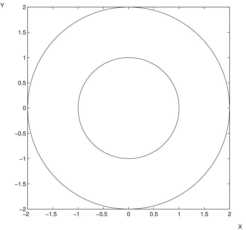
Figure 3.1: A schematic representation of the concentric circular billiard that simulates the reversible reaction $A+B\leftrightarrow C+D$. A narrow opening is assumed to exist on the outside larger circle through which the particles leave the billiard.

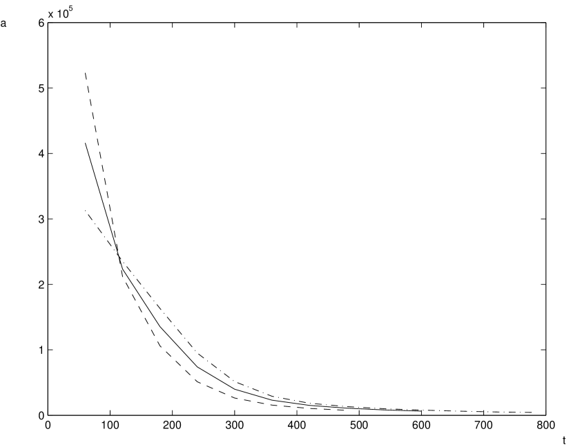
Figure 3.2: The dashed curve shows the activity obtained when all the $10^{6}$ particles of the ensemble are allowed to be only in “state” 2, in which they are reflected between points on the outer circle only. The dashdot curve is the activity when all these particles are allowed to move only in “state” 1 (between the two circles). For the values assigned here to the outer and inner circles (6 and 3) the dashed (dashdot) curve is the maximum (minimum) activity. The solid curve shows the activity obtained when the particles in either state pass to the other after every 1100 reflections. The $x$ axis specifies time binned in units of 60.

Now, since in such a system we can not follow the path of each particle and can not differentiate between the two kinds of motion we have to consider, as done for the nuclear and radioactive processes [71], the activities of these particles in either path. That is, the rate at which the entire ensemble of particles, being at either state, leaves the billiard. We assume for the activity discussed here, as is assumed [71] for the nuclear and radioactive’s activities, that each particle $A$ enjoys arbitrary initial conditions, so in the following numerical simulations we assume that it may begin its journey inside the billiard at either “state” which is determined randomly using a random number generator. As remarked, we want to show, numerically, that if either side of this reversible reaction $A+B\leftrightarrow A+C$ is repeated a large number of times $N$ in a finite total time $T$, then, in the limit of very large $N$, the activity obtained is the same as the “natural activity” [19] that results when no such repetitions are done [19]. For that matter, we take into account that the reversible reactions that occur in nature have either equal or different rates for the two directions of the reactions and that the total activity of such ensemble in which these reactions happen depend critically upon these rates [71]. If, for example, we consider the equal rate case then we have to discuss the rate of evacuation of the billiard when each particle is allowed, after a prefixed number of reflections in either state, to pass, if it is still in the billiard, to the other one. This activity is shown by the solid curve in Figure 3.2 in which the ordinate axis denotes the number of particles $A$ that leave the billiard in prescribed time intervals binned in units of 60 [71]. We assume [71] that each point particle $A$ in either state moves with the same speed of 3, and the hole through which they leave has a width of 0.15. We denote the outer and inner radii of the billiard by $r_{1}$ and $r_{2}$ respectively, and assign them the values of $r_{1}=6$ and $r_{2}=3$. The initial number of the particles $A$ was $10^{6}$, and each one of them passes from one “state” to the other, if it did not leave the billiard through the hole, after every 1100 consecutive reflections. We note that this rate of one passage for every 1100 reflections is typical and common for these kinds of billiard simulations [71, 72]. The natural activity is obtained, as remarked, when the entire ensemble of $10^{6}$ particles $A$ enter, one at a time, the billiard at the same definite “state” and remain all the time in this “state” without passing to the other until they leave the billiard. The dashed curve in Figure 3.2 shows this natural activity when all the particles $A$ are in “state” 2 in which they are reflected only between points of the outer circle untill they leave the billiard. The dash-dot curve shows the activity when all the particles $A$ are in “state” 1 in which they are reflected only between the two circles. It has been found that for the values assigned here to the radii of the outer and inner circles (6 and 3) the activity of “state” 2 shown by the dashed curve is the maximum avilable and that of state 1 shown by the dashdot curve is the minimum. The large difference between the two activities has its source in the range of the allowed angles of reflections which is much larger in state 2 than in state 1. This is because the minimum trajectory between two neighbouring reflections in state 2, where the particles $A$ are reflected between points of the outer circle only, may be infinitesimal compared to the corresponding trajectory in state 1 which is (we denote the trajectories between neighbouring reflections in states 1 and 2 by $d_{1}$ and $d_{2}$ respectively) $d_{1_{min}}=r_{1}-r_{2}$. For the values assigned here to the radii $r_{1}$ and $r_{2}$ of the two concentric circles ($r_{1}=6$ and $r_{2}=3$) $d_{1_{min}}=3$. We note that the maximum trajectory between two neighbouring reflections in state 2 is equal to the corresponding one in state 1, that is

$$d_{1_{max}}=d_{2_{max}}=\sqrt{r_{1}^{2}+r_{2}^{2}}$$

Thus, the particles in $A$ have many more possibilities to be reflected to the hole and leave the billiard in state 2 than in state 1 and, accordingly, their activity is much larger. The solid curve in Figure 3.2 is, as remarked, the activity obtained when the particles $A$ are transferred between the two states at the rate of one passage for every 1100 reflections and so, as expected, its activity is between the two other activities shown in Figure 3.2.

We numerically interfere with the rate of the systematic passage of the point particles $A$ between the two states such that this rate is accelerated. It is found that the activity of the entire ensemble is directly (inversely) proportional to the rate of the passage from state 1 (2) to state 2 (1) when the opposite passage from state 2 (1) to state 1 (2) remains at the rate of one for every 1100 reflections. Thus, we have found that when the particles in state 1 (2) are transferred to state 2 (1) at the maximum rate of one passage after each single reflection and the particles in state 2 (1) are passed to the state 1 (2) at the rate of one for every 1100 reflections then the activity of the particles $A$ is maximal (minimal). But as we have remarked the maximal (minimal) activity is obtained only when each particle of the entire ensemble is always in state 2 (1). In other words, as we have remarked, a very large number of repetitions of the left (right) direction $A+B\to A+C$ ($A+C\to A+B$) of the reaction where the right (left) direction $A+C\to A+B$ ($A+B\to A+C$) occurs every 1100 reflections, yields a result as if the densely repeated reaction never happened and the activity obtained is the natural one in which no repetition is present. The dashed curve in Figure 3.3, which is the same as the dashed one of Figure 3.2, shows the activity obtained when all the $10^{6}$ particles $A$ of the ensemble are allowed to move only in state 2 until they leave the billiard. The solid curve is the activity obtained when the reaction $A+C\to A+B$ is repeated after each single reflection and the opposite one $A+B\to A+C$ after every 1100 reflections.

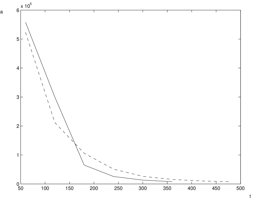
Figure 3.3: The dashed curve, which is the same as the dashed curve of Figure 3.2 (they look slightly different since the abcissa axes of these figures are different), shows the activity obtained when all the $10^{6}$ particles $A$ of the ensemble are numerically constrained to be only in “state” 2 until they evacuate the billiard. State 1 is not allowed for them. The solid curve is the activity obtained when each particle in state 1 is passed to “state” 2 after each single reflection, whereas those in “state” 2 pass to the opposite one only after every 1100 reflections. As for Figure 3.2 the abcissa axis denotes time binned in units of 60. Note the similarity between the two curves.

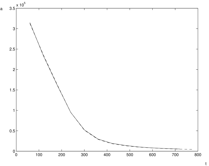
Figure 3.4: The apparently one curve shown in the figure is actually two curves one dashed and the other solid. The dashed curve, which is the same as the dashdot curve of Figure 3.2, shows the activity obtained when all the $10^{6}$ particles $A$ of the ensemble are numerically constrained to be only in “state” 1 until they evacuate the billiard. State 2 is not allowed for them. The solid curve is the activity obtained when each particle in state 2 is passed to “state” 1 after each single reflection, whereas those in “state” 1 pass to the opposite one only after every 1100 reflections. As for Figure 3.2 the abcissa axis denotes time binned in units of 60. Note that the two curves are almost identical (the dashed curve has a longer tail (for large $t$) than the solid one).

It is seen that the curves of Figure 3.3 are similar to each other. That is, the results obtained are in accordance with the former sections where a large number of repetitions of the reaction yields a result that characterizes the activity obtained in the absence of such repetitions. This is seen, in a much more clear way, in Figure 3.4 for the other direction $A+B\to A+C$ of the reaction. The apparent single graph of the figure is actually composed of two curves; one solid and the other dashed. The solid curve shows the activity obtained when the reaction $A+B\to A+C$ is repeated after each single reflection and the opposite one $A+C\to A+B$ after every 1100 reflections. The dashed curve, which is identical to the dash-dot one from Figure 3.2, is the activity obtained when all the particles $A$ of the ensemble are constrained to move only in state 1 until they leave the billiard. Note that the two curves are almost the same except for the longer tail of the dashed curve.

From both Figures 3.3 and 3.4 we realize that the large number of repetitions of either direction of the reversible reaction $A+B\leftrightarrow A+C$ has the effect as if it has not been performed at all and the actual activity obtained is that of the natural one that does not involve any repetitions.

We note that as the analytical results are obtained in the limit of the largest number (actually infinite) of repetitions so the similar numerical results are obtained in the limit of the largest number of repetitions of the reaction. That is, of numerically repeating it after each single reflection. In other words, a mere high rate (which is not the maximal) of one side of the reaction compared to the slow one is not enough to produce the results shown in Figures 3.3-3.4. This is clearly shown by the solid curve in Figure 3.5 which shows the activity obtained when each particle in “state” 1 is passed to “state” 2 after every two consecutive reflections (the high frequency reaction) whereas those of “state” 2 are passed (one at a time) after every 1100 reflections (the low frequency reaction).

Figure 3.5: The dashed curve, which is the same as the dashed curve of Figure 3.3, shows the activity obtained when all the $10^{6}$ particles $A$ of the ensemble are moving inside the billiard only in “state” 2 until they are evacuated outside of it. State 1 is not allowed for them. The solid curve is the activity obtained when each particle in state 1 is passed to “state” 2 after every two reflection, whereas those in “state” 2 pass to the opposite one only after every 1100 reflections. Note that although the two solid curves of Figures 3.3 and 3.5 are obtained under almost the same conditions the activities are very different (see text). As for all the former figures the abcissa axis denotes time binned in units of 60.

Note that the solid curve in Figure 3.3 shows the activity obtained when the particles in “state” 1 are passed to “state” 2 after each reflection and those of 2 passed to 1 after every 1100 reflections. That is, although the two high rates represented by the two solid curves in Figures 3.3 and 3.5 are almost the same nevertheless the resulting activities, contrary to what one may expect, are very different. That is, that of Figure 3.3 is much higher than that of Figure 3.5 as may be seen from the solid curve that begins at $t=60$ (note that our abcissa axis is binned in units of 60) from the high value of $5.65\cdot 10^{5}$ and ends at $t=360$. The corresponding solid curve of Figure 3.5 begins at $t=60$ at the much smaller value of $4.45\cdot 10^{5}$ and ends at the later time of $t=420$. That is, by only increasing the rate of repeating the same reaction from one for every two reflections to one for each reflection results in an additional 120000 particles that leave the billiard already at the first binned time unit. The two dashed curves of Figures 3.3 and 3.5 are identical and denote the same activity obtained when all the $10^{6}$ particles $A$ of the ensemble are numerically constrained to be only in “state” 2 until they evacuate the billiard. Thus, as remarked, the important factor that causes a result of maximum activity is the highest possible rate and not merely a large ratio between the higher and slower frequencies. This is in accord with the analytical results obtained in Sections 3.2 and 3.3 in which the largest rate (actually infinite) of repeating the same direction of the general reversible reaction $A_{1}+A_{2}+\cdots A_{r}\leftrightarrow B_{1}+B_{2}+\cdots+B_{s}$, where $r$, $s$ are any two arbitrary natural positive numbers, yields the results of remaining with a unity probability with the initial reacting particles as if the repeated reaction did not occur at all.

All the former simulations were done when the outer and inner circles radii were 6 and 3 respectively. We note that we obtain similar numerical results for all other assigned values of $r_{1}$ and $r_{2}$ up to the extreme limits of $r_{1}>\!>r_{2}$ and $r_{1}\approx r_{2}$ provided we always have $r_{1}>r_{2}$.

These results may be explained along the same line used to interpret the similar results obtained analytically [2, 11, 12, 13, 14] and experimentally [10] in the quantum regime. That is, a quantum system, which may reduce through experiment to any of its relevant eigenstates, is preserved in its initial state by repeating the experiment of checking its state a large number of times in a finite total time which is the static Zeno effect [2, 10, 11, 12, 13, 14]. The similar results obtained theoretically in Section 3.2 suggest that this effect may be effective also in the classical reactions. That is, repeating them a large number of times, in a finite total time, may result in remaining with the initial reacting particles as if the repeated reaction did not happen at all. Moreover, the dynamic Zeno effect [11, 12] may also be obtained as in Section 3.3, in which we show that the joint probability density for the occurence of $n$ special different reactions between the initial and final times $t_{0}$ and $t$ tends to unity in the limit of $n\to\infty$. The Zeno effect has been shown also in the numerical simulations from which we realize that repeating a large number of times any direction of the reversible reaction $A+B\leftrightarrow A+C$ has, in the limit of numerically repeating it after each single reflection, the effect as if it has never happened and the activity obtained is the natural one in which no repetitions occur. That is, the very large number of repetitions, in a finite total time, causes the resulting activity to be the same as if these repetitions never happened as obtained in the Zeno effect in which the system is preserved in the initial state due to the very large number of measurements.

We see, therefore, that the large number of repetitions of either the same reaction (corresponds to the static Zeno effect), or along a consecutive sequence of different ones (corresponds to the dynamic Zeno effect) causes the relevant system, as seen in the former chapters, to respond differently compared to its response in the absence of these repetitions. That is, referring to the first case we see that although the related reaction is done a very large number of times one remains with the initial reacting particles only as if no reaction has ever been done. For the second case the new response, as a result of these dense reactions along the specific path of reactions, is to “realize” this path so that the probability to proceed along these reactions is unity. That is, we see for both cases that the mere act of repetitions of the kind involved changes the behaviour of the system to an entirely new and unexpected one. Moreover, we can at any time reconstruct this unexpected response of the system by going once more through the dense repetitions process. That is, under the condition of dense measurement we may establish and validate these new responses of the system. Note that exactly the same results were obtained in Chapter 2 with respect to the quantum field examples discussed there. We will also obtain the same results in the following Chapters of this work. These unique effects of the dense repetitions have also been, numerically, shown using the circular billiard model [19].

Chapter 4 Space Zeno effect

4.1 Introduction

The effect of performing the same experiment simultaneously in a very large number of regions of space all occupying a finite space is similar to that of performing an experiment repetitively a large number of times in a finite interval of time. The difference is that the repetition in the second case is over independent units of equal steps in time, while in the first case it is over independent units of equal shifts in space. We have shown [23] that as the Zeno effect [2, 10, 11, 12, 13, 14] is obtained in the second case when these equal intervals of time tend to infinitesimal values, so this effect occurs also in the first case when the equal shifts in space tend to be infinitesimal.

Piron has discussed in [73] a physical example of how this procedure can be seen as an actual evolution. He considers an array of Geiger counters at each of a closely spaced set of points along the $x$ axis. This type of apparatus treats the value of $x$ at which an event occurs as a classical parameter, since the $x$ value of each counter is known in advance. What is unknown is the time $t$ at which the counter will trigger, and this $t$ then becomes a quantum observable. Passing from a counter at $x$ to a counter at $(x+\rho)$ corresponds to a Hamiltonian type evolution $e^{-\frac{ip_{1}\rho}{\hbar}}$, generated by the evolution operator $p_{1}$, now a function on the phase space $(H,t,y,z,p_{y},p_{z})$. The survival amplitude is $(\phi_{x_{0}},e^{-ip_{1}\rho}\phi_{x_{0}})$, with $\phi_{x_{0}}(t,y,z)$ some “initial” state at position $x_{0}$. The successive performances of such experiments along the $x$ axis at small intervals $\frac{X}{n}$, as $n\to\infty$ corresponds precisely to the analogous process of the time Zeno effect. Since, in this limit, the state $\phi_{x_{0}}$ is stabilized (as for the time Zeno effect), the distribution in $t$, $y$, and $z$ becomes stationary, and we see that the effect is that of essentially “simultaneous” (at the peak $t$) measurements over an interval of $x$.

As pointed by Piron [73] the two formulations, 1) according to the parameter $t$ (as in a bubble chamber type of experiment where $t$ is known, but the locations $x$, $y$, and $z$ are subject to measurement), and 2) according to the parameter $x$ (as in the set of Geiger counters described above, where the $x$ is determined, but the times $t$ at which the counters are triggering are the results of measurement) are classically completely equivalent, as can be seen by a change of variables. In the quantum case, the difference is profound, i.e, in the first case $t$ is an evolution parameter and $x$, $y$, $z$ are physical observables, while in the second case, $x$ is the parameter of evolution, and $t$, $y$, $z$ are the observables. Our comparison here of the two interpretations corresponds to a qualitative equivalence which carries over, under suitable conditions, to the quantum theory.

In Section 4.2 we show, using Appendix $C_{1}$, that the suitable expression for the space Zeno effect may be obtained by exchanging the time and space variables and making the necessary changes. In Section 4.3 we demonstrate, by referring to different articles [17, 18, 20, 21, 52], the existence of the spatial Zeno effect in both quantum and classical systems and by this we show that it is a general effect and not only a quantum one. We have just shown in Chapter 3 that it may be found also in chemical classical reactions.

4.2 A coherent and general state examples of the space Zeno effect

As seen from [23] one may obtain the relevant analytical expressions for the space Zeno effect by substituting the time variable $t$ by the space variable $r$ and doing the resulting necessary changes. This may be seen from Eqs (1)-(9) of [23] ( Sections 1-3 of which are shown in Appendix $C_{1}$). These equations discuss the specific case of the ground state of the harmonic oscillator $\phi(x)=({w\over\hbar\pi})^{1\over 4}e^{-{1\over 2\hbar}wx^{2}}$ and demonstrate the kind of transfer one do from the time variable to the spatial one. The more general case is also discussed (see Eqs (9)-(11) in [23] and in Appendix $C_{1}$) and one may see the appearance of the space Zeno effect in the limit of $n\to\infty$ where $n$ is the number of systems (observers) in the finite spatial section that perform these experiments.

4.3 The one-dimensional arrays of the multibarrier potential and multitrap systems of finite range

We refer in the following to the articles [17, 18, 20, 21, 52] which discuss the quantum and classical systems of the one dimensional arrays of multibarrier potential and multitraps systems of finite ranges. In [18] the quantum one-dimensional multibarrier potential of finite range is discussed, and in [20] the corresponding classical multitrap system. We may see that although these two systems are entirely physically different and necessitate different methods of analysis as should be for quantum and classical systems, nevertheless, they clearly show the same somewhat unexpected behaviour. That is, as the number of either the quantum potential barriers or the classical traps increases the value of the respective probability amplitude or the classical density after crossing these systems tend to remain in their former values before passing them. This behaviour is contrary to what one may expect that the values of the former variables must decrease with increasing the number of barriers or traps. This is shown explicitly in Appendices $C_{2}$ and $C_{3}$ in which we represent respectively the relevant paper [18] and Sections 1-2 of [17] for the one-dimensional multibarrier potential of finite range and in Appendix $C_{4}$ which shows the paper [20] for the corresponding one-dimensional multitrap system.

In the two systems one sees the same correspondence not only for a variable total length of each [17, 20] but also for a constant length. Moreover, the same parameter $c=\frac{b}{a}$, which denotes in both systems [17, 18, 20, 21, 52] the ratio of the total interval between the barriers or traps to their total length, has turns out to have the same influence in these two different systems. Both papers [18, 20] use the transfer matrix method [74, 75] to obtain analytical expressions for the relevant transmission probability or the classical density in the respective limits of infinite number of barriers or traps which are the limits for which the space Zeno effect appears. In Section 4.4 we show that both systems behave the same also for the case of finite number $N$ of potential barriers or traps and, especially, in the transfer to large $N$. For this we use, for both systems, numerical simulations in contrast to the explicit expression we have obtained fot the $N\to\infty$ case. In the following section we use the numerical $4n\times 4n$ matrix approach which is applicable for both systems.

4.4 The $4n\times 4n$ matrix approach

We, now, show that both one-dimensional systems of quantum potential barriers and classical traps demonstrate the same behaviour also for finite number of barriers and traps and especially in the transfer to the large numbers of them. The quantum case has already been discussed in [17] and the relevant Sections are appended to Appendix $C_{3}$. We, now, show the same behaviour also for the multitrap system by starting from Eqs (7)-(10) in [20] (appended to Appendix $C_{4}$) which are valid for the first trap. Continuing in the same manner for all the other $n-1$ traps we obtain $4n$ simultaneous equations with $4n+2$ unknowns $A,B,C,\ldots$ etc. Now, since these $4n$ simultaneous equations are not sufficient to determine the $4n+2$ unknowns we must reduce the number of the unknown variables from $4n+2$ to $4n$ by using the following two assumptions: (1) Noting that the traps act as imperfect ones (see the original problem from the set (1) in [20]) we divide all the $4n$ equations by the value of the coefficient of the density function of the imperfect problem at the left hand side of the first trap. That is, this is the value of the coefficient of the density of the diffusing particles before their interaction with the traps. (2) The second assumption is that at the point $x=a+b$ at the right hand side of all the $n$ traps we ignore the ideal trap component of the density function since it is clear that the density of the particles that survive the $n$ traps can not be represented by any ideal trap function. We remark that these two assumptions of dividing by some nonzero unknown and ignoring another in order to equate the number of unknown variables to the number of equations are common in the literature (see, for example, the potential barrier problem in [37] and [74]). These two assumptions reduce the number of unknown variables to $4n$, and so they can be determined by the $4n$ equations. We denote the ideal and imperfect trap components by $\rho_{1}(D,x,t)$, and $\rho_{2}(D,x,t)$ respectively where $D$ is either the external diffusion constant outside the traps in which case it is denoted by $D_{e}$ or inside them whereby its notation is $D_{i}$. The notation $\grave{\rho}$ denotes the first derivative of the density function $\rho$ with respect to the $x$ variable. The $4n$ simultaneous equations system is, therefore, given by

$$\rho_{2}(D_{e},\frac{b}{n},t)=C\rho_{2}(D_{i},\frac{b}{n},t)$$

$$\grave{\rho}_{2}(D_{e},\frac{b}{n},t)+B\grave{\rho}_{1}(D_{e},\frac{b}{n},t)=C\grave{\rho}_{2}(D_{i},\frac{b}{n},t)+D\grave{\rho}_{1}(D_{i},\frac{b}{n},t)$$

$$C\rho_{2}(D_{i},\frac{a+b}{n},t)=E\rho_{2}(D_{e},\frac{a+b}{n},t)$$

$$C\grave{\rho}_{2}(D_{i},\frac{a+b}{n},t)+D\grave{\rho}_{1}(D_{i},\frac{a+b}{n},t)=E\grave{\rho}_{2}(D_{e},\frac{a+b}{n},t)+F\grave{\rho}_{1}(D_{e},\frac{a+b}{n},t)$$

$$......................................................................$$

$$.........................................................................$$ (4.1)

$$.........................................................................$$

$$R\rho_{2}(D_{e},\frac{(n-1)a+nb}{n},t)=T\rho_{2}(D_{i},\frac{(n-1)a+nb}{n},t)$$

$$R\grave{\rho}_{2}(D_{e},\frac{(n-1)a+nb}{n},t)+S\grave{\rho}_{1}(D_{e},\frac{(n-1)a+nb}{n},t)=$$

$$=T\grave{\rho}_{2}(D_{i},\frac{(n-1)a+nb}{n},t)+U\grave{\rho}_{1}(D_{i},\frac{(n-1)a+nb}{n},t)$$

$$T\rho_{2}(D_{i},a+b,t)=V\rho_{2}(D_{e},a+b,t)$$

$$T\grave{\rho}_{2}(D_{i},a+b,t)+U\grave{\rho}_{1}(D_{i},a+b,t)=V\grave{\rho}_{2}(D_{e},a+b,t)$$

The last set (4.1) can be written as the matrix equation

$$Nx=c,$$

where $N$ is the square matrix with $4n$ rows and $4n$ columns, $x$ is the unknown vector with the $4n$ unknowns $(B,C,\cdots T,U,V)$ and $c$ is the constant vector whose first two elements are $-\rho_{2}(D_{e},\frac{b}{n},t)$ and $-\grave{\rho}_{2}(D_{e},\frac{b}{n},t)$, and all its other $(4n-2)$ elements are zeroes. $a$ is the total width of the traps and $b$ is the total interval among them [20]. Note that the last set is very similar in form to the corresponding sets of the quantum case (see the sets (1) and (3) in [17]) and like them can be managed, especially for large $n$, only by numerical simulations. We can compute, numerically, each one of the $4n$ variables not only for constant $a$, $b$, and $n$, but also can determine how each of these variables behaves as a function of $a$ for constant $n$, or as a function of $n$ for constant $a$ (usualy $b=a$, or $b=\frac{a}{2}$). Typical values of the diffusion constant are conventionaly found in the literature in the cgs units and range from $0.1\frac{(cm)^{2}}{sec}$ to $0.8\frac{(cm)^{2}}{sec}$ [77]. At $t=0$ we find that $V$ (see the set (4.1)), which is the ratio of the imperfect trap density function coefficient at the point $x=a+b$ (after passing the $n$ trap system) to that at the point $x=\frac{b}{n}$ (before passing it) is unity for all values of $n$ and $a$. We have obtained this result for $k=1$, $D_{e}=0.5$, $D_{i}=0.1$ and $b=\frac{a}{2}$. That is, at the initial time the densities at the two extreme sides of the trap system are equal. When $t$ departs from zero the coefficient $V$ becomes smaller for the same values of $n$ and $a$. That is, as time progresses the density after the $n$ trap system becomes smaller than that before it as expected from a physical point of view.

The interesting and unexpected findings, obtained analytically and numerically, are found when the number $n$ of either the potential barriers in the quantum system or traps in the classical one increases. In this case the respective probability amplitude or the particle density grows so that in the limit $n\to\infty$ both variables tend to the initial value they have before passing through the systems. That is, contrary to what one may expect the larger is the number of barriers or traps the easier will be for the entire ensemble of particles (quantum or classical) to pass through them. That is, we see, as remarked, that experimenting uninterruptedly on either a quantum or a classical system totally changes the known response of these systems to that of a new, even unexpected, one. Moreover, as remarked in the former parts of this work with respect to the bubble and open-oyster examples (as well as the programming examples of [9, 51]) we may cause these systems to repeat, as many times as we wish, their new and unexpected behaviours by experimenting again with them in a dense manner. In other words, by this kind of dense experimenting we may establish and validate these new and unexpected responses of these systems. Note that, as we have remarked in Section 1.2, we do not have to reach the limit of $n\to\infty$ or even large $n$ in order to obtain again these new responses (new phenomena) of these systems. As seen in [17, 20, 21] (see Appendices $C_{2}$, $C_{4}$, $C_{5}$ and the figures there) one does not have to take more than 30 barriers (even less for the case of traps as seen in [21] (see Appendix $C_{5}$)) for obtaining a significant transmission of the respective quantum or classical particles. These large transmissions constitute, as remarked, the new phenomena that may be repeated by preparing again these 30 barriers.

The establishing effect that results from the space Zeno effect where a large number of similar systems, confined in a finite region of space, perform similar experiments turns our attention to directly consider the effect of a large ensemble of related observers. We do this in the following chapter.

Chapter 5 The effects of the ensemble of related observers in quantum and classical phenomena

5.1 Introduction

In this chapter we discuss the influence of observation and observers upon the obtained experimental results and although the effect of these have been discussed in the literature [8] (see also [5] and references therein) a little was said regarding the influence upon the obtained results of the presence or absence of mutual relationship and cooperation among them. We concentrate our discussion here to the effects that result when a large ensemble of related observers perform experiments. By the term "related observers" we mean that the members of the ensemble are related to each other by some kind of connection such as, for example, that each one of them do his experiment on the same kind of system as all the others. The last condition ensures that any result obtained by any one of them are valid for all the others in the sense that if the relevant experiment is repeated, under the same conditions, by any other member of the ensemble the results obtained will be the same. This will not be the case for the unrelated observers that do not have the same kind of systems so they can not perform the same experiment under the same conditions. Thus, the results obtained by any one of them are valid only for the specific involved system and not for the other different ones.

We note that when the observers of the ensemble participate in some collective experiment then the relation among them is established not only by having the same kind of systems but also by the degree of their mutual cooperation in the experiment. Thus, they will be maximally correlated if they perform the collective experiment in such a way that not two of them prepare and do their specific parts independently of each other. This kind of connection among the members of the ensemble will be analytically discussed in Sections 5.2 and 5.4. We show that the probability for the physical validation of real phenomena increases for large number of related observers and this is obtained for the whole of them without having each one doing dense measurement along the specific Feynman paths that represent these phenomena.

In Section 5.2 we use the Feynman path integral method [30, 31, 32] to show this behaviour and in Section 5.3 use is made, for this purpose, of Everett’s relative state theory [53, 54]. We show, using the unique character of the last theory, that the number of observers increases in an asymptotic manner as the number of experiments grows as seen from the following Eq (5.8) and Table 1. For example, for 100 experiments we have over $10^{306}$ different observers. Both theories, together with Figures 5.1-5.3 and Table 1, clearly demonstrate that the presence of a large ensemble of related observers not only makes possible the resulting physical validation of real phenomena but it is more enabled the larger is the ensemble. This does not hold for the ensemble of unrelated observers or for the single one as will be shown. Note that the appearance of physical reality for the large number of identical systems all prepared in the same initial states have already been discussed in the literature [27, 78, 79] from different points of view. As remarked, we discuss also in this work the case where the large ensemble of systems was aligned in such a way that no two of them are prepared in the same initial state (see, especially, Sections 5.2 and 5.4).

In Section 5.4 we show, using the classical thermodynamical system of cylinder and pistons [76, 77], that the influence of the ensemble of related observers is effective also in classical systems. Moreover, since this system is simple the effect of the ensemble is shown in a more direct manner. We follow the discussion in [76] and generalize it to include the large ensemble of related observers. That is, we test some assumed relation between the variables of the thermodynamical system and find the conditions under which this relation becomes established or refuted. We follow the whole procedure in [76] of first attempting some initial relation so that if it turns out through experiments that it does not cover all the possible motions of the particles in the cylinder a new and better relation is proposed. We show that the new theory becomes established only for a related large ensemble of observers that perform similar experiments. It is shown that the effect of such a related ensemble of observers is to physically establish the new assumed relation compared to that of an unrelated ensemble that have no effect in this respect.

We note that this obtained effect of the ensemble of observers, compared to that of the single one, is in accordance with the space Zeno effect discussed in the former chapters. That is, when the large ensemble of related observers operate cooperatively any result obtained from any experiment done by any observer of the related ensemble becomes valid for the whole of them. This corresponds to the preserving of the given initial probability amplitude or the particle density in passing respectively through either a large number of a one-dimensional array of potential barriers or traps. This does not hold for the ensemble of unrelated observers or for the single one which corresponds, as remarked, to the time Zeno effect and not to the spatial one. Note that exactly the same results were obtained in [51] with respect to the Internet websites where we see that if the clusters of doubly linked websites are large enough then adding only a small amount of connecting links results in, actually, a phase transition-type strengthening of the overall connectivity among them. This unusual increase of the overall connectivity due to a small addition of it corresponds to the former overall physical realization for the whole ensemble of the result obtained by only one of them.

5.2 The Feynman path integrals of the ensemble of observers

The collective measurement is performed by first preparing $N$ similar systems at $N$ arbitrarily selected states, from actually the very large number which constitute the specific Feynman path of states which we want to “realize” [11, 12] by densely experimenting along it. These systems are then delivered to the $N$ observers of the ensemble so that the system $i$ $(i=1,2,\ldots N)$, prepared at the state $\phi_{i}$, is assigned to the observer $O_{i}$. Thus, we may write for the probability amplitude that the first observer $O_{1}$ finds his system, after doing the experiment of checking its present state, at the state $\phi_{2}$ of the second observer $O_{2}$

$$\Phi_{12}=\sum_{i}\phi_{1i}\phi_{i2}$$ (5.1)

The summation is over all the possible secondary paths [1] (as those shown along the middle path of Figure 5.1) between $\phi_{1}$ and $\phi_{2}$ and the quantities $\phi_{1i}$ and $\phi_{i2}$ denote [30] the probability amplitudes to proceed from the state $\phi_{1}$ to $\phi_{i}$ and from $\phi_{i}$ to $\phi_{2}$ respectively. In the same manner one may write for the conditional probability amplitude that the second observer $O_{2}$ finds his system at the state $\phi_{3}$ (of the observer $O_{3}$), provided that the observer $O_{1}$ finds his system at the state $\phi_{2}$

$$\Phi_{23|12}=\sum_{ij}\phi_{1i}\phi_{i2}\phi_{2j}\phi_{j3}$$ (5.2)

Where $\Phi_{23|12}$ is the remarked conditional probability amplitude and $\sum_{ij}$ is the summation over all the secondary paths that lead from the state $\phi_{1}$ to $\phi_{2}$ and over those from $\phi_{2}$ to $\phi_{3}$. Correspondingly, the conditional probability amplitude that the $(N-1)$-th observer finds his system at the state $\phi_{N}$ of the observer $O_{N}$ provided that all the former $(N-2)$ observers find their respective systems, that were initially prepared at the states $\phi_{i}\ \ (i=1,2,\ldots N-2)$, to be at the states $\phi_{i}\ \ (i=2,3,\ldots N-1)$

$$\Phi_{N-1N|12,23,\ldots,N-2N-1}=\sum_{ij\ldots rs}\phi_{1i}\phi_{i2}\phi_{2j}\phi_{j3}\ldots\phi_{N-2r}\phi_{rN-1}\phi_{N-1s}\phi_{sN}$$ (5.3)

Figure 5.1 shows 7 Feynman paths, from actually a large number of paths that all begin at $\phi_{1}$ and end at $\phi_{8}$ (only 8 states are shown in the figure for clarity). The middle path is the specific one along which the described collective dense measurement is performed.

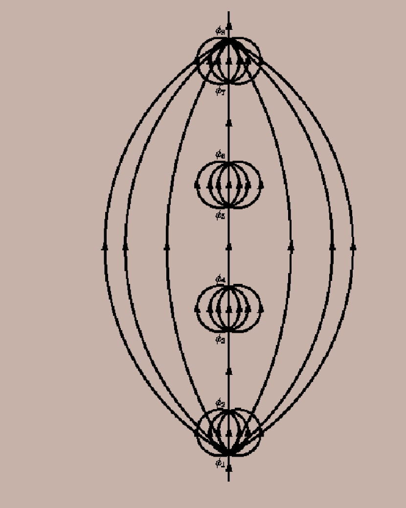
Figure 5.1: seven Feynman paths of states that all begin at the state $\phi_{1}$ and end at $\phi_{8}$ are shown in the figure. The middle path is the one along which the collective dense measurement is performed by the ensemble members $O_{i}\ \ \ i=1,2,\ldots N$. The $N$ separate systems of these observers have been initially prepared in the states $\phi_{i}\ \ \ i=1,2,\ldots N$. Only eight states are shown in the figure for clarity. Note the secondary Feynman paths between neighbouring states in the middle path.

Along this line we have the $N$ ($N=8$ in the figure) initially prepared states $\phi_{1},\phi_{2},\ldots\phi_{N}$ as well as the secondary Feynman paths that lead from each $\phi_{i}$ to $\phi_{i+1}$ where $i=1,2,\ldots,(N-1)$ . The relevant conditional probability is found by multiplying the last probability amplitude from Eq (5.3) by its conjugate to obtain, omitting the subscripts of the $\Phi$’s for clarity

$$\Phi^{\dagger}\Phi=\sum_{\grave{i}\grave{j}\ldots\grave{r}\grave{s}}\sum_{ij\ldots rs}\phi_{\grave{i}1}\phi_{1i}\phi_{2\grave{i}}\phi_{i2}\phi_{\grave{j}2}\phi_{2j}\phi_{3\grave{j}}\phi_{j3}\ldots\phi_{\grave{r}N-2}\phi_{N-2r}\phi_{N-1\grave{r}}\phi_{rN-1}\cdot$$

$$\cdot\phi_{\grave{s}N-1}\phi_{N-1s}\phi_{N\grave{s}}\phi_{sN}=(\sum_{\grave{i}i}\phi_{\grave{i}1}\phi_{1i}\phi_{2\grave{i}}\phi_{i2})(\sum_{\grave{j}j}\phi_{\grave{j}2}\phi_{2j}\phi_{3\grave{j}}\phi_{j3})\ldots$$ (5.4)

$$\ldots(\sum_{\grave{r}r}\phi_{\grave{r}N-2}\phi_{N-2r}\phi_{N-1\grave{r}}\phi_{rN-1})(\sum_{\grave{s}s}\phi_{\grave{s}N-1}\phi_{N-1s}\phi_{N\grave{s}}\phi_{sN}),$$

where the number of all the double sums $\sum_{\grave{i}i}\sum_{\grave{j}j}\ldots\sum_{\grave{r}r}\sum_{\grave{s}s}$ is $N$.

We note that we regard the traversed Feynman path as actually composed of a very large number of states. Thus, no matter how large is the number $N$ of observers there will always be a sufficient number of states to assign to all of them so that no two observers have the same state.

As remarked, we are interested in the limit of dense measurement along the relevant Feynman path in order to realize it so we take $N\to\infty$. In this limit the length of the secondary Feynman paths among the initially prepared $N$ states (where now $N\to\infty$) tends to zero [1] so that the former probabilities to proceed along the secondary paths between the given states become the probabilities for these states. Thus, we may write for Eq (5.4) in the limit of $N\to\infty$

$$\lim_{N\to\infty}<\!\Phi^{\dagger}|\Phi\!>=\lim_{N\to\infty}<\!\phi_{\grave{i}1}|\phi_{2\grave{i}}\!><\!\phi_{i2}|\phi_{1i}\!><\!\phi_{\grave{j}2}|\phi_{3\grave{j}}\!><\!\phi_{j3}|\phi_{2j}\!>\ldots$$

$$\ldots<\!\phi_{\grave{r}(N-2)}|\phi_{(N-1)\grave{r}}\!><\!\phi_{r(N-1)}|\phi_{(N-2)r}\!><\!\phi_{\grave{s}(N-1)}|\phi_{N\grave{s}}\!>\cdot$$ (5.5)

$$\cdot<\!\phi_{sN}|\phi_{(N-1)s}\!>=\delta_{\phi_{\grave{i}1}\phi_{2\grave{i}}}\delta_{\phi_{1i}\phi_{i2}}\delta_{\phi_{\grave{j}2}\phi_{3\grave{j}}}\delta_{\phi_{2j}\phi_{j3}}\ldots\delta_{\phi_{\grave{r}(N-2)}\phi_{(N-1)\grave{r}}}\cdot$$

$$\cdot\delta_{\phi_{r(N-1)}\phi_{(N-2)r}}\delta_{\phi_{\grave{s}(N-1)}\phi_{N\grave{s}}}\delta_{\phi_{sN}\phi_{(N-1)s}}=1$$

The last result of unity follows because in the limit of $N\to\infty$ successive states differ infinitesimally from each other so we may write as in [12] $<\!\phi_{\grave{k}-1}|\phi_{\grave{k}}\!>=<\!\phi_{k-1}|\phi_{k}\!>=\delta_{\phi_{\grave{k}-1}\phi_{\grave{k}}}=\delta_{\phi_{k-1}\phi_{k}}\approx 1$.

Thus, we see that performing dense measurement along any Feynman path of states results in its realization in the sense that the probability to proceed through all of its states tends to unity. Moreover, as described, the dense measurement is performed through the joint action of all the members of the ensemble without having to perform it separately by each one of them. Thus, even when each observer performs his experiment only once, nevertheless, when $N\to\infty$ the obtained realized path is now for all them. Figure 5.2 shows a schematic representation of the state of the ensemble after the remarked collective dense measurement. Each separate batch of 4 similar curves denotes a member of the ensemble that has, as known, a large number of different possible Feynman paths (only 4 are shown for clarity). In the middle part of the figure we have a large number of different batches of paths all mixed among them so it becomes difficult to discern which curve belongs to which batch. The emphasized path in Figure 5.2 is the definite Feynman path along which the described collective dense measurement has been done. Note that this path, actually, belongs to all the different interwoven batches which means that although each one of the observers performs his experimental part only once, nevertheless, after completing the described collective measurement each one of those that participates in it has now the same realized Feynman path. The reason is that although each observer $O_{i}$ of the ensemble performs his experiment on only his specifically prepared state $\phi_{i}$, nevertheless, the results he obtains are valid for all the others since any other observer that acts on the same state $\phi_{i}$ under the same conditions obtains the same result. In other words, the realized Feynman path has been made tangible and real for all of them in the sense that the probability for each to move along its constituent states tends to unity as seen from Eq (5.5).

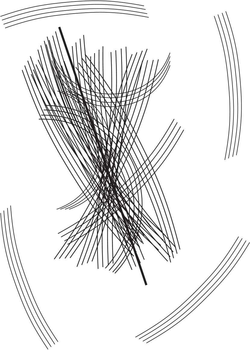
Figure 5.2: A schematic representation of the physical situation after performing the collective dense measurement symbolized by Figure 5.1. Note that although no member of the ensemble has done dense measurement by himself, nevertheless, the joint action of all or most of the observers has resulted in “realizing” the specific Feynman path from Figure 5.1 for all the participating observers. This "realized" path is shown emphasized in the figure.

We note that using the large ensemble of similar systems for analysing experimental results has been fruitfully done in the literature [27, 54, 78, 79]. It has been shown, for example, that considering an $N$ identical systems all prepared in the same initial state one may derive the probability interpretation of quantum mechanics in the limit of $N\to\infty$. That is, this probability is not imposed upon the theory as an external assumption as done in the conventional Copenhagen interpretation of quantum mechanics but is derived from other principles of quantum mechanics [79]. This is done using Finkelstein theorem [78, 79].

5.3 The relative state theory of Everett

The last results may be demonstrated in a more natural and appealing manner by using the relative state theory of Everett [53, 54] that has been formulated, especially, for taking observers into account. We use, in the following, the special notation and terminology of this theory. Thus, if the initial state was some eigenstate of an operator $A$ the total initial state of the (system $S$ $+$ observer $O$) is denoted by $\Psi^{S+O}=\phi_{i}\Psi^{O}[...]$, where $\phi_{i}$ is the initial eigenstate of the system $S$ and $\Psi^{O}[...]$ denotes the observer’s state before the measurement. After the experiment the observer’s state is denoted by $\Psi^{O}[...\alpha_{i}]$, where $\alpha_{i}$ stands for recording of the eigenvalue $\phi_{i}$ by the observer so that the total final state of the (system $S$ $+$ observer $O$) is $\Psi^{S+\grave{O}}=\phi_{i}\Psi^{O}[...\alpha_{i}]$. Now, if the initial state of the system is not an eigenstate but a superposition of them $\sum_{i}a_{i}\phi_{i}$ then the total states before and after the measurement are [53, 54] $\Psi^{S+O}=\sum_{i}a_{i}\phi_{i}\Psi^{O}[...]$, and $\Psi^{S+\grave{O}}=\sum_{i}a_{i}\phi_{i}\Psi^{O}[...\alpha_{i}]$ respectively where $a_{i}=<\!\phi_{i}|\Psi^{S+O}\!>$. Suppose we continue our experiments and measure some other physical observable $B$ beginning from the state $\sum_{i}a_{i}\phi_{i}\Psi^{O}[...\alpha_{i}]$ as the initial one. In such a case one may expand the eigenfunction $\phi_{i}$ of the observable $A$ in terms of the eigenfunctions of $B$ $\phi_{i}=\sum_{j}b_{ij}\phi_{j}$ so that the state $\sum_{i}a_{i}\phi_{i}\Psi^{O}[...\alpha_{i}]$ before the new experiment may be written as [53]

$$\Psi^{S+O}=\sum_{j}\sum_{i}b_{ij}a_{i}\phi_{j}\Psi^{O}[...\alpha_{i}],$$ (5.6)

where $\phi_{j}$ are the eigenfunctions of the operator $B$. After measuring $B$ one obtains

$$\Psi^{S+\grave{O}}=\sum_{j}\sum_{i}b_{ij}a_{i}\phi_{j}\Psi^{O}[...\alpha_{i},\beta_{j}],$$ (5.7)

where $b_{ij}=<\!\phi_{j}|\phi_{i}\!>$ and $\Psi^{O}[...\alpha_{i},\beta_{j}]$ denotes that now the observer records the eigenfunctions $\alpha_{i}$ and $\beta_{j}$ after the two experiments. Continuing and measuring, for example, $n$ observables one obtains the following wave function

$$\Psi^{S+\grave{O}}=\sum_{k}\sum_{l}\sum_{h}\ldots\sum_{j}\sum_{i}c_{hl}d_{lk}\ldots a_{i}\phi_{k}\Psi^{O}[\alpha_{i},\beta_{j},\ldots,\lambda_{l},\xi_{k}],$$ (5.8)

where $c_{hl}=<\!\phi_{l}|\phi_{h}\!>$, $d_{lk}=<\!\phi_{k}|\phi_{l}\!>$, and $\phi_{i}$, $\phi_{j}$ $\ldots$ are eigenfunctions of the $A$, $B$, $\ldots$ operators. Note that each term in Eq (5.8) denotes an observer with his specific sequence $[\alpha_{i},\beta_{j},\ldots,\lambda_{l},\xi_{k}]$ that results from the $n$ experiments. Thus, Eq (5.8), termed the Everett’s universal wave function [53, 54], yields all the possible results that may be obtained from measuring the $n$ observables. We, now, count the number of observers that have the same or similar sequences $[\alpha_{i},\beta_{j},\ldots,\lambda_{l},\xi_{k}]$ which record, as remarked, the $n$ measured eigenvalues. For this we assume that each measurement of any of the $n$ observables may yields $K$ possible different results where the $n$ observables do not have to be all different and so some eigenvalues in the sequence $[\alpha_{i},\beta_{j},\ldots,\lambda_{l},\xi_{k}]$ may be identical. Thus, denoting by $R_{1},R_{2},\ldots,R_{r}$ the numbers of times the $r$ particular eigenvalues $l_{1},l_{2},\ldots,l_{r}$ appear respectively in some specified sequence $[\alpha_{i},\beta_{j},\ldots,\lambda_{l},\xi_{k}]$ we may see from Eq (5.8) that each possible value of $R_{i}$ in the range $0\leq R_{i}\leq n$, and for each $i\ \ \ (1\leq i\leq r)$, may be realized in some observer. Now, the number of sequences in which $l_{1},l_{2},\ldots,l_{r}$ occur, respectively, at $R_{1},R_{2},\ldots,R_{r}$ predetermined positions is $(K-1)^{(n-\sum_{i=1}^{i=r}R_{i})}$ since for each position in the sequence $[\alpha_{i},\beta_{j},\ldots,\lambda_{l},\xi_{k}]$ in which $l_{1},l_{2},\ldots,l_{r}$ are absent there are $(K-1)$ possibilities (note that each position is related only to its specific observable and so to, at most, only one of the $l$’s). Thus, the total number of sequences in which $l_{1},l_{2},\ldots,l_{r}$ occur respectively in $R_{1},R_{2},\ldots,R_{r}$ positions (we denote this number by $N_{l_{1},l_{2},\ldots,l_{r}}$) is

$$N_{l_{1},l_{2},\ldots,l_{r}}=\left(\begin{array}[]{c}n\\ R_{1}\end{array}\right)\left(\begin{array}[]{c}(n-R_{1})\\ R_{2}\end{array}\right)\left(\begin{array}[]{c}(n-(R_{1}+R_{2}))\\ R_{3}\end{array}\right)\ldots$$ (5.15)

$$\ldots\left(\begin{array}[]{c}(n-\sum_{i=1}^{i=r-1}R_{i})\\ R_{r}\end{array}\right)(K-1)^{(n-\sum_{i=1}^{i=r}R_{i})},$$ (5.18)

where $\left(\begin{array}[]{c}n\\ R_{1}\end{array}\right)$ is the number of possible ways to choose in the $n$ member sequence $[\alpha_{i},\beta_{j},\ldots,\lambda_{l},\xi_{k}]$ $R_{1}$ places for $l_{1}$, $\left(\begin{array}[]{c}(n-R_{1})\\ R_{2}\end{array}\right)$ is the number of possible ways to choose $R_{2}$ places from the remaining $(n-R_{1})$ etc. The calculation in Eq (5.15) was done for the more simple case in which all the $l_{1},l_{2},\ldots,l_{r}$ are different. The relevant measure may be found [54] by taking into consideration the expected relative frequency of the eigenvalues $l_{1},l_{2},\ldots,l_{r}$ which is $P_{l_{1},l_{2},\ldots,l_{r}}=|\!\!<\!\Psi_{l_{1},l_{2},\ldots,l_{r}}|\Psi\!>\!\!|^{2}$, where $|\Psi_{l_{1},l_{2},\ldots,l_{r}}\!>$ is the state in which the eigenvalues $l_{1},l_{2},\ldots,l_{r}$ occur among those of the sequence $[\alpha_{i},\beta_{j},\ldots,\lambda_{l},\xi_{k}]$, and also the corresponding relative frequency of any other eigenvalue $m$ different from $l_{1},l_{2},\ldots,l_{r}$, which is $Q_{m}=\sum_{m\neq l_{1},l_{2},\ldots,l_{r}}|\!\!<\!\Psi_{m}|\Psi\!>\!\!|^{2}=1-P_{l_{1},l_{2},\ldots,l_{r}}$. That is, the measure of all the sequences that have the eigenvalues $l_{1},l_{2},\ldots,l_{r}$ at $R_{1},R_{2},\ldots,R_{r}$ predetermined positions respectively is $P_{l_{1},l_{2},\ldots,l_{r}}^{\sum_{i=1}^{i=r}R_{i}}Q_{m}^{(n-\sum_{i=1}^{i=r}R_{i})}$. The last expression must be multiplied by the number of possible ways to choose first $R_{1}$ places for $l_{1}$ from the $n$ positions of the sequence $[\alpha_{i},\beta_{j},\ldots,\lambda_{l},\xi_{k}]$, then to choose $R_{2}$ places for $l_{2}$ from the remaining $n-R_{1}$ etc, until the last step of choosing $R_{r}$ places from $(n-\sum_{i=1}^{i=r-1}R_{i})$ (see Eq (5.15)). That is, the sought-for measure $M_{e}$ is

$$M_{e}=\left(\begin{array}[]{c}n\\ R_{1}\end{array}\right)\left(\begin{array}[]{c}(n-R_{1})\\ R_{2}\end{array}\right)\left(\begin{array}[]{c}(n-(R_{1}+R_{2}))\\ R_{3}\end{array}\right)\ldots$$ (5.25)

$$\ldots\left(\begin{array}[]{c}(n-\sum_{i=1}^{i=r-1}R_{i})\\ R_{r}\end{array}\right)P_{l_{1},l_{2},\ldots,l_{r}}^{\sum_{i=1}^{i=r}R_{i}}Q_{m}^{(n-\sum_{i=1}^{i=r}R_{i})},$$ (5.28)

which is, up to a constant coefficient, the Bernoulli distribution [80]. Note that for large $n$ the measure from the last equation may be approximated by a Gaussian distribution with mean $\mu=nP_{l_{1},l_{2},\ldots,l_{r}}$ and standard deviation $\sigma=\sqrt{nP_{l_{1},l_{2},\ldots,l_{r}}Q_{m}}$. For large $n$ this Gaussian distribution has a sharp peak [80] around $nP_{l_{1},l_{2},\ldots,l_{r}}$ since $nP_{l_{1},l_{2},\ldots,l_{r}}>\!>\sqrt{nP_{l_{1},l_{2},\ldots,l_{r}}Q_{m}}$ and the measure of all the sequences that lie between $(nP_{l_{1},l_{2},\ldots,l_{r}}-3\sqrt{nP_{l_{1},l_{2},\ldots,l_{r}}Q_{m}})$ and $(nP_{l_{1},l_{2},\ldots,l_{r}}+3\sqrt{nP_{l_{1},l_{2},\ldots,l_{r}}Q_{m}})$ is greater than 0.99. We calculate now an explicit expression for $P_{l_{1},l_{2},\ldots,l_{r}}(r)$ and $Q_{m}(r)$ as functions of $r$, for $n=100$. The probability $P_{l_{1},l_{2},\ldots,l_{r}}(r)$ to find the values $l_{1},l_{2},\ldots,l_{r}$ among the eigenvalues of the sequence $[\alpha_{i},\beta_{j},\ldots,\lambda_{l},\xi_{k}]$ is $P_{l_{1},l_{2},\ldots,l_{r}}(r)=|<\!\Psi_{l_{1},l_{2},\ldots,l_{r}}|\Psi\!>|^{2}=\frac{r}{n}=\frac{r}{100}$, and the probability to find any other eigenvalue $m\neq l_{1},l_{2},\ldots,l_{r}$ is $Q_{m}(r)=\sum_{m\neq l_{1},l_{2},\ldots,l_{r}}|<\!\Psi_{m}|\Psi\!>|^{2}=1-P_{l_{1},l_{2},\ldots,l_{r}}=1-\frac{r}{n}=\frac{(100-r)}{100}$. Now, in order to simplify the following calculations we assign to all the different values of $R_{i}\ \ i=1,2,\ldots r$ the unity value, in which case each of the given eigenvalues $l_{1},l_{2},\ldots,l_{r}$ may occur only once in the sequence $[\alpha_{i},\beta_{j},\ldots,\lambda_{l},\xi_{k}]$, so that the relevant total number $N_{l_{1},l_{2},\ldots,l_{r}}(K,r)$ and the corresponding measure $M_{e}(r)$ from Eqs (5.15)-(5.25) are given by

$$N_{l_{1},l_{2},\ldots,l_{r}}(K,r)=\left(\begin{array}[]{c}100\\ 1\end{array}\right)\left(\begin{array}[]{c}99\\ 1\end{array}\right)\ldots\left(\begin{array}[]{c}(100-r)\\ 1\end{array}\right)\cdot$$ (5.35)

$$\cdot(K-1)^{(100-r)}=\prod_{i=0}^{i=r}(100-i)(K-1)^{(100-r)}$$

and

$$M_{e}(r)=\left(\begin{array}[]{c}100\\ 1\end{array}\right)\left(\begin{array}[]{c}99\\ 1\end{array}\right)\ldots\left(\begin{array}[]{c}(100-r)\\ 1\end{array}\right)(\frac{r}{100})^{r}\cdot$$ (5.42)

$$\cdot(\frac{(100-r)}{100})^{(100-r)}=\prod_{i=0}^{i=r}(100-i)(\frac{r}{100})^{r}(\frac{(100-r)}{100})^{(100-r)}$$

respectively. In Table 1 we show the number of observers that have $r$ predetermined different eigenvalues in their respective $n$-place sequences for $n=100$, five different values of $K$: $1100,100,10,5,2$, and even values of $r$ between $r=0$ and $r=98$. Note that for the large values of $K$, which signifies a large number of possible results for any experiment done by any observer, the sequences most frequently encountered are the ones that have small $r$ as should be and as we have seen by other methods in the former section. This is so because a large $K$ signifies a large number of possible results for each experiment which entails a comparatively large number of observers with small $r$ so that the probability to find in their sequences a large number of the $r$ predetermined eigenvalues is small. That is, the larger is $K$ the smaller the ensemble’s members are related among them. For example, for $K=1100$ and $K=100$ the number of observers with $r=0$, that have not even one of the preassigned eigenvalues, are $1.258257\cdot 10^{306}$ and $3.660323\cdot 10^{201}$ respectively compared to $1.025655\cdot 10^{161}$ and $9.23929\cdot 10^{159}$ that have in their sequences 98 places occupied by such eigenvalues. That is, for $K=1100$ and $K=100$ the number of observers with $r=0$ are large by the factors of $1.2268\cdot 10^{145}$ and $3.9617\cdot 10^{41}$ respectively compared to those with $r=98$.

For smaller $K$, which signifies a small number of possible different results for any observer one finds a large number of observers that have among their sequences, after the $n$ experiments, a comparatively large number of the $r$ predetermined eigenvalues. That is, the smaller is $K$ the larger is the relationship among the ensemble’s members. Moreover, as seen from Table 1, the number of observers increases proportionally to $r$ for small values of $K$, compared to the large values of $K$ for which the number of observers decreases as $r$ increases. The results of Table 1 are corroborated also from Figure 5.3 which shows a three-dimensional surface of the relative rate $R(K,r)$ of the number of observers which is given by

$$R(K,r)=\frac{N_{l_{1},l_{2},\ldots,l_{r}}(K,r)-N_{l_{1},l_{2},\ldots,l_{r}}(K,r-1)}{N_{l_{1},l_{2},\ldots,l_{r}}(K,r)},$$ (5.43)

where $N_{l_{1},l_{2},\ldots,l_{r}}(K,r)$ is given by Eq (5.35) and the ranges of $K$ and $r$ are $0\leq K\leq 250$ and $0\leq r\leq 100$ respectively.

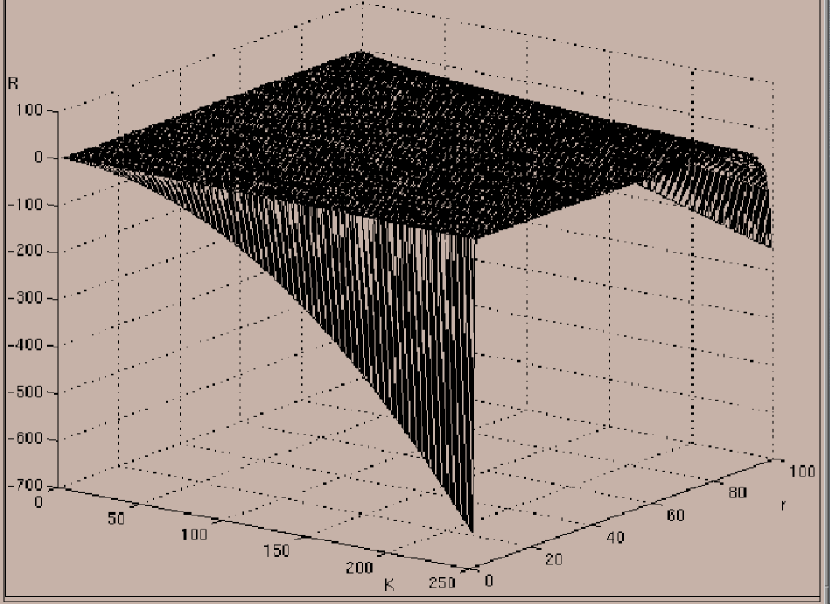
Figure 5.3: The figure shows a three-dimensional surface of the relative rate of the number of observers as function of the number of possible results $K$ for each experiment and the number $r$ of places occupied by preassigned eigenvalues (see text). The ranges of $K$ and $r$ are $2\leq K\leq 250$ and $0\leq r\leq 100$ respectively. Note the large jump towards zero for large $K$ when $r$ increases from zero.

We see from the figure that the surface, including the planar form on top of it, is inclined from positive values of $R(K,r)$, for small $K$, towards negative values for large $K$ which means that the large numbers of observers are found at large $K$ and small $r$ as we have found from Table 1. Also, as seen from the figure, the rate $R(K,r)$ decreases sharply, for small $r$, as $K$ increases, whereas this decrease is less pronounced for intermediate values of $r$ and then it strengthens again for large $r$ but less than for the small values of it as seen from the figure. When $K=1$, which means that there is only one result for any experiment we must have, for each observer, $r=n$ since there is no eigenvalue in any place of any $n$-sequence that is different from the specified ones. In this case all the sequences of all the observers are identical to each other and the probability to find in them all the $r$ specified eigenvalues, where $r=n$, is unity. In other words, the more known are the obtained results from any experiment, the larger is the probability to find in the sequences of most of them a large number of the specified eigenvalues.

We, thus, see that an important necessary aspect of the physical validation of real phenomena is that a large ensemble of related observers must be involved in the relevant experimentation. This is affected, as remarked, through the magnitude of $K$ so that the smaller is $K$ the larger is the number of observers that obtain the same results in their sequences and consequently the more valid is the tested theory. When $K=1$ which means that there is only one possible result for any experiment then the whole ensemble of observers obtains exactly the same results in their sequences. In other words, the smaller is $K$, in which case the obtained result from any experiment is less unknown, the more related are the observers of the ensemble where this relationship is demonstrated by obtaining the same results. When $K=1$ then this relationship is maximal and the whole ensemble obtains exactly the same results. Note that if they do not measure the same observables then they are totally unrelated and our former results would not be obtained even for $K=1$. As remarked, the number of possible observers increases in an asymptotic manner with the number of experiments (see Eq (5.8) and Table 1) and so all the results in this section are for large ensemble of observers.

$K=1$ corresponds, for example, to the given initial probability amplitude or particle density in the one-dimensional arrays of potential barriers or traps respectively discussed in the former chapter. It has been shown there that as the number of barriers or traps increases the corresponding initial values of the probability amplitude or particles density is preserved in passing through them. This corresponds to the results obtained here and strengthened by Table 1 that the more small is $K$, in which case the initial state is less unknown then a larger number of observers obtain similar results. When the initial state is known ($K=1$) then the whole ensemble obtains exactly the same results. Thus, we see that the new response of the system, identified here by the large probability to find in the sequences of most observers the same eigenvalues for small $K$, is possible only for large ensemble of related observers. This relationship is manifested by the fact that all the observers measure the same observables, so that the new response is obtained only as a result of it. Otherwise, this new phenomenon would not be obtained even for $K=1$. Also, as for the other examples discussed in the former chapters, this new response may be physically established by merely repeating again this collective experiment for small $K$. As remarked, the number of possible observers increases in an asymptotic manner with the number of experiments (see Eq (5.8) and Table 1). Thus, all the results in this chapter are for large ensemble of observers.

Table 5.1: The table shows the number of observers that have $r$ positions in their 100 places sequences occupied by the preassigned eigenvalues, where the numbers $K$ of possible values for each experiment are 1100, 100, 10, 5 and 2

r	Number   of	Number   of	Number   of	Number   of	Number   of
	observers for	observers for	observers for	observers for	observers for
	K=1100	K=100	K=10	K=5	K=2
$0.$	$1.2582567\cdot 10^{306}$	$3.6603234\cdot 10^{201}$	$2.6561399\cdot 10^{97}$	$1.6069380\cdot 10^{62}$	$1.0000000\cdot 10^{02}$
$2.$	$9.1968147\cdot 10^{300}$	$3.6599499\cdot 10^{199}$	$3.5349615\cdot 10^{98}$	$2.4360176\cdot 10^{64}$	$9.7020000\cdot 10^{05}$
$4.$	$7.0906332\cdot 10^{298}$	$3.4773445\cdot 10^{199}$	$4.0638965\cdot 10^{100}$	$1.4177623\cdot 10^{67}$	$9.0345024\cdot 10^{09}$
$6.$	$5.2425320\cdot 10^{296}$	$3.1683182\cdot 10^{199}$	$4.4803204\cdot 10^{102}$	$7.9128857\cdot 10^{69}$	$8.0678106\cdot 10^{13}$
$8.$	$3.7137826\cdot 10^{294}$	$2.7658535\cdot 10^{199}$	$4.7325459\cdot 10^{104}$	$4.2314156\cdot 10^{72}$	$6.9028188\cdot 10^{17}$
$10.$	$2.5182857\cdot 10^{292}$	$2.3112275\cdot 10^{199}$	$4.7851297\cdot 10^{106}$	$2.1659559\cdot 10^{75}$	$5.6534086\cdot 10^{21}$
$12.$	$1.6329854\cdot 10^{290}$	$1.8469068\cdot 10^{199}$	$4.6268069\cdot 10^{108}$	$1.0602354\cdot 10^{78}$	$4.4277496\cdot 10^{25}$
$14.$	$1.0115902\cdot 10^{288}$	$1.4099129\cdot 10^{199}$	$4.2737987\cdot 10^{110}$	$4.9579258\cdot 10^{80}$	$3.3128423\cdot 10^{29}$
$16.$	$5.9800861\cdot 10^{285}$	$1.0271175\cdot 10^{199}$	$3.7672744\cdot 10^{112}$	$2.2124744\cdot 10^{83}$	$2.3653694\cdot 10^{33}$
$18.$	$3.3697990\cdot 10^{283}$	$7.1324983\cdot 10^{198}$	$3.1654407\cdot 10^{114}$	$9.4113129\cdot 10^{85}$	$1.6098704\cdot 10^{37}$
$20.$	$1.8079384\cdot 10^{281}$	$4.7157013\cdot 10^{198}$	$2.5323525\cdot 10^{116}$	$3.8115817\cdot 10^{88}$	$1.0431960\cdot 10^{41}$
$22.$	$9.2238011\cdot 10^{278}$	$2.9648150\cdot 10^{198}$	$1.9264637\cdot 10^{118}$	$1.4679354\cdot 10^{91}$	$6.4281738\cdot 10^{44}$
$24.$	$4.4690875\cdot 10^{276}$	$1.7702375\cdot 10^{198}$	$1.3918106\cdot 10^{120}$	$5.3689737\cdot 10^{93}$	$3.7617673\cdot 10^{48}$
$26.$	$2.0536029\cdot 10^{274}$	$1.0024301\cdot 10^{198}$	$9.5364800\cdot 10^{121}$	$1.8623628\cdot 10^{96}$	$2.0877809\cdot 10^{52}$
$28.$	$8.9366846\cdot 10^{271}$	$5.3757503\cdot 10^{197}$	$6.1881159\cdot 10^{123}$	$6.1178617\cdot 10^{98}$	$1.0973376\cdot 10^{56}$
$30.$	$3.6773709\cdot 10^{269}$	$2.7259952\cdot 10^{197}$	$3.7969057\cdot 10^{125}$	$1.9003608\cdot 10^{101}$	$5.4537680\cdot 10^{59}$
$32.$	$1.4285652\cdot 10^{267}$	$1.3050066\cdot 10^{197}$	$2.1993928\cdot 10^{127}$	$5.5728080\cdot 10^{103}$	$2.5589079\cdot 10^{63}$
$34.$	$5.2302616\cdot 10^{264}$	$5.8879085\cdot 10^{196}$	$1.2007055\cdot 10^{129}$	$1.5401848\cdot 10^{106}$	$1.1315491\cdot 10^{67}$
$36.$	$1.8014464\cdot 10^{262}$	$2.4991021\cdot 10^{196}$	$6.1665865\cdot 10^{130}$	$4.0044805\cdot 10^{108}$	$4.7072442\cdot 10^{70}$
$38.$	$5.8258354\cdot 10^{259}$	$9.9596905\cdot 10^{195}$	$2.9736650\cdot 10^{132}$	$9.7759381\cdot 10^{110}$	$1.8386496\cdot 10^{74}$
$40.$	$1.7654032\cdot 10^{257}$	$3.7192600\cdot 10^{195}$	$1.3436561\cdot 10^{134}$	$2.2362458\cdot 10^{113}$	$6.7294575\cdot 10^{77}$
$42.$	$5.0018254\cdot 10^{254}$	$1.2985724\cdot 10^{195}$	$5.6765321\cdot 10^{135}$	$4.7827708\cdot 10^{115}$	$2.3028204\cdot 10^{81}$
$44.$	$1.3218922\cdot 10^{252}$	$4.2292041\cdot 10^{194}$	$2.2369741\cdot 10^{137}$	$9.5416277\cdot 10^{117}$	$7.3506026\cdot 10^{84}$
$46.$	$3.2505518\cdot 10^{249}$	$1.2815770\cdot 10^{194}$	$8.2022385\cdot 10^{138}$	$1.7711646\cdot 10^{120}$	$2.1831290\cdot 10^{88}$
$48.$	$7.4172159\cdot 10^{246}$	$3.6037407\cdot 10^{193}$	$2.7907863\cdot 10^{140}$	$3.0508311\cdot 10^{122}$	$6.0167034\cdot 10^{91}$
$50.$	$1.5659782\cdot 10^{244}$	$9.3761236\cdot 10^{192}$	$8.7858088\cdot 10^{141}$	$4.8622621\cdot 10^{124}$	$1.5342594\cdot 10^{95}$
$52.$	$3.0494930\cdot 10^{241}$	$2.2500401\cdot 10^{192}$	$2.5511386\cdot 10^{143}$	$7.1475252\cdot 10^{126}$	$3.6085781\cdot 10^{98}$
$54.$	$5.4586840\cdot 10^{238}$	$4.9633574\cdot 10^{191}$	$6.8093353\cdot 10^{144}$	$9.6580935\cdot 10^{128}$	$7.8017458\cdot 10^{101}$
$56.$	$8.9486549\cdot 10^{235}$	$1.0026985\cdot 10^{191}$	$1.6645042\cdot 10^{146}$	$1.1951891\cdot 10^{131}$	$1.5447457\cdot 10^{105}$
$58.$	$1.3380740\cdot 10^{233}$	$1.8476415\cdot 10^{190}$	$3.7112278\cdot 10^{147}$	$1.3490697\cdot 10^{133}$	$2.7898107\cdot 10^{108}$
$60.$	$1.8168898\cdot 10^{230}$	$3.0916560\cdot 10^{189}$	$7.5140909\cdot 10^{148}$	$1.3827964\cdot 10^{135}$	$4.5752895\cdot 10^{111}$

r	Number   of	Number   of	Number   of	Number   of	Number   of
	observers for	observers for	observers for	observers for	observers for
	K=1100	K=100	K=10	K=5	K=2
$62.$	$2.2293661\cdot 10^{227}$	$4.6748640\cdot 10^{188}$	$1.3748003\cdot 10^{150}$	$1.2808152\cdot 10^{137}$	$6.7805790\cdot 10^{114}$
$64$	$2.4586134\cdot 10^{224}$	$6.3533505\cdot 10^{187}$	$2.2607828\cdot 10^{151}$	$1.0662786\cdot 10^{139}$	$9.0317313\cdot 10^{117}$
$66.$	$2.4223775\cdot 10^{221}$	$7.7139956\cdot 10^{186}$	$3.3213969\cdot 10^{152}$	$7.9304473\cdot 10^{140}$	$1.0747760\cdot 10^{121}$
$68.$	$2.1179239\cdot 10^{218}$	$8.3113758\cdot 10^{185}$	$4.3301175\cdot 10^{153}$	$5.2340952\cdot 10^{142}$	$1.1349635\cdot 10^{124}$
$70.$	$1.6307895\cdot 10^{215}$	$7.8865212\cdot 10^{184}$	$4.9716164\cdot 10^{154}$	$3.0423178\cdot 10^{144}$	$1.0555160\cdot 10^{127}$
$72.$	$1.0963736\cdot 10^{212}$	$6.5338795\cdot 10^{183}$	$4.9838920\cdot 10^{155}$	$1.5439763\cdot 10^{146}$	$8.5707902\cdot 10^{129}$
$74.$	$6.3723598\cdot 10^{208}$	$4.6799137\cdot 10^{182}$	$4.3193730\cdot 10^{156}$	$6.7741960\cdot 10^{147}$	$6.0166947\cdot 10^{132}$
$76.$	$3.1656008\cdot 10^{205}$	$2.8649609\cdot 10^{181}$	$3.1995356\cdot 10^{157}$	$2.5403235\cdot 10^{149}$	$3.6100168\cdot 10^{135}$
$78.$	$1.3262069\cdot 10^{202}$	$1.4791044\cdot 10^{180}$	$1.9987222\cdot 10^{158}$	$8.0337731\cdot 10^{150}$	$1.8266685\cdot 10^{138}$
$80.$	$4.6117440\cdot 10^{198}$	$6.3383721\cdot 10^{178}$	$1.0363745\cdot 10^{159}$	$2.1088654\cdot 10^{152}$	$7.6720078\cdot 10^{140}$
$82.$	$1.3058579\cdot 10^{195}$	$2.2117368\cdot 10^{177}$	$4.3758034\cdot 10^{159}$	$4.5076999\cdot 10^{153}$	$2.6238267\cdot 10^{143}$
$84.$	$2.9408267\cdot 10^{191}$	$6.1380718\cdot 10^{175}$	$1.4694056\cdot 10^{160}$	$7.6630898\cdot 10^{154}$	$7.1368085\cdot 10^{145}$
$86.$	$5.1132066\cdot 10^{187}$	$1.3151669\cdot 10^{174}$	$3.8095700\cdot 10^{160}$	$1.0057805\cdot 10^{156}$	$1.4987298\cdot 10^{148}$
$88.$	$6.6042355\cdot 10^{183}$	$2.0933174\cdot 10^{172}$	$7.3369497\cdot 10^{160}$	$9.8063602\cdot 10^{156}$	$2.3380185\cdot 10^{150}$
$90.$	$6.0147815\cdot 10^{179}$	$2.3494022\cdot 10^{170}$	$9.9637588\cdot 10^{160}$	$6.7418726\cdot 10^{157}$	$2.5718203\cdot 10^{152}$
$92.$	$3.5855598\cdot 10^{175}$	$1.7259153\cdot 10^{168}$	$8.8566745\cdot 10^{160}$	$3.0338427\cdot 10^{158}$	$1.8517106\cdot 10^{154}$
$94.$	$1.2468404\cdot 10^{171}$	$7.3960252\cdot 10^{165}$	$4.5923497\cdot 10^{160}$	$7.9638371\cdot 10^{158}$	$7.7771846\cdot 10^{155}$
$96.$	$2.0646454\cdot 10^{166}$	$1.5092389\cdot 10^{163}$	$1.1339135\cdot 10^{160}$	$9.9547963\cdot 10^{158}$	$1.5554369\cdot 10^{157}$
$98.$	$1.0256551\cdot 10^{161}$	$9.2392953\cdot 10^{159}$	$8.3993594\cdot 10^{158}$	$3.7330486\cdot 10^{158}$	$9.3326215\cdot 10^{157}$

5.4 The classical effect of an ensemble of observers

We discuss now the same system used in [76] for demonstrating the effect of observers upon the experimental results. The discussion in [76] is generalized to include the large ensemble of related observers so we assume that we have $N$ thermodynamical systems, of the kind discussed in [76], that is, a hollow cylinder that contains $n$ particles, not all of the same species, among four pistons as shown in Figure 5.4. The pistons $A$ and $\grave{A}$ are fixed while $B$ and $\grave{B}$ may move along the cylinder. Also the pistons $\grave{A}$ and $B$ do not allow passage of particles through them, whereas $A$ and $\grave{B}$ are permeable so that each permits some kind of particles to move through it where those that are allowed to pass through $A$ are not allowed through $\grave{B}$ and vice versa. The pistons $B$ and $\grave{B}$ move in such a way that the distances $B\grave{B}$ and $A\grave{A}$ are always equal as seen in Figure 5.4. These distances are measured using the $x$ axis which is assumed to be upward along the cylinder.

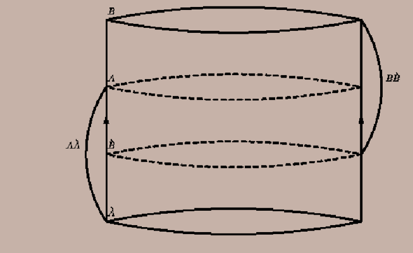
Figure 5.4: The cylinder with the four pistons. The pistons $A$ and $\grave{A}$ are fixed and $B$ and $\grave{B}$ may move along the cylinder. Also the piston $A$ is permeable to the molecule inside the interval $(x_{1},x_{2})$ and $\grave{B}$ to those outside it.

We wish to test the validity of the connection (suggested in [76]) between the two variables $x$ and $f$, where the latter denotes the property that if any of the $n$ particles is found in some preassigned interval $(x_{1},x_{2})$ then we assign to $f$ the value of $+1$ otherwise $f$ assumes the value of $-1$. That is, the relevant proposed connection between $x$ and $f$ is [76]

$$f(x)=\left\{\begin{array}[]{ll}+1&{\rm for\leavevmode\nobreak\ }x_{2}\geq x\geq x_{1}\\ -1&{\rm for\ x\ outside\leavevmode\nobreak\ }(x_{1},x_{2})\end{array}\right.$$ (5.44)

We assume that the piston $A$ is permeable only to the particles inside the interval $(x_{1},x_{2})$ and $\grave{B}$ only to those outside it. We denote by $w_{1}$ the initial probability that any randomly selected particle is found to be in the interval $(x_{1},x_{2})$ and by $w_{2}$ that it is outside it. At first the pistons $B$ and $\grave{B}$ were at the positions of $A$ and $\grave{A}$ respectively and all the $n$ particles were in the one space between. Now, we wish to test the assumed relation from Eq (5.44) by performing, reversibly and with no external force, a complete cycle of first moving up the pistons $B\grave{B}$ and then retracing them back to their initial places so that the only assumed relation between the particles and their positions along the axis $x$ is that from Eq (5.44). Thus, we first move, without doing work, the pistons $B$ and $\grave{B}$ so that, as remarked, the volume enclosed between them equals that between $A\grave{A}$ and we obtain two separate equal volumes, each of which equals to the initial one. Now, since $A$ is permeable to the particles in the interval $(x_{1},x_{2})$ and $\grave{B}$ to the rest the result is that the upper volume $B\grave{B}$ contains only the particles from the predetermined interval $(x_{1},x_{2})$ and the lower $A\grave{A}$ only the others.

We want now to retrace our former steps and move, again without doing work, the pistons $B$ and $\grave{B}$ to the places of $A$ and $\grave{A}$ so as to have, as before, the same initial volume and thus to complete one cycle. We must take into account, however, that during the upward motion some particles that were inside (outside) the interval $(x_{1},x_{2})$ may come out of (into) it due to thermal or other kind of fluctuation so that these particles change from the kind that may pass through the piston $A$ ($\grave{B}$) into the kind that is not allowed to do that. Thus, the last step of retracing the pistons $B$, $\grave{B}$ into their former initial positions at the pistons $A$, $\grave{A}$ respectively can not be performed without doing work since the molecules that have come out of (into) the interval $(x_{1},x_{2})$ are not permitted now to pass through $A$ ($\grave{B}$). That is, the former process of expanding the volume is not reversible as described because we have to exert force on these molecules to move them back into (out of) the interval $(x_{1},x_{2})$ so that they can pass through $A$ ($\grave{B}$). Thus, the relation (5.44) is not valid any more since it does not take into account the external force just described.

We may express this in a quantitative manner by noting that there is now [76] a decrease of entropy per molecule after the first step of moving up the pistons. This may be calculated by taking account of the fact that now the probabilities to find any randomly selected molecule out of (in) the preassigned interval $(x_{1},x_{2})$ are different from the initial values $w_{2}$ and $w_{1}$ before moving up the pistons. Thus, suppose that during the first stage of expanding the initial volume of the cylinder $n_{o}$ molecules, from the total number $n$, have come out of the remarked interval and $n_{i}$ from outside have entered so that the probability to find now any randomly selected molecule out of it is $(w_{2}+\frac{(n_{o}-n_{i})}{n})$ and that to find it in is $(w_{1}+\frac{(n_{i}-n_{o})}{n})$. Thus, the initial entropy per molecule, denoted by $s_{i}$, before moving up the pistons is [76]

$$s_{i}=-k(w_{1}\ln w_{1}+w_{2}\ln w_{2}),$$ (5.45)

and after moving-up the pistons the corresponding entropy per molecule, denoted by $s_{m}$, is

$$s_{m}=-k((w_{1}+\frac{(n_{i}-n_{o})}{n})\ln(w_{1}+\frac{(n_{i}-n_{o})}{n})+$$ (5.46)

$$+(w_{2}+\frac{(n_{o}-n_{i})}{n})\ln(w_{2}+\frac{(n_{o}-n_{i})}{n}))$$

The difference in the entropy per molecule between the two situations from Eqs (5.45)- (5.46) is

$$s=-(s_{m}-s_{i})=-(kw_{1}(\ln(w_{1}+\frac{(n_{i}-n_{o})}{n})-\ln w_{1})+kw_{2}(\ln(w_{2}+$$

$$+\frac{(n_{o}-n_{i})}{n})-\ln w_{2})+k\frac{(n_{o}-n_{i})}{n}(\ln(w_{2}+\frac{(n_{o}-n_{i})}{n})-$$ (5.47)

$$-\ln(w_{1}+\frac{(n_{i}-n_{o})}{n})))=-(kw_{1}\ln(1+\frac{(n_{i}-n_{o})}{w_{1}n})+kw_{2}\ln(1+\frac{(n_{o}-n_{i})}{w_{2}n})+$$

$$+k\frac{(n_{o}-n_{i})}{n}\ln(\frac{w_{2}+\frac{(n_{o}-n_{i})}{n}}{w_{1}+\frac{(n_{i}-n_{o})}{n}}))=-(k(w_{1}(1+\frac{(n_{i}-n_{o})}{w_{1}n})\ln(1+\frac{(n_{i}-n_{o})}{w_{1}n})+$$

$$+w_{2}(1+\frac{(n_{o}-n_{i})}{w_{2}n})\ln(1+\frac{(n_{o}-n_{i})}{w_{2}n})+\frac{(n_{o}-n_{i})}{n}\ln(\frac{w_{2}}{w_{1}})))$$

Eliminating $w_{2}$ through use of the relation $w_{1}+w_{2}=1$ one may write the last equation as

$$s=-(s_{m}-s_{i})=-k(w_{1}(1-\frac{(n_{o}-n_{i})}{nw_{1}})\ln(1-\frac{(n_{o}-n_{i})}{nw_{1}})+$$ (5.48)

$$+(1-w_{1})(1+\frac{(n_{o}-n_{i})}{n(1-w_{1})})\ln(1+\frac{(n_{o}-n_{i})}{n(1-w_{1})})+\frac{(n_{o}-n_{i})}{n}\ln(\frac{(1-w_{1})}{w_{1}}))$$

If $n_{o}=n_{i}$, the entropy difference from Eqs (5.48) is obviously zero which results in the validation of the relation (5.44) after returning the pistons back to their initial places as remarked. When $n_{o}\neq n_{i}$ the expression (5.44) can not be validated by retracing, without doing work, the volume back to its initial value since now the molecules that come out of the interval $(x_{1},x_{2})$ and those that have entered it prevent this reversible motion which is necessary for its validation. Thus, a new expression, instead of the invalid one from Eq (5.44), that takes account of these molecules must be adopted as in [76]. But before writing this expression we remark that the probability $w_{1}$ must be proportional to the length of the remarked interval $x_{2}-x_{1}$, so that a small or large value for one indicates a corresponding value for the other. Thus, we may define a probability distribution for $w_{1}$ in terms of the variable $x$ and assume a normal distribution [80] so that we may write for the density function of $w_{1}(x)$ $f_{w_{1}}(x)=\frac{\exp(-\frac{(x-\mu)^{2}}{2\sigma^{2}})}{\sqrt{2\pi}\sigma}$, where $\mu$ is the mean value of $x$ and $\sigma$ is the standard deviation. To simplify the following calculation we assume a standard normal distribution [80] $z=\frac{(x-\mu)}{\sigma}$ for which $\mu=0$ and $\sigma=1$. Thus, the density function $f_{w_{1}}(x)$ may be written as $f_{w_{1}}(z)=\frac{\exp(-\frac{(z)^{2}}{2})}{\sqrt{2\pi}}$ and the probability $w_{1}(x)$ to find any randomly selected molecule in the interval $(-x,x)$, where now this interval is symmetrically located around the origin $x=0$, is [80]

$$w_{1}(x)=\int_{-x}^{x}f_{w_{1}}(z)dz=\frac{1}{\sqrt{2\pi}}\int_{-x}^{x}dze^{-\frac{z^{2}}{2}}=erf(\frac{x}{\sqrt{2}})$$ (5.49)

$erf(x)$ is the error function defined as $erf(x)=\frac{2}{\sqrt{\pi}}\int_{0}^{x}e^{-u^{2}}du$. Note that $erf(0)=0$, $erf(\infty)=1$, and $erf(-x)=-erf(x)$ so that this function is appropriate for a representation of the probability $w_{1}(x)$. Substituting from Eq (5.49) into Eq (5.48) we obtain

$$s=-(s_{m}-s_{i})=-k(erf(\frac{x}{\sqrt{2}})(1-\frac{(n_{o}-n_{i})}{n\cdot erf(\frac{x}{\sqrt{2}})})\ln(1-\frac{(n_{o}-n_{i})}{n\cdot erf(\frac{x}{\sqrt{2}})})+$$

$$+(1-erf(\frac{x}{\sqrt{2}}))(1+\frac{(n_{o}-n_{i})}{n(1-erf(\frac{x}{\sqrt{2}}))})\ln(1+\frac{(n_{o}-n_{i})}{n(1-erf(\frac{x}{\sqrt{2}}))})+$$ (5.50)

$$+\frac{(n_{o}-n_{i})}{n}\ln(\frac{(1-erf(\frac{x}{\sqrt{2}}))}{erf(\frac{x}{\sqrt{2}})}))$$

Note that in order to have no negative expression under the $ln$ sign, especially for the following numerical simulations, we take the absolute values of these expressions which does not change the real calculated results. The right hand side of Eq (5.50), which yields the entropy decrease per molecule, must be multiplied by the number $n$ of molecules in the cylinder in order to obtain the total decrease of entropy after moving up the pistons. Figure 5.5 shows a three-dimensional representation of the entropy $s$ per molecule from the last equation as function of $\frac{n_{i}}{n}$ and $\frac{n_{o}}{n}$.

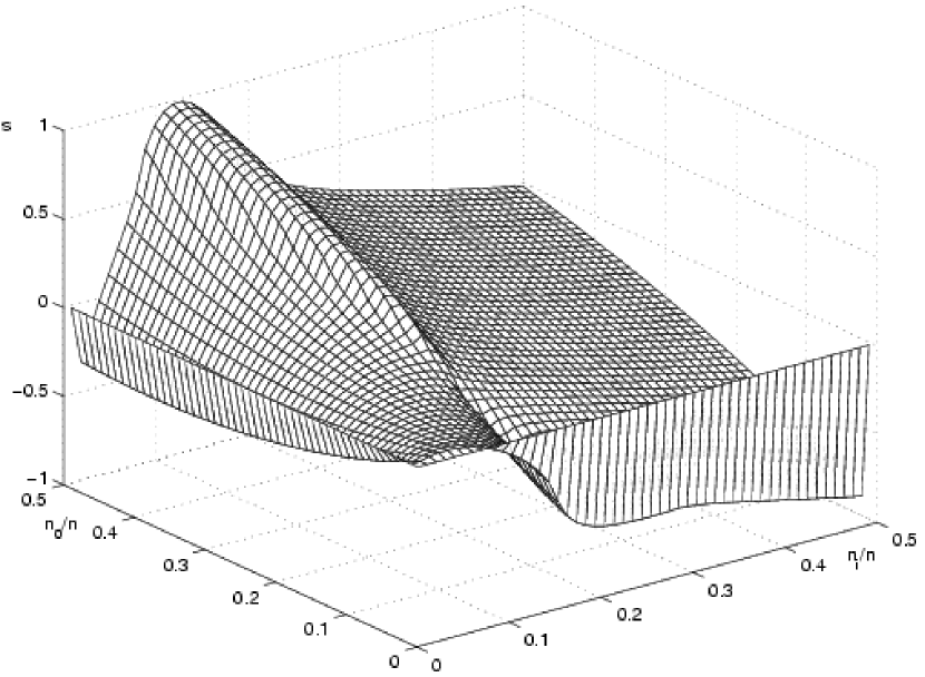
Figure 5.5: The figure shows a three-dimensional surface of the entropy per molecule $s$ as function of $\frac{n_{o}}{n}$ and $\frac{n_{i}}{n}$. Both ranges of $\frac{n_{o}}{n}$ and $\frac{n_{i}}{n}$ are $(0.005,0.5)$ since it is unexpected that in a reversible motion more than half of the total molecules will leave or enter the given interval $(x_{1},x_{2})$. Note that for large $\frac{n_{o}}{n}$ ($\frac{n_{i}}{n}$) and small $\frac{n_{i}}{n}$ ($\frac{n_{o}}{n}$) $s$ tends to $+1$ $(-1)$.

The relevant range of $w_{1}=erf(\frac{x}{\sqrt{2}})$ must begin from the minimum value of $\frac{n_{0}}{n}$ since $w_{1}$ can not be smaller than $\frac{n_{0}}{n}$. The ranges of both $\frac{n_{i}}{n}$ and $\frac{n_{o}}{n}$ are $0.005\leq\frac{n_{i}}{n},\frac{n_{o}}{n}\leq 0.5$ because in the reversible motion discussed here it is unexpected that more than half of the total particles will enter or leave the interval $(x_{1},x_{2})$. For large values of $\frac{n_{0}}{n}$ ($\frac{n_{i}}{n}$) and comparatively small values of $\frac{n_{i}}{n}$ ($\frac{n_{o}}{n}$) the entopy differences tend to $+1$ ($-1$) and when both $\frac{n_{0}}{n}$ and $\frac{n_{i}}{n}$ are large $s$ tends to zero from negative values.

The remarked problem of moving back the pistons, without doing work, to their original volume has been solved in [76] by taking into account Eq (5.44) which assign to $f(x)$ the value of $+1$ when the relevant molecule was in the interval $(x_{1},x_{2})$ and $-1$ otherwise. That is, after the first step of doubling the initial volume the cylinder includes now, except for the particles that remain inside (outside) the noted interval and characterized by $f(x)=1$ ($f(x)=-1$), also those that were in (outside) it and were denoted by these values. All these particles that were in (out of) the interval $(x_{1},x_{2})$ continue, for the short time interval between moving the pistons up and down, to be denoted by $f(x)=1$ ($f(x)=-1$). Thus, as noted in [76], for the last step of retracing to the original volume, without doing work, one has only to replace the pistons $A$ by $A^{*}$ that is permeable not with respect to the molecules in the interval $(x_{1},x_{2})$ but to those that their $f(x)$ is $+1$. Correspondingly, the piston $\grave{B}$ is replaced by $\grave{B}^{*}$ that is permeable to those that their $f(x)$ has the value of $-1$. Thus, the external intervention in this case is changed in [76] from Eq (5.44) to

$$f(x)=\left\{\begin{array}[]{ll}+1&{\rm for\ x\ that\ is\ or\ was\ in\leavevmode\nobreak\ }x_{2}\geq x\geq x_{1}\\ -1&{\rm for\ x\ that\ is\ or\ was\ outside\leavevmode\nobreak\ }(x_{1},x_{2})\end{array}\right.$$ (5.51)

In such a way one is able to perform a complete cycle of first expanding the volume with the original permeable pistons $A$ and $\grave{B}$ and then retrace this step reversibly with the pistons $A^{*}$ and $\grave{B}^{*}$ instead of $A$ and $\grave{B}$ as remarked. Thus, all the possible motions of the molecules, including their coming out of or into the given interval $(x_{1},x_{2})$ are accounted for by Eq (5.51) which results in its validation as remarked (see the discussion after Eq (5.44)).

Now, if we take into account the possible Feynman paths [30] through which the system may evolute during the remarked complete cycle then such paths may be characterized also by those that conform either to Eq (5.44) or to (5.51). That is, the Feynman paths that may result in a decrease of the entropy are those in accordance with (5.44) and those that do not result with such a change correspond to (5.51). Thus, using (5.51) is the same as passing along the specific path that preserve the entropy and rejecting those that change it (that conform to (5.44)). All one have to do is to “realize” the correct path, in the sense of [11], which is done in accordance with the former section by having a large number of observers each moving his respective piston up and down in the described manner. We calculate the correlation among the $N$ separate systems by assuming that all begin with the original pistons $A$, $\grave{A}$, $B$ and $\grave{B}$ and finding the number of them that after completing one cycle are found with the pistons $A$, $A^{*}$, $B$ and $\grave{B}^{*}$ which denote that the expression (5.44) is not valid for them. When, after expanding the initial volumes of the $N$ cylinders we find, for some of them, that no molecule from the interval $(x_{1},x_{2})$ has come out of it and no one from outside has entered then they end, after returning the volume to its initial state, with the same pistons they begin with and in such a case the expression (5.44) is obviously valid for them. But suppose that for other observers $n_{o_{j}}$ molecules come out of the interval $(x_{1},x_{2})$ and $n_{i_{j}}$ have entered where $n_{o_{j}}\neq n_{i_{j}}$. In such case the total decrease of entropy, after moving-up the pistons, using Eq (5.50) and assuming that the total number of molecules $n$ are the same for all the ensemble members, is

$$s_{total}=-k\sum_{j=1}^{j=N}n(w_{1_{j}}\ln(1+\frac{(n_{i_{j}}-n_{o_{j}})}{w_{1_{j}}n})+w_{2_{j}}\ln(1+\frac{(n_{o_{j}}-n_{i_{j}})}{w_{2_{j}}n})+$$

$$+\frac{(n_{o_{j}}-n_{i_{j}})}{n}\ln(\frac{w_{2_{j}}+\frac{(n_{o_{j}}-n_{i_{j}})}{n}}{w_{1_{j}}+\frac{(n_{i_{j}}-n_{o_{j}})}{n}})=-k\sum_{j=1}^{j=N}n(erf(\frac{x_{j}}{\sqrt{2}})(1-$$ (5.52)

$$-\frac{(n_{o_{j}}-n_{i_{j}})}{n\cdot erf(\frac{x_{j}}{\sqrt{2}})})\ln(1-\frac{(n_{o_{j}}-n_{i_{j}})}{n\cdot erf(\frac{x_{j}}{\sqrt{2}})})+(1-erf(\frac{x_{j}}{\sqrt{2}}))(1+\frac{(n_{o_{j}}-n_{i_{j}})}{n(1-erf(\frac{x_{j}}{\sqrt{2}}))})\cdot$$

$$\cdot\ln(1+\frac{(n_{o_{j}}-n_{i_{j}})}{n(1-erf(\frac{x_{j}}{\sqrt{2}}))})+\frac{(n_{o_{j}}-n_{i_{j}})}{n}\ln(\frac{(1-erf(\frac{x_{j}}{\sqrt{2}}))}{erf(\frac{x_{j}}{\sqrt{2}})}))$$

We, now, show that when the $N$ observers are related to each other in the sense that all the $N$ experiments of moving the pistons up and down are prepared in such a way that no two observers share the same values of $\frac{n_{o_{j}}}{n}$, $\frac{n_{i_{j}}}{n}$ and $x_{j}$ then the larger is $N$ the more probable is that the majority of them obtain negative entropy difference. If, on the other hand, they are not related in this manner so that some observers may have the same $\frac{n_{o_{j}}}{n}$, $\frac{n_{i_{j}}}{n}$ and $x_{j}$ then the mentioned probability will not be obtained even for large $N$. We first note that since for $x\geq 3$ $erf(x)$ is approximately the same as for $x=\infty$, we may assume a range of $(0,3)$ from which we take the values for the preassigned interval $(-x,x)$. Thus, we subdivide the interval $(-3,3)$ into $N$ subintervals, where $N$ is the number of observers, so that each has his respective interval $(-x_{j},x_{j})$ where $x_{j}$ is the corresponding real number from the range $0\leq x_{j}\leq 3$. We note, as remarked after Eq (5.50), that each probability $w_{i_{j}}$ for any observer $O_{j}\ \ (j=1,2,\ldots,N)$ must begin from the minimum value of $\frac{n_{o_{j}}}{n}$ and assume (see the discussion after Eq (5.50)) that both $\frac{n_{i_{j}}}{n}$ and $\frac{n_{o_{j}}}{n}$ are in the range $0.005\leq\frac{n_{o_{j}}}{n},\frac{n_{i_{j}}}{n}\leq 0.5$. We assign to each observer that obtains negative entropy difference after moving-up the pistons the value of $+1$ (this has nothing to do with the $+1$ or $-1$ in Eqs (5.44) and (5.51)) and 0 otherwise.

We assume that $N_{c}$ observers, of the total $N$, lift up their respective pistons and we calculate the fraction

$$f_{N_{c}}(N)=\frac{1}{N}\sum_{i=1}^{i=N_{c}}g_{i}(N),$$ (5.53)

where $g_{i}(N)=1$ if the result of any of these experiments yields a negative value for the entropy difference and $g_{i}(N)=0$ otherwise. It is shown, as remarked, that as $N$ grows this fraction increases and with it the probability that most of them obtain negative entropy differences in which case they end, according to the rules of the experiment (see the discussion after Eq (5.51)), with the replaced pistons $A^{*}$ and $\grave{B}^{*}$ in place of the original ones $A$ and $\grave{B}$ so that the relation (5.51) is established for most of them. Figure 5.6 shows the remarked fraction $f_{N_{c}}(N)$ as a function of the $N$ observers and we see that $f_{N_{c}}(N)$ grows as $N$ increases. That is, the presence of a large number of observers resulted with the outcome that a large number of experiments end with a negative entropy difference. The same result has been obtained in the former section for the effect of a large ensemble of related observers that perform experiments where any result obtained by any one is valid for all the others (see the discussion after Eq (5.5) and also Figure 5.2).

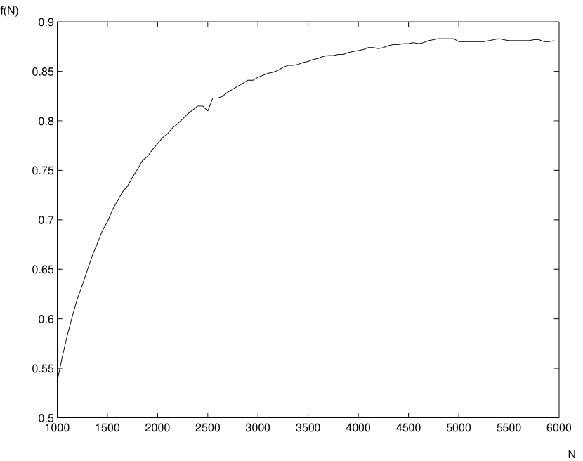
Figure 5.6: The curve shows the result of performing 1000 different experiments of lifting up the pistons as a function of the number of observers $N$ (that only 1000 of them perform the experiments). Note that no two of the 1000 experiments are identical and that each is deliberately performed for different values of the intervals $(-x_{j},x_{j})$, $\frac{n_{o_{j}}}{n}$ and $\frac{n_{i_{j}}}{n}$ where $x_{j}=6\cdot\frac{n_{o_{j}}}{n}$. Note that as $N$ grows the number of experiments that end in negative entropy decrease increases.

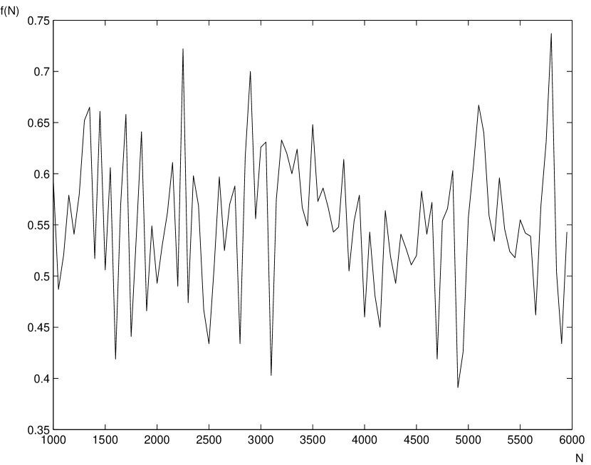
Figure 5.7: The stochastic curve shown is drawn for exactly the same conditions as those of Figure 5.6, except that the values of $(-x_{j},x_{j})$, $\frac{n_{o_{j}}}{n}$ and $\frac{n_{i_{j}}}{n}$ are chosen randomly. That is, the curve shows the results of 1000 experiments as a function of the number of observers $N$. Note that some of these experiments may be identical due to the random conditions under which they are performed. Also, as seen from the graph there is no discernable increase or decrease of $f(N)$ with $N$ (compare with Figure 5.6).

The results of Figure 5.6 are obtained by choosing for $\frac{n_{o}}{n}$ and $\frac{n_{i}}{n}$, that are both confined in the range $(0.005,05)$, the values of $\frac{n_{o}(j)}{n}=0.005+\frac{(0.5-0.005)j}{49}$, and $\frac{n_{i}(l,k)}{n}=0.005+\frac{(0.5-0.005)l}{(20+k)}$, where $0\leq j\leq 49$, $0\leq l\leq 120$ and $0\leq k\leq 100$. Note that the common total interval $(0.005,05)$ of $\frac{n_{o}}{n}$ and $\frac{n_{i}}{n}$ has been subdivided differently for them. That is, for $\frac{n_{o}}{n}$ the division is to 50 equally spaced values and for $\frac{n_{i}}{n}$ it is to 121. That is, the maximum possible number of observers is $N_{max}=121\cdot 50=6050$ and we assume, for the numerical analysis, that 1000 of them participate in the experiments so that $N_{c}=1000$. Thus, all the observers are related in the sense that each has its specific $\frac{n_{o_{j}}}{n}$ and $\frac{n_{i_{j}}}{n}$. If, on the other hand, this kind of connection is absent as when assigning randomly to any observer $O_{j}\ \ (j=1,2,\ldots,N)$ an interval $(-x_{j},x_{j})$ and also $\frac{n_{o_{j}}}{n}$, $\frac{n_{i_{j}}}{n}$ from $(0.005,0.5)$ we obtain a stochastic result for $f(N)$ that implies no increase (and no decrease) of the number of observers that get negative entropy difference. This is seen clearly from the sawtooth form of the curve of Figure 5.7 which is drawn under exactly the same conditions as those of Figure 5.6 except that the values of $(-x_{j},x_{j})$, $\frac{n_{o_{j}}}{n}$ and $\frac{n_{i_{j}}}{n}$ are randomly assigned to the observers.

We, thus, see that when the observers are related among them the probability to find any one of them (that begin with the pistons $A$, $\grave{A}$, $B$ and $\grave{B}$) ending with $A$, $A^{*}$, $B$ and $\grave{B}^{*}$ is large so that, as remarked, the relation (5.51) is physically established the larger is the number $N$ of related observers. We note that for Figures 5.6 - 5.7 we have expressed the values of $x_{j}$ from the interval $(-x_{j},x_{j})$ in terms of $\frac{n_{o_{j}}}{n}$ as $x_{j}=6\cdot\frac{n_{o_{j}}}{n}$. In such a way each observer $O_{j}(j=1,2,\ldots N)$ that has been assigned a specific value of $\frac{n_{o_{j}}}{n}$ from the remarked range $0.005\leq\frac{n_{o_{j}}}{n}\leq 0.5$ is automatically assigned a corresponding value from the range $0.03\leq x_{j}\leq 3$. Thus, the maximum value of $x_{j}$ is in accordance with the discussion after Eq (5.52).

We note that the same results may be obtained by using other methods and terminology. Thus, it is shown [81] that the “localization” (in the sense of smaller dispersion) for the state $|\phi\!>$ is greater the smaller is the entropy which results when the rate of “effective interaction with the environment” [81] increases. Localization is another phrase for what we call here “realizing or preserving a specific state” and the interaction with the environment is equivalent to performing experiment [13, 26, 82, 83], so that as the rate of performing experiment grows the more realized and localized is the state one begins with or the path of states along which one proceeds.

We see, therefore, that the classical thermodynamical system discussed here obeys also the same development we have encountered in the former chapters regarding the evolution of new phenomena (and their theories). That is, the establishment of the assumed physical connection from Eq (5.51) between the variables $f$ and $x$ proceeds by first trying the form (5.44) but it soon becomes clear, by testing it through experiments, that there is a gap between it and the experimental results with regard to the molecules that come out of (into) the preassigned interval $(x_{1},x_{2})$. Thus, in order to conform to the experimental findings one have to replace the weak theory of (5.44) by the new expression from Eq (5.51) which takes into account these molecules. The new theory entails a corresponding change in the experimental set-up that is supposed to validate it. That is, the replacement of the pistons $A$ and $\grave{B}$ by $A^{*}$ and $\grave{B}^{*}$ in the second stage of reversing back, without doing work, to the former volume. The important step that assigns to the relation (5.51) a physical aspect is obtained, as remarked, when a large number of related observers perform the relevant experiments with their cylinders and obtain similar results (see Figure 5.6). Unrelated ensemble of observers, no matter how large it is, does not obtain the sought-for physical validation of the new relation from Eq (5.51) as seen clearly from Figure 5.7.

The new response (new phenomenon) in this case is clearly illustrated in Figure 5.6 which shows that the larger is the ensemble of related observers the larger is the number of them that obtains negative entropy difference. The last result indicates, as remarked, that the system responds in a new and different manner from the expected response of the old theory (5.44). Thus, the failure of the relation (5.44) to cope with the experimental findings necessitates a new relation (5.51) which has been shown to be more validated the larger is the number of related observers. In other words, as seen in all our work thus far, the large number of related observers that perform the experiments not only give rise to this new response of finding most of them with a negative entropy difference but also physically establish this outcome.

Chapter 6 EPILOG

We have discussed, using examples that range from quantum and classical field events, through Internet webmastering to classical thermodynamics, the possible evolutions of real phenomena especially at the initial stage of which when they are first encountered and their nature is not clear. The physical character of these new-encountered phenomena is established only after initially trying to explain them by suitable theories that must stand the tests of experiments which are prepared to reconstruct these phenomena under various conditions. We have shown that the larger is the number of repetitions of the relevant experiments the more valid and real these new phenomena will be assuming that most of these experiments result in establishing them. We have also shown that the process of validating and establishing the physical aspect of real phenomena may be explained as if it results from experimenting upon a physical system in an uninterrupted manner, that is, to the Zeno effect. Under this condition of dense measurement the known response of the system, in the absence of this dense experimentation, changes entirely to a new, and even unexpected, one as shown with respect to the one-dimensional systems discussed in Chapter 4. This new behaviour of the system may always be repeated and reconstructed any number of times by performing this dense measurement again. That is, it may be physically established under this kind of experimentation.

We note that at the initial stage before the new response becomes physically established by dense measurement the system’s response and evolution under a measurement (not dense) may assumes any of a large number of possible different ones. Thus, the corresponding initial theory, before it becomes physically established through the remarked experiments, may be described as having a possible dependence upon an extra variable that takes account of the large possible evolutions, allowed at this initial time, for the relevant system. In Section 2.2 we have discussed (see Appendix $A_{2}$) the generalization of quantum mechanics through the Flesia-Piron extension of the Lax-Phillips theory in which the extra time variable $t$ has been explicitly introduced besides the laboratory time parameter $\tau$. We do so also in [9] by using the stochatic quantization theory of Parisi-Wu [46, 42] where the introduced extra variable $s$ takes account of an assumed stochastic process (in this variable) that allows, as all stochastic processes do, a large different possible behaviours of the system. The equilibrium configuration is obtained [46, 42] when this variable is eliminated through equating all its different values to each other and taking to infinity. This equating of all the possible $s$ values to each other introduces an element of repetitions of the same process through which the system is stabilized and brought to its physical equilibrium configuration. We have shown this in [9] for the examples of the Internet websites of the harmonic oscillator and those of the energy shift (Lamb shift) [64, 65]. The same result was obtained in [51] for the general Internet websites without specifying any particular one. For this discussion of the Internet statistics we use the formalism of Ursell-Mayer [50, 49] in which an extra variable has been introduced. We note that this additional variable is not of the same kind as that of the SQ extra variable [42, 46] discussed in [9]. This extra variable is implicitly referred to in Section 2.1 (see Appendix $A_{1}$) when we discuss the bubble and open-oyster processes. This is because we do not sum there the Feynman diagrams of these processes to all orders, as usually done in quantum field theory, but their $n$ time repetitions where $n\to\infty$. The resulted double sum has the same effect as introducing an extra variable and summing over all its possible values.

The same effect of establishing the physical character of the new phenomena and their theories is obtained through a collective experiment performed by a large number of related observers. It results, as remarked, in “realizing” [11, 12] the relevant Feynman path of states, that represents the tested phenomenon, for all the observers as if each has performed dense measurement along it. This is because, although each one is restricted to do only his specific experiment, nevertheless, since all the observers have similar systems the specific results obtained by any one may, under the same conditions, be obtained by any other. Thus, the experimental results obtained by any one are valid for all the others.

This outcome of the ensemble of related systems was corroborated also upon comparing the mechanism just described to the procedure of numerical simulations. This has been shown in [9] with regard to a large ensemble of related computers and in [51] in connection to a corresponding large cluster of mutually linked websites and in both cases the same outcome was obtained. Thus, the relationship among the ensemble of related computers is strengthened by seeing to it that the actions $S$ of all or most of the path integrals that represent them contain the same expression [9] that characterizes the involved interaction simulated by them such as that of the harmonic oscillator or of the Lamb shift [9]. In such a way all the related computers may be brought, as shown in [9], to the situation in which all of them have the same common sites and, therefore, their correlation is maximal. These effects of the ensemble of related systems were demonstrated also in [51] by using the cluster formalism of Ursell [49] and Mayer [50] where a large ensemble of connected computers (users) may aquire a very large additional amount of connectivity [67] among them by adding only a small number of connecting website links. The correspondence between computer simulations and real experimentation is sharply reflected at the last stage of running the written code on the computer screen, especially if it simulates some physical process which is governed, as most physical processes are, by a differential equation. This is because the numerical solutions of these equations are obtained by updating them a large number of times. Moreover, the larger is the number of these iterations the larger is the number of samples and the better is the resulting statistics. All the remarked effects of the ensemble of related observers have been demonstrated even more pronouncedly for the classical thermodynamical system of cylinder and pistons discussed in Chapter 5. We have also shown that when the observers are not related to each other then this “realization” of the specific evolution will not be obtained.

All these processes correspond to the Zeno effect [2, 10, 11, 12, 13, 14] by which an equilibrium physical configuration is obtained as a consequence of these repetitions. We have shown that it is effective not only for repeating the same experiment on the same system a large number of times in a finite time but also when a large number of observers, all confined in a finite region of space, perform similar experiments as shown by the various examples discussed here and in [17, 18, 20, 23]. The last effect is the space Zeno effect, described in details in Chapters 4-5, which has been demonstrated for both quantum and classical regimes and which, actually, stands in the basis of the influence of the ensemble of related observers compared to that of the single observer or of the unrelated ensemble of them. The discussion in Chapter 4 of the quantum and classical systems of the respective one-dimensional arrays of potential barriers and traps confined to finite spatial section demonstrates in a clear fashion the unique nature of space dense measurement. The responses of both systems to increasing the number of barriers or traps in the finite section, which is equivalent to increasing the rate of experiments, is not only new but also contrary to what one may expect as explained in Chapter 4 (see Appendices $C_{2}$, $C_{3}$ and $C_{4}$). That is, the dense measurement process has produced, as remarked, a new phenomenon that has not been encountered before. Moreover, this new phenomenon is not a temporary one but may be repeated and reconstructed any times we wish by performing again these dense measurements. In other words, this kind of experimentation not only gives rise to new phenomena but also may physically establish and validate them. We remark that the appearance of physical phenomena due to only repeating the same experiment a large number of times has been experimentally demonstrated [10] using various methods and techniques.

We note that this Zeno effect by which one Feynman path of states, from a large number of possible ones, is “realized” whereas the probability for the other paths tends to zero satisfies the consistency conditions of the histories formalism of Gell-Mann-Hartle and Griffiths [27, 28, 29]. That is, only one evolution is effected in the final stage and not a superposition of them (see Appendix $A_{2}$).

Chapter 7 APPENDICES

7.1 APPENDIX $A$:

ABSTRACT

It is accepted that among the means through which a quantum phenomenon decoheres and becomes a classical one is what is termed in the literature the Zeno effect. This effect is named in honor of the ancient Greek philosopher Zeno of Elea (born about 485 B.C) which is known for his logical paradoxes. A representative example is that in a race contest between the best runner of these times Achilles and a tortoise the latter must win if it was permitted to start a small distance before Achilles. This is so if we analyze the running of Achilles in terms of how much time it takes him to cover the distance between them and take into account that in this time the tortoise proceeds ahead a small additional distance which must also be covered by Achilles. Thus, one may conclude that in the limit in which the distance unit becomes infinitesimal Achilles will not proceed at all in any finite time. This effect has been used in 1977 to analytically predict that one may preserve an initial quantum state in time by merely repeating a large number of times in a finite total time the experiment of checking its state. Since then this effect has been experimentally strengthened and has become an established physical fact. It has been argued by Simonius that the Zeno effect must be related not only to quantum phenomena but also to many macroscopic and classical effects. Thus, since it operates in both quantum and classical regimes it must cause to a more generalized kind of decoherence than the restricted one that “classicalizes” a quantum phenomenon. We show that this generalized decoherence, obtained as a result of dense measurement, not only gives rise to new phenomena that are demonstrated through new responses of the densely interacted upon system but also may physically establish these phenomena. For that matter we have found and established the analogous space Zeno effect and demonstrate its existence using analytical and numerical methods. The last effect leads to the necessity of an ensemble of related observers (systems) for the remarked physical validation of new phenomena. As will be shown in Chapters 3-5 of this work the new phenomena (new responses of the system) that result from the space Zeno effect may be of an unexpected nature.

An important process that corresponds to testing physical theories through experiments is the numerical simulations that run and test programs on the computer screen. We use this correspondence for obtaining a better understanding of real phenomena.

We use quantum and classical field theories in addition to the more conventional methods of analysis. We also corroborate our analytical findings by numerical simulations. Some conclusions and results have already been published in articles, especially those dealing with the space Zeno effect and its possible realizations in quantum and classical systems. We present these papers or part of them in the Appendices of this work.

7.2 Appendix $A_{1}$:
Quantum field theory and dense measurement

The paper
“Quantum field theory and dense measurement”
by D. Bar
Published in
Int. Jour. Theor. Phys, 42, 443-463 (2003)

7.3 Appendix $A_{2}$:
The histories formalism

The paper
“Lax-Phillips evolution as an evolution of Gell-Mann-Hartle-Griffiths histories and emergence of the Schröedinger equation for a stable history”
by D. Bar and L. P. Horwitz
Published in
Phys. Lett A, 303, 135-139, (2002)

7.4 Appendix $A_{3}$:
Effect of dense measurement in classical systems

The paper
“Effect of dense measurement in classical systems”
by D. Bar
Published in
Physica A, 292(10), 494-508, (2001).

7.5 Appendix $A_{4}$:
The space Zeno effect

Sections 1-3 of the paper
“Space Zeno effect”
by D. Bar and L. P. Horwitz
Published in
Int. J. Theor. Phys 40(10), 1897-1713, (2001).

7.6 Appendix $A_{5}$:
The one-dimensional multi-barrier potential of finite range and finite number of barriers

Sections 1-2 of the paper
“Dynamical effects of a one-dimensional multibarrier potential of finite range”
by D. Bar and L. P. Horwitz
Published in
Eur. Phys. J. B, 25, 505-518, (2002)

7.7 Appendix $A_{6}$:
The one-dimensional multi-barrier potential of finite range and infinite number of barriers

The paper
“Manifestation of the Zeno effect and chaotic-like effects on a one-dimensional multibarrier potential of finite range”
by D. Bar and L. P. Horwitz
Published in
Phys. Lett A, 296(6), 265-271, (2002)

7.8 Appendix $A_{7}$:
The one-dinensional multitrap system of finite range and infinite number of traps

The paper
“Diffusion-limited reaction in the presence of $n$ traps”
by D. Bar
Published in
Phys. Rev E, 64, 026108/1-10 (2001)

7.9 Appendix $A_{8}$:
The one-dinensional multitrap system of finite range and finite number of traps

The paper
“Diffusion-limited reaction for the one-dimensional trap system”
by D. Bar
Published in
Phys. Rev E, 67, 056123/1-8 (2003)

7.10 Appendix $A_{9}$:
List of publications

(1)       “Manifestation of the Zeno effect and chaotic-like effects on a one-dimensional

multibarrier potential of finite range”,

D. Bar and L. P. Horwitz,

Phys. Lett A, 296(6), 265-271, 2002.

(2)       “Dynamical effects of a one-dimensional multibarrier potential of finite range”,

D. Bar and L. P. Horwitz,

Eur. Phys. J. B, 25, 505-518, 2002.

(3)       “Space Zeno effect”,

D. Bar and L. P. Horwitz,

Int. J. Theor. Phys, 40(10), 1897-1713, 2001.

(4)       “Diffusion-limited reaction in the presence of $n$ traps”,

D. Bar,

Phys. Rev. E, 64(2), 026108/1-10, 2001.

5)       “Diffusion-limited reaction for the one-dimensional trap system”,

D. Bar,

Phys. Rev. E 67, 056123/1-8 (2003)

(6)       “Effect of dense measurement in classical systems”,

D. Bar,

Physica A, 292(1-4), 494-508, (2001)

(7)       “The Zeno effect in the EPR paradox, in the teleportation process,

and in Wheeler’s delayed-choice experiment”,

D. Bar,

Found. Phys, Vol: 30, 813-38, (2000)

(8)       “The Zeno effect for coherent states”,

D. Bar,

Physica A, 280, 374-81, (2000)

(9)       “The Zeno effect for spins”,

D. Bar,

Physica A, 267(3-4), 434-442, 1999.

(10)       “The Feynman path integrals and Everett’s universal wave function”,

D. Bar,

Found. Phys, 28(8), 1383-1391, 1998.

(11)       “Identification of hidden variables through Everett‘s formalism”,

D. Bar,

Found. Phys. Lett, 10(1), 99-103, 1997.

(12)       “Lax-Phillips evolution as an evolution of Gell-Mann-Hartle-Griffiths histories

and emergence of the Schröedinger equation for a stable history”,

D. Bar and L. P. Horwitz,

Phys. Lett A, 303, 135-139, (2002).

(13)      “Phase transitions in a one-dimensional multibarrier potential of finite range”,

D. Bar and L. P. Horwitz,

J. Phys B, 35, 4915, (2002)

(14)       “Quantum field theory and dense measurement”,

D. Bar,

Int. Jour. Theor. Phys 42, 443-463 (2003)

(15)       “ Effect of increasing the rate of repetitions of classical reactions”

by D. Bar,

Int. J. Theor. Phys, 43, 1169-1190 (2004)

(16)       “The effect of related experiments”,

D. Bar,

Int. J. Theor. Phys, 44, 1095-1116 (2005)

(17)       “Internet websites statistics expressed in the framework of the Ursell-Mayer

cluster formalism”,

D. Bar,

Found. Phys, 34, 1203-1223 (2004)

(18)       “Computer simulations discussed in physical terms and terminology”

by D. Bar,

Archive: physics/0205010

References

- [1] D. Bar, Found. Phys, 30, 813-813, (2000).
- [2] B. Misra and E. C. Sudarshan, J. Math. Phys, 18, 756 (1977); ‘‘decoherence and the appearance of a classical world in quantum theory, by D. Giulini, E. Joos, C. Kiefer, J. Kusch, I. O. Stamatescu and H. D. Zeh, Springer-Verlag, (1996); Saverio Pascazio and Mikio Namiki, Phys. Rev A 50, 6, 4582, (1994); A. Peres, Phys. Rev D 39, 10, 2943, (1989), A. Peres and Amiram Ron, Phys. Rev A 42, 9, 5720 (1990); S. Pascazio and M. Namiki, Phys. Rev A 50, 6, 4582, (1994);
- [3] ‘‘Quantum Mechanics versus local realism”, Franco Selleri, ed, Plenum Press, New York, (1988).
- [4] D. Bar, Int. J. Theor. Phys, 44, 1095-1116 (2005)
- [5] ‘‘Quantum theory and measurement”, J. Wheeler and H. Zurec, eds, Princeton University Press, New Jersey, (1983).
- [6] F. London and E. Bauer, in ‘‘Quantum theory and measurement”, J. Wheeler and H. Zurec, eds, Princeton University Press, New Jersey, (1983).
- [7] ‘‘On the question of measurability of EM field quantities”, by Niels Bohr and L. Rosenfeld in ‘‘Selected papers of Leon Rosenfeld”, R. S. Cohen and J. J. Stachel, eds, 357-400, Reidel, Dordrecht, (1979).
- [8] A. Daneri, A. Loinger and G. M. Prosperi, Nucl. Phys, 33, 297-319, (1962).
- [9] D. Bar, ArXiv: physics/0205010
- [10] R. J. Cook, Physica Scripta T, 21, 49-51 (1988); W. M. Itano, D. J. Heinzen, J. J. Bollinger, and D. J. Wineland, Phys. Rev A, 41, 2295-2300, (1990); A. G. Kofman and G. Kurizki, Phys. Rev A, 54, 3750-3753 (1996); G. Kurizki, A. G. Kofman and V. Yudson, Phys. Rev A, 53 R35 (1995); S. R. Wilkinson, C. F. Bharucha, M. C. Fischer, K. W. Madison, P. R. Morrow, Q. Niu, B. Sundaram, and M. G. Raizen, Nature, 387, 575-577 (1997)
- [11] Y. Aharonov and M. Vardi, Phys. Rev D 21 , 2235, (1980)
- [12] P. Facchi, A. G. Klein, S. Pascazio and L. Schulman, Phys. Lett A 257, 232-240, (1999)
- [13] R. A. Harris and L. Stodolsky, J. Chem. Phys, 74, 4, 2145 (1981); Mordechai Bixon, Chem. Phys, 70, 199-206, (1982);
- [14] Marcus Simonius, Phys. Rev. Lett, 40, 15, 980 (1978)
- [15] D. Bar, Physica A, 267(3-4), 434-442, (1999).
- [16] D. Bar, Physica A, 280, 374-381, (2000).
- [17] D. Bar and L. P. Horwitz, Eur. Phys. J. B, 25, 505-518, (2002).
- [18] D. Bar and L. P. Horwitz, Phys. Lett A, 296(6), 265-271, (2002).
- [19] D. Bar, Physica A, 292(1-4), 494-508, (2001).
- [20] D. Bar, Phys. Rev E, 64(2), 026108/1-10, (2001).
- [21] D. Bar Phys. Rev E, 67, 056123/1-8 (2003)
- [22] D. Bar, Int. J. Theor. Phys, 43, 1169-1190 (2004)
- [23] D. Bar and L. P. Horwitz, Int. J. Theor. Phys, 40(10), 1697-1713, 2001.
- [24] D. Bar, Found. Phys, 28(8), 1383-1391, (1998).
- [25] D. Bar, Inter. Jour. Theor. Phys, 42, 443-463 (2003)
- [26] E. B. Davies, Ann. Inst. Henri Poincare A, 28, 91 (1978); E. B. Davies, Commun. Math. Phys, 64, 191 (1979); ‘‘Chiral molecules-A superselection rule induced by the radiation field” by P.Pfeifer, dissertation ETH No.6551, Zurich (1980).
- [27] ‘‘Space time quantum mechanics and the quantum mechanics of spacetime”, James. B. Hartle in ‘‘Gravitation and quantization”, edited by B. Julia and Zinn-Justin, N. H. Elsevier Science B. J, (1995), lectures given at the 1992 Les Houches Ecole dete session LVII; M. Gell-Mann and J. Hartle, Phys. Rev D, 47, 3345-3382, (1993); J. Hartle, Phys. Rev D, 44, 3173-3195, (1991).
- [28] C. J. Isham, J. Math. Phys 35, 2157, (1994); C. J. Isham and N. Linden, J. Math. Phys, 35, 5452, (1994).
- [29] R. B. Griffiths and R. Omnes, Physics Today, 26, (1999); R. B. Griffiths, Phys. Rev A, 54 (4), 2759, (1996); ‘‘ Consistent quantum theory” by R. B. Griffiths, Cambridge University Press, (2002).
- [30] Richard. P. Feynman, Rev. Mod. Phys,20, 2, 367 (1948); ‘‘Quantum Mechanics and path integrals”, Richard. P. Feynman and A. R. Hibbs, McGraw-Hill Book Company (1965).
- [31] Techniques and applications of path intergrations”, L. S. Schulman, John Wiley & Sons, (1981).
- [32] ‘‘Path integral approach to quantum physics”, G. Roepstorff, Springer-Verlag, (1994).
- [33] A. Einstein, B. Podolsky and N. Rosen, Phys. Rev, 47, 777-780, (1935); Niels Bohr, Phys.Rev, 48, 696-702, (1935); John. S. Bell, Physics 1, 195-200,(1964); John. S. Bell, Rev. Mod. Phys, 38, 3, 447-452, (1966); Alain Aspect, Phys. Rev D, 14, 8, 1944-1951,(1976); ‘‘Quantum mechanics versus local realism, the EPR paradox” edited by Franco Selleri, (Plenum press 1988); ‘‘Quantum theory and measurement” edited by J. A. Wheeler and W. H. Zurek, Princeton university press, Princeton, NJ, (1983).
- [34] Charles H. Bennett, Gilles Brassard, Claude Crepeau, Richard Jozsa, Asher Peres and William K. Wootters, Phys. Rev. Lett, 70, 1895-1899, (1993).
- [35] A. K. Pati and S. V. Lawande, Phys. Rev A 58, 831-835 (1998)
- [36] Zdenek Hradil, Hiromichi Nakazeto, Mikio Namiki, Saverio Pascazio, and Helmut Rauch, Physics Letters A 239, 333-338, (1998).
- [37] ‘‘Quantum Mechanics” by Leonard. I. Schiff, edition (McGraw-Hill, Inc (1968)); ‘‘Quantum theory”, D. Bohm, Prentice Hall, Englewoods Cliffs, (1951).
- [38] ‘‘Many particle physics”, edition, G. Mahan, Plenum Press New York (1993); ‘‘A course on many body theory applied to solid state physics”, C. Enz, World Scientific, (1992).
- [39] ‘‘A guide to Feynman diagrams in the many body problems”, Richard. D. Mattuck, edition, McGraw-Hill International Book Company, (1976).
- [40] D. C. Mattis and M. L. Glasser, Rev. Mod. Phys, 70, 979-1001, (1998).
- [41] Masso Doi, J. Physics A: Math. Gen, 9, 1465-1477, (1976); Masso Doi, J. Physics A: Math. Gen, 9, 1479-1495, (1976).
- [42] ‘‘Stochastic Quantization” by M. Namiki, Springer Verlag, Berlin, (1992).
- [43] C. Flesia and C. Piron, Helv. Phys. Acta 57, 697, (1984); L. P. Horwitz and C. Piron, Helv. Phys. Acta 66, 693-711, (1993);
- [44] ‘‘Scattering theory” by P. D. Lax and R. S. Phillips, Academic Press, New York, (1967).
- [45] D. Bar and L. P. Horwitz, Physics letters A, 303, 135-139, (2002).
- [46] G. Parisi and Y. Wu, Sci. Sin, 24, 483, (1981).
- [47] ‘‘ A modern course in statistical Mechanics” by L. E. Reichl, New York: Wiley, (1998).
- [48] ‘‘Statistiacl Mechanics” by K. Huang, John Wiley & sons, New York, (1987). l
- [49] H. D. Ursell, Proc. Cambridge Phil. Soc, 23, 685, (1927).
- [50] ‘‘Statistiacl Mechanics” by J. E. Mayer and M. G. Mayer, John Wiley & sons, New York, (1941).
- [51] D. Bar, Found. Phys, 34, 1203-1223 (2004)
- [52] D. Bar and L. P. Horwitz, J. Physics B, 35, 4915, (2002).
- [53] H. Everett. III, Rev. Mod. Phys, 29, 454, (1957).
- [54] ‘‘The many worlds interpretation of QM”, edited by B. S. Dewitt and N. Graham, Princeton, Princeton University Press, (1973).
- [55] D. Bar, Foun. Phys. Lett, 10, 99, (1997).
- [56] I. M. Gelfand and A. M. Yaglom, J. Math. Phys 1. 1, 48-69, (1960)
- [57] ‘‘Generalized functions”, volume 4, I. M. Gelfand and N. Ya. Vilenkin, Academic Press, (1964)
- [58] ‘‘Generalized functions, Vol 2: Spaces of fundamental and generalized functions”, I. M. Gelfand and G. E. Shilov, Academic Press, (1968).
- [59] ‘‘Phonons from a many body viewpoint”, by Richard. D. Mattuck, Annals of Physics 27, 216-226, (1964).
- [60] ‘‘Light”, H. Haken, North-Holland Publishing Company, (1981).
- [61] A. S. Mikhailov, Physics letters, 85A, 214-216, (1981); A. S. Mikhailov, Physics letters, 85A, 427-429, (1981); A. S. Mikhailov and V. V. Yashin, J. Stat, Phys, 38, 347-359, (1985) Springer-Verlag, (1992).
- [62] "Path integrals and quantum processes", by Mark Swanson, Academic Press Inc, (1992).
- [63] “Fundamentals of quantum optics”, by J. R. Klauder and E. C. G. Sudarshan, W. A. Benjamin. INC, New York, (1968).
- [64] ‘‘Laser Physics”, W. E. Lamb, Jr. and M. Sargent, Addison-Wesley Pub. Co., Advanced Book Program, (1974); ‘‘The interpretation of Quantum Mechanics”, W. E. Lamb, Rinton Press, (2001).
- [65] T. W. Hansch, I. S. Shahin and A. L. Schawlow, Nature, 235, 63, (1972); T. W. Hansch, A. L. Schawlow and P. Toschek, IEEE J. Quant. Electr. QE-8, 802, (1977).
- [66] ‘‘Handbook of mathematical functions” edited by M. Abramowitz and I. A. Stegun, Dover Publication Inc, New york, (1972); ‘‘Applied mathematics for engineers and physicists” by Louis. A. Pipes, second edition (Mcgraw-Hill book company, New York, (1958)); ‘‘Mathematical Handbook” by M. R. Spiegel, Schaum outline series, (1968).
- [67] ‘‘Diffusion and reactions in fractals and disordered media” by D. Ben-Avraham And S. Havlin, Cambridge, Camgridge university press, (2000)
- [68] M. Kac, Am. Math. Monthly 54, 369-417, (1947).
- [69] R. V. Smoluchowski, Z. Phys. Chem., Stoechiom. Verwandtschaftsl, 29, 129, (1917).
- [70] R. J. Glauber, Phys. Rev, 131, 2766, (1963)
- [71] W. Bauer and G. F. Bertsch, Phys. Rev. Lett, 65, (18), 2213-2216, (1990).
- [72] E. Gutkin, Physica 19D, 311-333, (1986); A. Hobson, J. Math. Phys, 16, 2110, (1975).
- [73] Quantum Theory and the Structures of Time and Space, C. Piron, vol.3. 77-83, (Carl Hanser Verlag, Munchen, West Germany, (1979)).
- [74] Quantum Mechanics", Second edition, by E. Merzbacher, John Wiley and sons, New York, 1961; ‘‘Quantum Mechanics” by Claude Cohen Tannoudji, Bernard Diu and Franck Laloe, John Wiley and sons, (1977)
- [75] K. W. Yu, Computers in Physics 4, 176-178, (1990)
- [76] L. Szilard, in “Quantum theory and measurement”, J. A. Wheeler and W. H. Zurek, eds, Princeton University Press, Princeton, New Jersey, (1983) (originally published in Zeitschrift Fur Physik, 53, 840-856, (1926)).
- [77] "Statistical Physics" by F. Reif, Berkeley Physics Course, McGraw-Hill book company, (1965).
- [78] D. Finkelstein, Trans. NY. Acad. Sci, 25, 621, (1963).
- [79] L. Smolin in “Quantum theory of gravity”, S. Christensen, ed, Adam-Hilger, (1984).
- [80] “Probability and Statistics”, M. R. Spiegel, Schaum Outline Series, McGRaw-Hill Book Company, (1975).
- [81] N. Gisin and I. C. Percival, J. Phys. A: Math. Gen, 26, 2233-2243, (1993).
- [82] E. Joos and H. D. Zeh, Z. Phys. B-Condensed Matter, 59, 223-243, (1985).
- [83] A. Amann, Synthese, 97, 125-156, (1993).