Interference induced preparation of spinpolarized electrons in a three-terminal quantum ring

Abstract

We present an exact, analytic solution of the spin dependent quantum transport problem with spin-orbit interaction in a one-dimensional mesoscopic ring with one input and two output leads. We demonstrate that for appropriate parameters spatial interference in the ring leads to a behavior analogous to that of the Stern-Gerlach apparatus: different spin polarizations can be achieved in the two output channels from an originally totally unpolarized incoming spin state. It is shown that this requires an appropriate interference of states that carry oppositely directed currents. We find that spin polarization is possible for several geometries, including the case when the device is not symmetric with respect to the incoming lead. A clear connection is established between the Stern-Gerlach like property of the device and the relevant Aharonov-Casher phases in the loop geometry.

I Introduction

Electronics based on the spin of the electron represents a new direction of development (spintronics) ZFS04 . In order to utilize this additional degree of freedom as an (either classical or possibly quantum) computational resource it is required to develop a controllable way of manipulating spins. One of the most promising mechanisms that can be used for this purpose is the spin-orbit interaction R60 in semiconductor materials, which can be controlled by an external electric field NATE97 . For semiconductor nanostructures, where the mean free path of the electron can be much larger than the size of the device, quantum mechanical interference can lead to a new class of spin-sensitive devices, such as quantum gates FMBP05 . On the other hand, even if a whole spintronic apparatus does not use the quantum mechanical nature of the electron for information processing, some parts of it still may rely on interference phenomena, similarly to the polarizing device discussed in this paper.

Quantum rings AL93 ; NMT99 ; BIA84 ; VKPB06 or loops KNV04 (i.e., ring shaped objects where quantum mechanical interference plays an important role) made of a semiconductor material, have been shown to have remarkable spin transformation properties NATE97 ; NMT99 ; SKY01 ; MPV04 ; KNV04 ; FR04 ; FMBP05 ; ZX05 ; ID03 ; G02 . This is partially due to the geometry of these devices, as the incoming electrons are forced to split into two different spatial parts that interfere at the output, while the spin-sensitive interaction introduces an additional effect to be taken into account. Consequences of the interplay between spatial interference and the so-called Rashba-type R60 spin-orbit interaction was recently observed in HgTe nanorings, where an external magnetic field was also present KTHS06 . More generally, the spin degree of freedom in quantum interference SN05 ; KMGA05 ; CCZ04 ; PPC06 can play a prominent role in the development of a spintronic network based on various spin-sensitive devices EBL03 ; SB03 ; YPS02 ; FHR01 .

Let us recall that already Bohr and Mott pointed out MM49 , that in contrast to atoms, one can not spin-polarize electrons in an inhomogeneous magnetic field. We consider here a three-terminal quantum ring, where electrons entering in a totally unpolarized spin state become polarized at the outputs with different spin directions. This device can be deemed in a certain sense a spintronic analogue of the Stern-Gerlach apparatus FKBP06 . A related polarizing effect was recently predicted in a Y-shaped conductor which was a consequence of scattering on impurities P04 . Note that this is a very different physical mechanism from the coherent spin transfer to be discussed here. Our model is based on an exact, analytic solution of the spin dependent transport problem and thus provides a clear physical picture of a process where fundamental polarization effects as well as nontrivial spatial-spin correlations, entanglement or intertwining note1 appear KFB06 . In addition, our treatment allows us to determine the parameter values for which the device is reflectionless, i.e. perfect polarization at the outputs takes place without losses.

In the present paper we demonstrate that the physical origin of the polarizing effect we found earlier in Ref. FKBP06 is essentially spatial interference: At a certain output junction the spatial parts of one of the eigenspinors representing clockwise and anticlockwise directed currents interfere destructively, leading to the transmission of the other orthogonal eigenspinor in the output lead. This effect is visualized by plotting the spatial dependence of the spin direction along the ring. We show that there are several, not necessarily symmetric positions where such destructive interference takes place. All of these configurations possess the polarizing property. We also determine the conditions for the spin polarization effect in terms of the Aharonov-Casher phases AC84 gained by the two orthogonal eigenspinors.

II The model of spin dependent scattering in a ring

The one-dimensional Hamiltonian of an electron moving on a ring situated in the $x-y$ plane in the presence of Rashba spin-orbit interaction is given byMPV04 ; MMK02

$$H=\hbar\Omega\left[\left(-i\frac{\partial}{\partial\varphi}+\frac{\omega}{2\Omega}(\sigma_{x}\cos\varphi+\sigma_{y}\sin\varphi)\right)^{2}-\frac{\omega^{2}}{4\Omega^{2}}\right],$$ (1)

where $\varphi$ is the azimuthal angle of a point on the ring, $\hbar\Omega=\hbar^{2}/2m^{\ast}a^{2}$ is the dimensionless kinetic energy of the electron, $a$ is the radius of the ring, $m^{\ast}$ denotes the effective mass of the electron, and $\omega=e\hbar E_{z}/\left(\sqrt{2}m^{\ast}ac\right)^{2}$ is the frequency associated with the spin-orbit interaction, with $E_{z}$ being a static electric field perpendicular to the surface of the ring. The parameter $\omega$ can be tuned with an external gate voltage NATE97 . Apart from constants, this Hamiltonian (1) is the square of the sum of the $z$ component of the orbital angular momentum operator $L_{z}=-i\frac{\partial}{\partial\varphi}$, and of $\frac{\omega}{\Omega}S_{r}$, where $S_{r}=\sigma_{r}/2$ is the radial component of the spin (both measured in units of $\hbar)$. $H$ commutes with the $z$ component of the total angular momentum $K=L_{z}+S_{z}$, as well as with $S_{\theta\varphi}=S_{x}\sin\theta\cos\varphi+S_{y}\sin\theta\sin\varphi+S_{z}\cos\theta$, the spin component in the direction determined by the angles $\theta$, and $\varphi$, where $\theta$ is given by $\tan\theta=-\omega/\Omega$. Therefore a basis can be constructed which are simultaneous eigenfunctions of the operators $H$, $K$, and $S_{\theta\varphi}$. In the $\left|\uparrow\right\rangle$, $\left|\downarrow\right\rangle$ eigenbasis of $S_{z}$ we can find these in the form FMBP05 :

$$\psi(\kappa,\varphi)=e^{i\kappa\varphi}\begin{pmatrix}e^{-i\varphi/2}u(\kappa)\\ e^{i\varphi/2}v(\kappa)\end{pmatrix},$$ (2)

obeying

$$K\psi\left(\kappa,\varphi\right) = \kappa\psi\left(\kappa,\varphi\right),$$

$$S_{\theta\varphi}\psi\left(\kappa,\varphi\right) = \pm\frac{1}{2}\psi\left(\kappa,\varphi\right).$$

The energy eigenvalues are

$$E_{\mu} = \hbar\Omega\left[\left(\kappa-\frac{1}{2}-\frac{\Phi^{\left(\mu\right)}}{2\pi}\right)^{2}-\frac{\omega^{2}}{4\Omega^{2}}\right]$$ (3)

$$= \hbar\Omega\left[\kappa^{2}+\left(-1\right)^{\mu}\kappa w+1/4\right],$$

where $\mu=1,2$, $w=\sqrt{1+\omega^{2}/\Omega^{2}}$ and $\Phi^{\left(\mu\right)}=-\pi\left[1+\left(-1\right)^{\mu}w\right]$ is the Aharonov-Casher phase AC84 . In a ring connected to leads the energy is a continuous variable – since $\left(\kappa\pm 1/2\right)$ is no longer an integer as it is in the case of a closed ring – and the possible values of $\kappa$ are the solutions of equation (3) for $E_{\mu}=E$:

$$\kappa_{j}^{\mu} = \frac{1}{2}+\frac{\Phi^{\left(\mu\right)}}{2\pi}+\left(-1\right)^{\mu+j+1}q$$ (4)

$$= \left(-1\right)^{\mu+1}(w/2+(-1)^{j}q),$$

where $\mu,j=1,2$ and $q=\sqrt{(\omega/2\Omega)^{2}+E/\hbar\Omega}$. The energy eigenvalues of the Hamiltonian are fourfold degenerate, thus the state of the electron in the different segments of the ring (see figure 1) for a given $E$ is a linear combination of the corresponding four $\psi(\kappa_{j}^{\mu},\varphi)$ eigenstates

$$\Psi_{i}(\varphi)=\sum_{\mu,j=1,2}a_{ij}^{\mu}\psi(\kappa_{j}^{\mu},\varphi),\qquad i=I,I\!I,I\!I\!I,$$ (5)

where the ratio of the components of the spinors in (2) is given by

$$\frac{v_{j}^{\mu}}{u_{j}^{\mu}}=\frac{v(\kappa_{j}^{\mu})}{u(\kappa_{j}^{\mu})}=\tan{\theta}^{\left(\mu\right)}{/2}=\frac{\Omega}{\omega}\left(1+\left(-1\right)^{\mu}w\right).$$ (6)

Since $\tan{\theta}^{\left(1\right)}{/2}=-\cot{\theta}^{\left(2\right)}{/2}$, we can express the two eigenspinors with $\theta^{\left(1\right)}=\theta$:

$$\psi_{j}^{1}(\kappa_{j}^{1},\varphi)=e^{i\kappa_{j}^{1}\varphi}\begin{pmatrix}e^{-i\varphi/2}\cos\frac{\theta}{2}\\ e^{i\varphi/2}\sin\frac{\theta}{2}\end{pmatrix},$$ (7)

$$\psi_{j}^{2}(\kappa_{j}^{2},\varphi)=e^{i\kappa_{j}^{2}\varphi}\begin{pmatrix}e^{-i\varphi/2}\sin\frac{\theta}{2}\\ -e^{i\varphi/2}\cos\frac{\theta}{2}\end{pmatrix}.$$ (8)

The stationary states of the complete problem (ring and leads), can be determined by imposing continuity of the wave functions at the boundary of the different domains. Using local coordinates as shown in figure 1, the incoming wave, $\Psi_{3}(x_{3})$, and the outgoing waves $\Psi_{1}(x_{1}),$ $\Psi_{2}(x_{2})$ are built up of linear combinations of spinors with spatial dependence $e^{ikx}$ etc. corresponding to $E={\hbar^{2}k^{2}}/{2m^{\ast}}$:

$$\Psi_{3}\left(x_{3}\right) = \begin{pmatrix}f_{\uparrow}\\ f_{\downarrow}\end{pmatrix}e^{ikx_{3}}+\begin{pmatrix}r_{\uparrow}\\ r_{\downarrow}\end{pmatrix}e^{-ikx_{3}},$$

$$\Psi_{n}\left(x_{n}\right) = \begin{pmatrix}t_{\uparrow}^{n}\\ t_{\downarrow}^{n}\end{pmatrix}e^{ikx_{n}},$$ (9)

where $n=1,2.$ Our aim is to determine the transmission properties of the ring, i.e. to find the elements of the transmission matrices, which are defined in the following way

$$T^{\left(n\right)}\begin{pmatrix}f_{\uparrow}\\ f_{\downarrow}\end{pmatrix}=\begin{pmatrix}t_{\uparrow}^{n}\\ t_{\downarrow}^{n}\end{pmatrix},$$ (10)

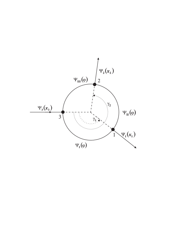
Figure 1: The geometry of the device and the relevant wave functions in the different domains. The parameter $\varphi$ is measured from junction 3 in counterclockwise direction.

where $n=1,2$ label the two outgoing leads.

In order to obtain the transmission matrices, the 12 coefficients $a_{ij}^{\mu}$ have to be determined. This can be done via requiring continuity of the wave functions, and vanishing net spin current densities (Griffith conditions) G53 ; X92 ; MPV04 ; FMBP05 at the three junctions.

According to the detailed calculations presented in the Appendix, the elements of the transmission matrices are:

$$T_{\uparrow\uparrow}^{\left(n\right)} = \frac{8qka}{y}e^{-i\frac{\gamma n}{2}}\left[\cos^{2}\frac{\theta}{2}\left(h_{1}^{\left(n\right)}+h_{2}^{\left(n\right)}\right)+\sin^{2}\frac{\theta}{2}\left(h_{1}^{\left(n\right)}-h_{2}^{\left(n\right)}\right)^{\ast}\right],$$

$$T_{\uparrow\downarrow}^{\left(n\right)} = \frac{8qka}{y}e^{-i\frac{\gamma_{n}}{2}}\sin\frac{\theta}{2}\cos\frac{\theta}{2}\left[\left(h_{1}^{\left(n\right)}+h_{2}^{\left(n\right)}\right)-\left(h_{1}^{\left(n\right)}-h_{2}^{\left(n\right)}\right)^{\ast}\right],$$ (11)

$$T_{\downarrow\uparrow}^{\left(n\right)} = e^{i\gamma_{n}}T_{\uparrow\downarrow}^{\left(n\right)},$$

$$T_{\downarrow\downarrow}^{\left(n\right)} = \frac{8qka}{y}e^{i\frac{\gamma_{n}}{2}}\left[\sin^{2}\frac{\theta}{2}\left(h_{1}^{\left(n\right)}+h_{2}^{\left(n\right)}\right)+\cos^{2}\frac{\theta}{2}\left(h_{1}^{\left(n\right)}-h_{2}^{\left(n\right)}\right)^{\ast}\right],$$

where

$$h_{1}^{\left(1\right)} = -kae^{i\frac{w}{2}\gamma_{1}}\sin\left(q\left(2\pi-\gamma_{2}\right)\right)\sin\left(q\left(\gamma_{2}-\gamma_{1}\right)\right),$$

$$h_{1}^{\left(2\right)} = kae^{i\frac{w}{2}\gamma_{2}}e^{-iw\pi}\sin\left(q\gamma_{1}\right)\sin\left(q\left(\gamma_{2}-\gamma_{1}\right)\right),$$

$$h_{2}^{\left(n\right)} = iqe^{i\frac{w}{2}\gamma_{n}}\left(e^{-iw\pi}\sin\left(q\gamma_{n}\right)-\sin\left(q\left(2\pi-\gamma_{n}\right)\right)\right),$$

and $y$ is given by (Appendix).

The reflection matrix $R$ is found to be diagonal in the $\{\left|\uparrow\right\rangle$, $\left|\downarrow\right\rangle\}$ basis of $S_{z}$:

$$R_{\uparrow\uparrow} = R_{\downarrow\downarrow}=\frac{8ka}{y}\left\{-iq^{2}\sin\left(2q\pi\right)+ik^{2}a^{2}\sin\left(q\left(\gamma_{2}-\gamma_{1}\right)\right)\sin\left(q\left(2\pi-\gamma_{2}\right)\right)\sin\left(q\gamma_{1}\right)\right.$$

$$\left.-qka\left[\sin\left(q\left(2\pi-\gamma_{1}\right)\right)\sin\left(q\gamma_{1}\right)+\sin\left(q\left(2\pi-\gamma_{2}\right)\right)\sin\left(q\gamma_{2}\right)\right]\right\}-1,$$

$$R_{\uparrow\downarrow} = R_{\downarrow\uparrow}=0.$$

This matrix describes the losses in the efficiency of the spin transformation, as the sum of the norms of the outgoing and reflected waves should be equal to the norm of the input.

III Analysis and visualization

When the incoming electron is not perfectly spin-polarized, i.e. its spin state is a mixture, which – instead of a two component spinor – should be described by a $2\times 2$ density matrix $\varrho_{in}$, then we can readily generalize equation (10) to obtain

$$\varrho^{\left(n\right)}=T^{\left(n\right)}\varrho_{in}\left(T^{\left(n\right)}\right)^{\dagger},$$

where $\varrho^{\left(1\right)}$ and $\varrho^{\left(2\right)}$ are the output density matrices in the respective leads.

Considering a completely unpolarized input, i.e. $\varrho_{in}$ being proportional to the $2\times 2$ identity matrix, in order to get polarized outputs, the relevant output density operators should be projectors (apart from the possible reflective losses):

$$\frac{1}{2}T^{\left(n\right)}\left(T^{\left(n\right)}\right)^{\dagger}=\eta_{n}\left|\phi^{n}\right\rangle\left\langle\phi^{n}\right|.$$ (12)

The non-negative numbers $\eta_{1}$ and $\eta_{2}$ measure the efficiency of the polarizing device, i.e. $\eta_{1}+\eta_{2}=1$ means a reflectionless process. Equation (12) is equivalent to require that the determinants of $T^{\left(n\right)}\left(T^{\left(n\right)}\right)^{\dagger}$ vanish. According to equations (11) there are two different conditions for each transmission matrix to satisfy this requirement:

$$h_{1}^{\left(n\right)}\pm h_{2}^{\left(n\right)}=0,$$ (13)

where $n=1,2$ indicates the two output juctions. It can be shown that only the following two cases lead to nonzero transmission at both outputs:

$$h_{1}^{\left(1\right)}+h_{2}^{\left(1\right)} = 0,$$

$$h_{1}^{\left(2\right)}-h_{2}^{\left(2\right)} = 0,$$ (14a)

or

$$h_{1}^{\left(1\right)}-h_{2}^{\left(1\right)} = 0,$$

$$h_{1}^{\left(2\right)}+h_{2}^{\left(2\right)} = 0.$$ (14b)

After substitution we obtain two equations for $$\cos\left(w\pi\right) \sin\left(w\pi\right)$$ and in both cases:

$$\cos\left(w\pi\right)\! = \!\frac{\sin\left(q\left(2\pi-\gamma_{1}\right)\right)}{\sin\left(q\gamma_{1}\right)}\!=\!\frac{\sin\left(q\gamma_{2}\right)}{\sin\left(q\left(2\pi-\gamma_{2}\right)\right)},$$ (15a)

$$\sin\left(w\pi\right)\! = \!\pm\frac{ka}{q}\frac{\sin\left(q\left(2\pi-\gamma_{2}\right)\right)\sin\left(q\left(\gamma_{2}-\gamma_{1}\right)\right)}{\sin\left(q\gamma_{1}\right)}\!=\!\pm\frac{ka}{q}\frac{\sin\left(q\gamma_{1}\right)\sin\left(q\left(\gamma_{2}-\gamma_{1}\right)\right)}{\sin\left(q\left(2\pi-\gamma_{2}\right)\right)},$$ (15b)

or with the Aharonov-Casher phase

$$\cos\Phi^{\left(\mu\right)}\! = \!-\!\frac{\sin\left(q\left(2\pi-\gamma_{1}\right)\right)}{\sin\left(q\gamma_{1}\right)}\!=\!-\!\frac{\sin\left(q\gamma_{2}\right)}{\sin\left(q\left(2\pi-\gamma_{2}\right)\right)},$$ (16a)

$$\sin\Phi^{\left(\mu\right)}\! = \!\pm\left(-1\right)^{\mu}\frac{ka}{q}\frac{\sin\left(q\left(2\pi-\gamma_{2}\right)\right)\sin\left(q\left(\gamma_{2}-\gamma_{1}\right)\right)}{\sin\left(q\gamma_{1}\right)}\!$$ (16b)

$$= \!\pm\left(-1\right)^{\mu}\frac{ka}{q}\frac{\sin\left(q\gamma_{1}\right)\sin\left(q\left(\gamma_{2}-\gamma_{1}\right)\right)}{\sin\left(q\left(2\pi-\gamma_{2}\right)\right)},$$

where the plus sign in (15b) corresponds to equation (14a), while the minus sign is for the case given by equation (14b). From (15a) and (15b) for both signs we find

$$\sin\left(q\gamma_{1}\right) = \pm\sin\left(q\left(2\pi-\gamma_{2}\right)\right),$$

$$\sin\left(q\gamma_{2}\right) = \pm\sin\left(q\left(2\pi-\gamma_{1}\right)\right).$$

The solutions of these equations for a fixed $\gamma_{2}$ are

$$\gamma_{1}=2\pi-\gamma_{2}\pm m\pi/q,$$ (17)

or for a fixed $\gamma_{1}$ are

$$\gamma_{2}=2\pi-\gamma_{1}\pm l\pi/q,$$ (18)

where $m,l$ are nonnegative integers which ensure $0\!\leq\!\gamma_{1,}\gamma_{2}\!\leq\!2\pi$ and $\gamma_{2}\!\geq\!\gamma_{1}$. The $m,l=0$ cases correspond to a ring the outgoing leads of which are symmetric with respect to the incoming lead. It was demonstrated that for such a ring one can find lines in the $\{\gamma_{2},\omega/\Omega,ka\}$ space along which the conditions (15a) and (15b) can be satisfied FKBP06 , i.e. the ring polarizes a completely unpolarized input. Polarization occurs with equal $\eta_{1}=\eta_{2}\equiv\eta/2$ transmission in both outputs. Parameter combinations, for which the transmission probability $\eta$ is unity can also be found.

From equations (17) and (18) we see that we can extend the polarizing property to asymmetric geometries. The asymmetric positions of the two output leads for which the condition for complete spin polarization is satisfied are $\pm l\pi/q$ and $\pm m\pi/q$ angles away from the symmetric ones. For proper combinations of the $\omega/\Omega$ and $ka$ parameters the asymmetric ring also produces polarized outputs with equal transmission probabilities $\eta_{1}=\eta_{2}=128q^{2}k^{2}a^{2}\left|h_{1}^{\left(1\right)}\right|^{2}/\left|y\right|^{2}$. We note that this is an important generalization of the results of Ref. FKBP06 . There are several appropriate positions for the output leads, the symmetric case is just one of them.

The output spinors are the eigenstates $\left|\phi^{n}\right\rangle$ of the transmitted density matrices $\frac{1}{2}T^{\left(n\right)}\left(T^{\left(n\right)}\right)^{\dagger}$, which correspond to the nonzero eigenvalues given by $\eta_{n}$. Focusing on the case of equations (14a), these eigenstates read

$$\left|\phi_{a}^{1}\right\rangle=\begin{pmatrix}e^{-i\frac{\gamma_{1}}{2}}\sin\frac{\theta}{2}\\ -e^{i\frac{\gamma_{1}}{2}}\cos\frac{\theta}{2}\end{pmatrix},\quad\left|\phi_{a}^{2}\right\rangle=\begin{pmatrix}e^{-i\frac{\gamma_{2}}{2}}\cos\frac{\theta}{2}\\ e^{i\frac{\gamma_{2}}{2}}\sin\frac{\theta}{2}\end{pmatrix}.$$ (19)

These results describe the connection between the strength of the spin-orbit coupling (encoded in $\theta$), the geometry of the device and its polarizing directions. Note that these spinors are in general non-orthogonal, their overlap is given by $\left\langle\phi^{2}\right|\left.\phi^{1}\right\rangle=i\sin\theta\sin{(\gamma_{2}-\gamma_{1})/2}$. For the other case given by equations (14b) we have:

$$\left|\phi_{b}^{1}\right\rangle=\begin{pmatrix}e^{-i\frac{\gamma_{1}}{2}}\cos\frac{\theta}{2}\\ e^{i\frac{\gamma_{1}}{2}}\sin\frac{\theta}{2}\end{pmatrix},\quad\left|\phi_{b}^{2}\right\rangle=\begin{pmatrix}e^{-i\frac{\gamma_{2}}{2}}\sin\frac{\theta}{2}\\ -e^{i\frac{\gamma_{2}}{2}}\cos\frac{\theta}{2}\end{pmatrix}.$$ (20)

We can see from (19) and (20) that the output spin states in both cases are the two eigenspinors of the Hamiltonian at the positions of the output junctions. For a given output lead, the two eigenspinors are interchanged in the two cases.

Figure 2: Transmission probability $\eta=2\eta_{1}=2\eta_{2}$ at the two outputs of an asymmetric ring as a function of $ka$ for $\omega/\Omega=2.27$. This figure corresponds to $\gamma_{2}=4\pi/3$ and $\gamma_{1}=2\pi-\gamma_{2}-6\pi/q$. The dots mark the points where perfect polarization occurs.

Figure 2 shows this transmission probability as a function of $ka$ for $\omega/\Omega=2.27$. The dots on the curve mark the points where perfect polarization occurs. Since the angle $\gamma_{1}$ is a function of $ka$, the dots correspond to different asymmetric configurations. It can be seen that even for an asymmetric ring, with appropriate parameter values, complete output spin polarization can be achieved with practically zero reflective loss.

Now we investigate the physical origin of this polarizing effect. To this end we consider a completely unpolarized input taken as the following equal weight sum of pure state projectors

$$\varrho_{in}=\frac{1}{2}\left(\left|\psi_{in}^{1}\right\rangle\left\langle\psi_{in}^{1}\right|+\left|\psi_{in}^{2}\right\rangle\left\langle\psi_{in}^{2}\right|\right).$$

Here $\psi_{in}^{\mu}=\psi_{1}^{\mu}(0)=\psi_{2}^{\mu}(0)$ ($\mu=1,2$), given by equations (7) and (8), are the eigenspinors of the Hamiltonian at the position of the incoming lead (3). The density operator in the different sections of the ring is then

$$\varrho_{i}\left(\varphi\right)=\frac{1}{2}\left(\left|\Psi_{i}^{1}\left(\varphi\right)\right\rangle\left\langle\Psi_{i}^{1}\left(\varphi\right)\right|+\left|\Psi_{i}^{2}\left(\varphi\right)\right\rangle\left\langle\Psi_{i}^{2}\left(\varphi\right)\right|\right)\qquad i=I,I\!I,I\!I\!I,$$ (21)

where

$$\Psi_{i}^{1}\left(\varphi\right) = \sum_{j=1,2}\Psi_{ij}^{1}\left(\varphi\right)=N_{i}^{1}\left(\varphi\right)\begin{pmatrix}e^{-i\frac{\varphi}{2}}\cos\frac{\theta}{2}\\ e^{i\frac{\varphi}{2}}\sin\frac{\theta}{2}\end{pmatrix},$$

$$\Psi_{i}^{2}\left(\varphi\right) = \sum_{j=1,2}\Psi_{ij}^{2}\left(\varphi\right)=N_{i}^{2}\left(\varphi\right)\begin{pmatrix}e^{-i\frac{\varphi}{2}}\sin\frac{\theta}{2}\\ -e^{i\frac{\varphi}{2}}\cos\frac{\theta}{2}\end{pmatrix},$$ (22)

are the spinor valued wave functions of the electron in the different domains of the ring for the pure inputs $\psi_{in}^{1}$ and $\psi_{in}^{2}$ respectively, with

$$N_{i}^{\mu}\left(\varphi\right)=\sum\limits_{j=1,2}a_{ij}^{\mu}e^{i\kappa_{j}^{\mu}\varphi},\qquad\mu=1,2.$$

We can see that for these inputs the wave functions in the ring contain only two of the four eigenstates of the Hamiltonian, those which have the same spinor part.

By calculating the spin current densities corresponding to the $\Psi_{ij}^{\mu}\left(\varphi\right)$ states appearing in (22) we obtain

$$J_{ij}^{\mu}=\left|a_{ij}^{\mu}\right|^{2}\left[2\kappa_{j}^{\mu}+\left(-1\right)^{\mu}\left(\cos\theta-\frac{\omega}{\Omega}\sin\theta\right)\right]=\left(-1\right)^{\mu+j+1}2q\left|a_{ij}^{\mu}\right|^{2}.$$ (23)

By examining (23) we find that $\Psi_{i1}^{\mu}\left(\varphi\right)$ and $\Psi_{i2}^{\mu}\left(\varphi\right)$ represent oppositely directed (clockwise and anticlockwise) spin currents in each section (identified by the index $i$) of the ring, since $J_{i1}^{\mu}$ and $J_{i2}^{\mu}$ have opposite signs. The overall spin current densities – containing both clockwise and anticlockwise directed currents – which correspond to the input $\psi_{in}^{\mu}$ are

$$J_{i}^{\mu}\! = \!2q\!\left(-1\right)^{\mu}\!\left(\!\left|a_{i1}^{\mu}\right|^{2}\!-\!\left|a_{i2}^{\mu}\right|^{2}\!\right)\!+\!2\mathrm{Re}\!\left(\!a_{i1}^{\mu}\left(a_{i2}^{\mu}\right)^{\ast}e^{i\left(\kappa_{1}^{\mu}-\kappa_{2}^{\mu}\right)\varphi}\!\right)\left[\!\kappa_{1}^{\mu}\!+\!\kappa_{2}^{\mu}\!+\!\left(-1\right)^{\mu}\!\left(\!\cos\theta\!-\!\frac{\omega}{\Omega}\sin\theta\!\right)\!\right]$$ (24)

$$= \!2q\left(-1\right)^{\mu}\!\left(\!\left|a_{i1}^{\mu}\right|^{2}\!-\!\left|a_{i2}^{\mu}\right|^{2}\!\right)=J_{i1}^{\mu}-J_{i2}^{\mu}.$$

We note that the disappearance of the cross terms in (24) is due to the fact that $\tan\theta=-\omega/\Omega$.

The output spinors given by (19) and (20) suggest, that in order to obtain a polarized (pure) state at a given output, we need one of the one-dimensional projectors of (21) to vanish, and the other one to remain nonzero at that point of the ring. In order to have different polarized spin states in both outputs, the two projectors need to vanish at the different output junctions. One of the possible ways to achieve this is to have $\Psi_{I}^{1}\left(\gamma_{1}\right)$ and $\Psi_{II}^{1}\left(\gamma_{2}\right)$ being zero, which happens if the spatial parts of these wave functions are zero (see equations (22)):

$$N_{I}^{1}\left(\gamma_{1}\right)=0,\qquad N_{II}^{2}\left(\gamma_{2}\right)=0,$$ (25)

indicating destructive interference at the given output. By exchanging $\mu\!=\!1$ and $\mu\!=\!2$, we can describe the other case of polarization. Condition (25) can be satisfied if

$$\left|a_{I,1}^{1}\right|=\left|a_{I,2}^{1}\right|,\qquad\left|a_{I\!I,1}^{2}\right|=\left|a_{I\!I,2}^{2}\right|,$$ (26)

which, by using equation (52), can be shown to be equivalent to equations (14a). (Exchanging $\mu\!=\!1$ and $\mu\!=\!2$ in (25) leads to (14b)). Equation (26) implies that the spin currents $J_{I}^{1}$ and $J_{I\!I}^{2}$ given by (24) vanish as a consequence of the interference of oppositely directed currents corresponding to states of the same spinor parts. We can see that the requirement for spin-polarization given by (12), has a very clear physical interpretation in terms of destructive interference and vanishing spin currents.

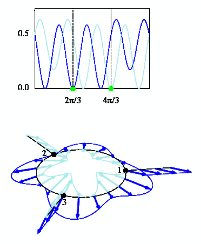
Figure 3: The stationary spin directions of the electron along the (symmetric) ring for a completely unpolarized input given by $\varrho_{in}=\frac{1}{2}\left(\left|\psi_{in}^{1}\right\rangle\left\langle\psi_{in}^{1}\right|+\left|\psi_{in}^{2}\right\rangle\left\langle\psi_{in}^{2}\right|\right)$  with $\gamma_{2}=4\pi/3$, $\omega/\Omega=3.05$, $ka=1.38$ note2 , which ensure perfect polarization in the case given by equation (14a). Light and dark (blue online) arrows correspond to $\psi_{in}^{1}$ and $\psi_{in}^{2}$ respectively. The length of the arrows as well as the curves with the corresponding colour on the upper graph show the probabilities of finding the electron at the given point on the ring. The dashed lines in the upper graph mark the outgoing leads, where one of the two probabilities becomes zero, resulting in the output of the other spinor as a pure state. The two outputs in this case are given by equations (19).

Figure 3 and the corresponding animation show the stationary spin directions of the electron along the ring for a completely unpolarized input, for parameter values which ensure perfect polarization at the outputs (in the case given by (14a) for a symmetric ring). Light and dark (blue online) arrows correspond to $\psi_{in}^{1}$ and $\psi_{in}^{2}$, respectively. The length of the arrows as well as the curves with the corresponding colour on the upper graph show the probabilities of finding the electron at the given point on the ring. The dashed lines in the upper graph mark the outgoing leads, where one of the two probabilities becomes zero, leading to the output of the other spinor, given by equation (19). We note that spin transformation in this case is a rotation around the z-axis by an angle pertaining to the given point on the ring.

It is also interesting to see how polarization is produced if we decompose the incoming perfect mixture as an equal weight sum of the eigenstates of $S_{z}$

$$\varrho_{in}=\frac{1}{2}\left(\left|\uparrow\right\rangle\left\langle\uparrow\right|+\left|\downarrow\right\rangle\left\langle\downarrow\right|\right).$$

Figure 4 and the corresponding animation show the stationary spin directions along the ring for such an input and for the same parameter values as in figure 3. Light and dark (blue online) arrows correspond to inputs $\left|\uparrow\right\rangle$ and $\left|\downarrow\right\rangle$, respectively. The outgoing arrows (green online) represent the output spinors given by equations (19). The spin direction of the electron in the two branches of the ring is illustrated on the two Bloch spheres NC00 above the ring, where the length of the black arrow represents the purity of the given state. When the arrow reaches the surface, the spin state is pure, otherwise it is mixed, zero length meaning a perfect mixture. The dots on the Bloch spheres (green online) indicate that at the positions of the output junctions the states are pure. The animation shows that the $\left|\uparrow\right\rangle$ and $\left|\downarrow\right\rangle$ inputs are rotated into the same direction at the outputs of the ring, resulting in the same pure states as those seen in figure 3.

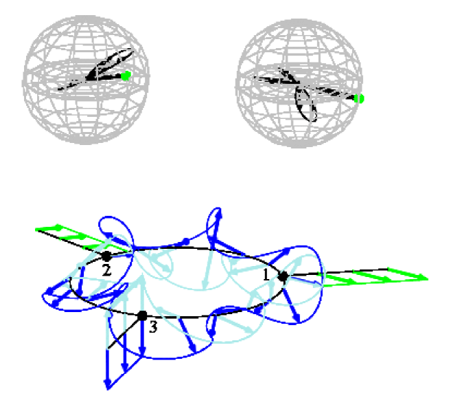
Figure 4: The stationary spin directions along the ring for a completely unpolarized input given by $\varrho_{in}=\frac{1}{2}\left(\left|\uparrow\right\rangle\left\langle\uparrow\right|+\left|\downarrow\right\rangle\left\langle\downarrow\right|\right)$, for the same parameter values as for figure 3. Light and dark (blue online) arrows correspond to inputs $\left|\uparrow\right\rangle$ and $\left|\downarrow\right\rangle$  respectively. The outgoing arrows (green online) represent the output spinors given by equations (19). The spin state of the electron in left (right) branch of the ring is illustrated on the Bloch spheres NC00 above the respective part of the ring. At the positions of the output junctions the black arrows reach the surface of the spheres – denoted by the dots (green online) – indicating that the state at those points is pure. The animation shows that the $\left|\uparrow\right\rangle$ and $\left|\downarrow\right\rangle$ inputs are rotated into the same direction at the outputs of the ring.

The role of spin-orbit interaction in the polarizing process can also be seen in figures 3 and 4. The spin-sensitivity of the problem leads to a symmetry Y06 of the stationary solution that is more complex than the pure geometrical mirror transformation. Note that without spin-orbit interaction destructive interference for a given spin direction would imply that the orthogonal spin component of the wave function is also zero at that point. Consequently placing the output junctions in such positions would mean zero transmission probability. This can also be seen by considering that the rotation of the $\left|\uparrow\right\rangle$ and $\left|\downarrow\right\rangle$ spinors shown in figure 4 is due to spin-orbit interaction, for $\omega=0$ (or $\Phi=0$) their direction in the ring would not change, i.e., they could never precess into the same direction.

Figure 3 and 4 show that besides the actual output junctions, which are situated symmetric with respect to the incoming lead, there are additional points on both branches of the ring where the state of the electron is pure. These points are situated asymmetric with respect to the incoming lead, and can be determined from equations (17) and (18). If the output leads are put into those positions, the outcoming spins states are the ones given by (19).

IV Conclusions

We considered a three-terminal quantum ring with one input and two output leads, which for appropriate parameter values acts as a spin polarizer, similarly to the Stern-Gerlach apparatus. We presented a detailed analytic solution of the spin-dependent transport problem and provided the physical interpretation of the process: For both symmetric and non-symmetric geometries, polarization is due to spatial interference. At a given junction this interference is destructive for a certain spin direction, while constructive for its orthogonal counterpart, which, consequently is transmitted into the output lead.

Appendix

Considering the input junction, the continuity and Griffith conditions read:

$$\Psi_{3}\left(0\right)=\Psi_{I}\left(0\right)=\Psi_{I\!I\!I}\left(2\pi\right),$$ (27)

$$J_{3}\left(0\right)-J_{I}\left(0\right)+J_{I\!I\!I}\left(2\pi\right)=0,$$ (28)

respectively. Analogous equations can be written for the other two junctions. The appropriately normalized spin current densities in the leads are given by

$$J_{l}\left(x_{l}\right)=2a\mathrm{Re}\left(\Psi_{l}^{\dagger}\left(x_{l}\right)\left(-i\frac{\partial}{\partial x_{l}}\right)\Psi_{l}\left(x_{l}\right)\right),$$ (29)

and in the ring by MPV04

$$J_{i}\left(\varphi\right)=2\mathrm{Re}\left[\Psi_{i}^{\dagger}\left(\varphi\right)\left(\frac{\omega}{2\Omega}\sigma_{r}\left(\varphi\right)-i\frac{\partial}{\partial\varphi}\right)\Psi_{i}\left(\varphi\right)\right],$$ (30)

where $\sigma_{r}\left(\varphi\right)=\cos\varphi\sigma_{x}+\sin\varphi\sigma_{y}$, $i=I,I\!I,I\!I\!I$ and $l=1,2,3$. For the sake of definiteness, we present the details for the incoming junction (3). The results for the other junctions can be obtained in a similar manner.

First, we simplify equation (28) by using (29) and (30)

$$a\left.\frac{\partial\Psi_{3}}{\partial x_{3}}\right|_{x_{3}=0}-\left.\frac{\partial\Psi_{I}}{\partial\varphi}\right|_{\varphi=0}+\left.\frac{\partial\Psi_{I\!I\!I}}{\partial\varphi}\right|_{\varphi=2\pi}=0.$$ (31)

Substituting the wave functions (5) and (9) into (27) we get

$$f_{\uparrow}+r_{\uparrow} = \sum\limits_{\mu,j}a_{I,j}^{\mu}u_{j}^{\mu}=-\sum\limits_{\mu,j}a_{I\!I\!I,j}^{\mu}e^{i\kappa_{j}^{\mu}2\pi}u_{j}^{\mu},$$ (32)

$$f_{\downarrow}+r_{\downarrow} = \sum\limits_{\mu,j}a_{I,j}^{\mu}v_{j}^{\mu}=-\sum\limits_{\mu,j}a_{I\!I\!I,j}^{\mu}e^{i\kappa_{j}^{\mu}2\pi}v_{j}^{\mu}.$$ (33)

The same substitution in (31) yields

$$f_{\uparrow}-r_{\uparrow} = \sum\limits_{\mu,j}\beta_{j}^{\mu}\left(a_{I,j}^{\mu}+a_{I\!I\!I,j}^{\mu}e^{i\kappa_{j}^{\mu}2\pi}\right)u_{j}^{\mu},$$ (34)

$$f_{\downarrow}-r_{\downarrow} = \sum\limits_{\mu,j}\gamma_{j}^{\mu}\left(a_{I,j}^{\mu}+a_{I\!I\!I,j}^{\mu}e^{i\kappa_{j}^{\mu}2\pi}\right)v_{j}^{\mu},$$ (35)

where $\beta_{j}^{\mu}=\left(\kappa_{j}^{\mu}-\frac{1}{2}\right)/ka$ and $\gamma_{j}^{\mu}=\left(\kappa_{j}^{\mu}+\frac{1}{2}\right)/ka$. Since our aim is to determine the $a_{ij}^{\mu}$ coefficients, we eliminate $r_{\uparrow}$ and $r_{\downarrow}$

$$\sum\limits_{\mu,j}\left(a_{I,j}^{\mu}+a_{I\!I\!I,j}^{\mu}e^{i\kappa_{j}^{\mu}2\pi}\right)u_{j}^{\mu} = 0,$$ (36)

$$\sum\limits_{\mu,j}\left(a_{I,j}^{\mu}+a_{I\!I\!I,j}^{\mu}e^{i\kappa_{j}^{\mu}2\pi}\right)v_{j}^{\mu} = 0,$$ (37)

$$\sum\limits_{\mu,j}\left[\beta_{j}^{\mu}\left(a_{I,j}^{\mu}+a_{I\!I\!I,j}^{\mu}e^{i\kappa_{j}^{\mu}2\pi}\right)+a_{I,j}^{\mu}\right]u_{j}^{\mu} = 2f_{\uparrow},$$ (38)

$$\sum\limits_{\mu,j}\left[\gamma_{j}^{\mu}\left(a_{I,j}^{\mu}+a_{I\!I\!I,j}^{\mu}e^{i\kappa_{j}^{\mu}2\pi}\right)+a_{I,j}^{\mu}\right]v_{j}^{\mu} = 2f_{\downarrow}.$$ (39)

After substituting the $u_{j}^{\mu}$ and $v_{j}^{\mu}$ spinor components given by (7) and (8) into (36)-(39) we find

$$\sum\limits_{j}\left[\left(a_{I,j}^{1}+a_{I\!I\!I,j}^{1}e^{i\kappa_{j}^{1}2\pi}\right)\cos\frac{\theta}{2}+\left(a_{I,j}^{2}+a_{I\!I\!I,j}^{2}e^{i\kappa_{j}^{2}2\pi}\right)\sin\frac{\theta}{2}\right] = 0,$$ (40)

$$\sum\limits_{j}\left[\left(a_{I,j}^{1}+a_{I\!I\!I,j}^{1}e^{i\kappa_{j}^{1}2\pi}\right)\sin\frac{\theta}{2}-\left(a_{I,j}^{2}+a_{I\!I\!I,j}^{2}e^{i\kappa_{j}^{2}2\pi}\right)\cos\frac{\theta}{2}\right] = 0,$$ (41)

$$\sum\limits_{j}\left\{\left[\beta_{j}^{1}\!\left(a_{I,j}^{1}\!+\!a_{I\!I\!I,j}^{1}e^{i\kappa_{j}^{1}2\pi}\right)\!+\!a_{I,j}^{1}\right]\cos\frac{\theta}{2}\!+\!\left[\beta_{j}^{2}\!\left(a_{I,j}^{2}\!+\!a_{I\!I\!I,j}^{2}e^{i\kappa_{j}^{2}2\pi}\right)\!+\!a_{I,j}^{2}\right]\sin\frac{\theta}{2}\right\}\! = \!2f_{\uparrow},$$ (42)

$$\sum\limits_{j}\left\{\left[\gamma_{j}^{1}\!\left(a_{I,j}^{1}\!+\!a_{I\!I\!I,j}^{1}e^{i\kappa_{j}^{1}2\pi}\right)\!+\!a_{I,j}^{1}\right]\sin\frac{\theta}{2}\!-\!\left[\gamma_{j}^{2}\!\left(a_{I,j}^{2}\!+\!a_{I\!I\!I,j}^{2}e^{i\kappa_{j}^{2}2\pi}\right)\!+\!a_{I,j}^{2}\right]\cos\frac{\theta}{2}\right\}\! = \!2f_{\downarrow}.$$ (43)

Notice that certain terms can be cancelled out by using simple trigonometric identities, giving:

$$\sum\limits_{j}\left(a_{I,j}^{1}+a_{I\!I\!I,j}^{1}e^{i\kappa_{j}^{1}2\pi}\right) = 0,$$ (44)

$$\sum\limits_{j}\left(a_{I,j}^{2}+a_{I\!I\!I,j}^{2}e^{i\kappa_{j}^{2}2\pi}\right) = 0,$$ (45)

$$\sum\limits_{j}\left[\left(2\kappa_{j}^{1}-\cos\theta\right)\left(a_{I,j}^{1}+a_{I\!I\!I,j}^{1}e^{i\kappa_{j}^{1}2\pi}\right)+2kaa_{I,j}^{1}-\sin\theta\left(a_{I,j}^{2}+a_{I\!I\!I,j}^{2}e^{i\kappa_{j}^{2}2\pi}\right)\right] = 2d^{1},$$ (46)

$$\sum\limits_{j}\left[\left(2\kappa_{j}^{2}+\cos\theta\right)\left(a_{I,j}^{2}+a_{I\!I\!I,j}^{2}e^{i\kappa_{j}^{2}2\pi}\right)+2kaa_{I,j}^{2}-\sin\theta\left(a_{I,j}^{1}+a_{I\!I\!I,j}^{1}e^{i\kappa_{j}^{1}2\pi}\right)\right] = 2d^{2},$$ (47)

where

$$d^{1} = 2ka\left(\cos\frac{\theta}{2}f_{\uparrow}+\sin\frac{\theta}{2}f_{\downarrow}\right),$$ (48)

$$d^{2} = 2ka\left(\sin\frac{\theta}{2}f_{\uparrow}-\cos\frac{\theta}{2}f_{\downarrow}\right).$$ (49)

The sums in equations (46) and (47) can be simplified using (44) and (45):

$$\sum\limits_{j}\left[\left(2\kappa_{j}^{1}+2ka\right)a_{I,j}^{1}+2\kappa_{j}^{1}a_{I\!I\!I,j}^{1}e^{i\kappa_{j}^{1}2\pi}\right] = 2d^{1},$$ (50)

$$\sum\limits_{j}\left[\left(2\kappa_{j}^{2}+2ka\right)a_{I,j}^{2}+2\kappa_{j}^{2}a_{I\!I\!I,j}^{2}e^{i\kappa_{j}^{2}2\pi}\right] = 2d^{2}.$$ (51)

Thus, the equations originating from the continuity requirements at the incoming junction (3) (see figure 1) split into two separate systems for $\mu=1,2$.

The other two junctions lead to four additional equations and consequently we have to solve six equations for six unknowns for each $\mu$. We can start by expressing $a_{I\!I\!I,j}^{1}$ by $a_{I,j}^{1}$ from equations (44) and (46), and also by $a_{I\!I,j}^{1}$ from the equations for junction 2. Using these two expressions for $a_{I\!I\!I,j}^{1}$ we obtain a relation between $a_{I\!I,j}^{1}$ and $a_{I,j}^{1}$. From the equations of the first outgoing junction we can also express $a_{I\!I,j}^{1}$ in terms of $a_{I,j}^{1}$. Finally, we can use the two different expressions for $a_{I\!I,j}^{1}$ to calculate $a_{I,j}^{1}$. This automatically determines all the other coefficients (since we have these expressed by $a_{I,j}^{1}$). The $\mu=2$ case can be solved analogously. The twelve $a_{ij}^{\mu}$ coefficients read

$$a_{I,j}^{\mu} = \frac{2d^{\mu}}{y}\left(-1\right)^{\mu+j}\left\{k^{2}a^{2}e^{i\left(-1\right)^{\mu+j}q\gamma_{1}}\sin\left(q\left(\gamma_{2}-\gamma_{1}\right)\right)\sin\left(q\left(2\pi-\gamma_{2}\right)\right)\right.$$

$$\left.+iqka\left[e^{i\left(-1\right)^{\mu+j}q\gamma_{1}}\sin\left(q\left(2\pi-\gamma_{1}\right)\right)+e^{i\left(-1\right)^{\mu+j}q\gamma_{2}}\sin\left(q\left(2\pi-\gamma_{2}\right)\right)\right]\right.$$

$$\left.-q^{2}\left(e^{i\left(-1\right)^{\mu}w\pi}+e^{i\left(-1\right)^{\mu+j}q2\pi}\right)\right\},$$

$$a_{I\!I,j}^{\mu} = \frac{2qd^{\mu}}{y}\left(-1\right)^{\mu+j}\left\{-q\left(e^{i\left(-1\right)^{\mu}w\pi}+e^{i\left(-1\right)^{\mu+j}q2\pi}\right)\right.$$

$$\left.+ika\left[e^{i\left(-1\right)^{\mu+j}q\gamma_{1}}e^{i\left(-1\right)^{\mu}w\pi}\sin\left(q\gamma_{1}\right)+e^{i\left(-1\right)^{\mu+j}q\gamma_{2}}\sin\left(q\left(2\pi-\gamma_{2}\right)\right)\right]\right\},$$

$$a_{I\!I\!I,j}^{\mu} = \frac{1}{2q}\left[\left(2q+\left(-1\right)^{\mu+j}ka\right)a_{I\!I,j}^{\mu}+\left(-1\right)^{\mu+j}kae^{2i\left(-1\right)^{\mu+j}q\gamma_{2}}a_{I\!I,j+\left(-1\right)^{j+1}}^{\mu}\right],$$ (52)

where

$$y = ik^{3}a^{3}\left[\sin\left(2q\left(\pi-\gamma_{2}+\gamma_{1}\right)\right)+\sin\left(2q\left(\pi-\gamma_{1}\right)\right)-\sin\left(2q\left(\pi-\gamma_{2}\right)\right)-\sin\left(2q\pi\right)\right]$$

$$-2qk^{2}a^{2}\left[\cos\left(2q\left(\pi-\gamma_{2}+\gamma_{1}\right)\right)+\cos\left(2q\left(\pi-\gamma_{1}\right)\right)+\cos\left(2q\left(\pi-\gamma_{2}\right)\right)-\cos\left(2q\pi\right)\right]$$

$$+4qk^{2}a^{2}\cos\left(2q\pi\right)-12iq^{2}ka\sin\left(2q\pi\right)+8q^{3}\left[\cos\left(w\pi\right)+\cos\left(2q\pi\right)\right].$$

The elements of the transmission matrices can be determined from the continuity equations $t_{1}^{\left(n\right)}=\sum\limits_{\mu,j}a_{I\!I,j}^{\mu}e^{i\left(\kappa_{j}^{\mu}-\frac{1}{2}\right)\gamma_{n}}u_{j}^{\mu}$ and $t_{2}^{\left(n\right)}=\sum\limits_{\mu,j}a_{I\!I,j}^{\mu}e^{i\left(\kappa_{j}^{\mu}+\frac{1}{2}\right)\gamma_{n}}v_{j}^{\mu}$ at the outgoing junctions (1 and 2) yielding (11).

References

• (1) Žutić I, Fabian J and Sarma S D 2004 Rev. Mod. Phys. 76 323
• (2) Rashba E I 1960 Sov. Phys. Solid State 2 1109
• (3) Nitta J, Akazaki T, Takayanagi H and Enoki T 1997 Phys. Rev. Lett.  78 1335
• (4) Földi P, Molnár B, Benedict M G and Peeters F M 2005 Phys. Rev. B 71 033309
• (5) Aronov A G and Lyanda-Geller Y B 1993 Phys. Rev. Lett. 70 343
• (6) Nitta J, Meijer F E and Takayanagi H 1999 Appl. Phys. Lett. 75 695
• (7) Büttiker M, Imry Y and Azbel M Ya 1984 Phys. Rev. A 30 1982
• (8) Vasilopoulos P, Kálmán O, Benedict M G and Peeters F M 2006 to appear in Phys. Rev. B
• (9) Koga T, Nitta J and van Veenhuizen M 2004 Phys. Rev. B 70 161302(R)
• (10) Sato Y, Kita S G T and Yamada S 2001 J. Appl. Phys. 89 8017
• (11) Molnár B, Peeters F M and Vasilopoulos P 2004 Phys. Rev. B 69 155335
• (12) Frustaglia D and Richter K 2004 Phys. Rev. B 69 235310
• (13) Zhai F and Xu H Q 2005 Phys. Rev. Lett. 94 246601
• (14) Ionicioiu R and D’Amico I 2003 Phys. Rev. B 67 041307 (R)
• (15) Governale M, Boese D, Zülicke U and Schroll C 2002 Phys. Rev. B 65 140403 (R)
• (16) König M, Tschetschetkin A, Hankiewicz E M, Sinova J, Hock V, Daumer V, Schäfer M, Becker C R, Buhmann H and Molenkamp L W 2006 Phys. Rev. Lett. 96 076804
• (17) Souma S and Nikolić B 2005 Phys. Rev. Lett. 94 106602
• (18) Kato Y K, Myers R C, Gossard A C and Awschalom D D 2005 Appl. Phys. Lett. 86 162107
• (19) Cserti J, Csordás A and Zülicke U 2004 Phys. Rev. B 70 233307
• (20) Pályi A, Péterfalvi C and Cserti J 2006 Phys. Rev. B 74 073305
• (21) Euges J C, Burkard G and Loss D 2003 Appl. Phys. Lett. 82 2658
• (22) Stepanenko D, Bonesteel N E, DiVincenzo D P, Burkard G and Loss D 2003  Appl. Phys. Lett. 68 115306
• (23) Yau J B, DePoortere E P and Shayegan M 2003 Phys. Rev. Lett. 88 146801
• (24) Frustaglia D, Hentschel M and Richter K 2001 Phys. Rev. Lett. 87 256602
• (25) Földi P, Kálmán O, Benedict M G and Peeters F M 2006 Phys. Rev. B 73 155325
• (26) Mott N F and Massey H S W 1949 The theory of atomic collissions 2nd ed (Oxford: Clarendon Press)
• (27) Pareek T P 2004 Phys. Rev. Lett. 92 076601
• (28) Note that entanglement—in the strict sense—is a strong quantum mechanical correlation of two or more different particles. The effect, when the different degrees of freedom of a single particle become entangled (see e.g.: Y. Hasegawa and R. Loidl and G. Badurek and M. Baron and H. Rauch, Nature (London) 425 45 (2003)), can be called intertwining.
• (29) Kálmán O, Földi P and Benedict M G 2006 Open Sys. & Inf. Dyn. 13 455
• (30) Aharonov Y and Casher A 1984 Phys. Rev. Lett. 53 319
• (31) Meijer F E, Morpugo A F and Klapwijk T M 2002 Phys. Rev. B 66 033107
• (32) Griffith S 1953 Trans. Faraday Soc. 49 345
• (33) Xia J B 1992 Phys. Rev. B 45 3593
• (34) We note that in semiconductor rings, the actual value of $ka$ is usually an order of magnitude larger, e.g. in a ring of radius $0.25\mu$m made of InGaAs, where the Fermi energy is $11.13$ meV, one has $k_{F}a\approx 20.4$. The experimentally feasible value of $\omega/\Omega$ is around $1$. The values used here are to provide a better visualization of the phenomenon.
• (35) Nielsen M A and Chuang I L 2000 Quantum computation and quantum information (Cambridge: Cambridge Univ. Press)
• (36) Yang S R E 2006 Phys. Rev. B 74 075315