Local-field correction to one- and two-atom van der Waals interactions

Abstract

Based on macroscopic quantum electrodynamics in linearly and causally responding media, we study the local-field corrected van der Waals potentials and forces for unpolarized ground-state atoms placed within a magnetoelectric medium of arbitrary size and shape. We start from general expressions for the van der Waals potentials in terms of the (classical) Green tensor of the electromagnetic field and the atomic polarizability and incorporate the local-field correction by means of the real-cavity model. In this context, special emphasis is given to the decomposition of the Green tensor into a medium part multiplied by a global local-field correction factor and, in the single-atom case, a part that only depends on the cavity characteristics. The result is used to derive general formulas for the local-field corrected van der Waals potentials and forces. As an application, we calculate the van der Waals potential between two ground-state atoms placed within magnetoelectric bulk material.

I Introduction

Van der Waals (vdW) forces are non-vanishing forces between neutral, unpolarized objects that arise as a consequence of quantum ground-state fluctuations of the electromagnetic field and the interacting objects. The first theory of vdW forces within the framework of full quantum electrodynamics (QED) goes back to the pioneering work of Casimir and Polder in 1948 Casimir and Polder (1948). Using a normal-mode expansion of the quantized electromagnetic field, they derived the vdW force on a ground-state atom in front of a perfectly conducting plate as well as that between two ground-state atoms in free space.

Whereas the normal-mode technique requires specification of the geometry of the system at a very early point of the calculation, alternative approaches based on linear response theory allow for obtaining geometry-independent results. Employing the dissipation-fluctuation theorem, geometry-independent expressions for the vdW potentials of one and two ground-state atoms in terms of the (classical) Green tensor of the macroscopic Maxwell equations and the polarization of the atom can be derived McLachlan (1963, 1964); Agarwal (1975); Mahanty and Ninham (1973, 1976); Wylie and Sipe (1984)—results that can be confirmed Buhmann et al. (2004); Safari et al. (2006); Buhmann and Welsch (2006a) within the framework of exact macroscopic QED in linear, causal media Ho et al. (1998); Scheel01 ; Ho et al. (2003).

The abovementioned methods apply to atoms in free space only, because the local electromagnetic field acting on an atom situated in a medium differs from the macroscopic one due to the influence of the local medium environment of the atom. Within macroscopic QED, one approach to overcome this problem and to account for the local-field correction is the real-cavity model Onsager (1936), where the guest atom is assumed to be surrounded by an small, empty, spherical cavity. The change of the electric field due to the presence of the cavity is then expressed via the associated Green tensor that characterizes the local environment of the guest atom.

The real-cavity model has been applied to the spontaneous decay of an excited atom in a bulk medium Scheel et al. (1999); Ho et al. (2003) and at the center of a homogeneous sphere Tomaš (2001). The local-field corrected decay rate for the latter case was found to be the uncorrected rate multiplied by a global factor and shifted by a constant term. It was suggested that the result, reformulated in terms of the associated Green tensor, remains valid for arbitrary geometries. This was proven correct in Ref. Ho et al. (2006), where it it is shown that the local-field corrected Green tensor can under very general assumptions be decomposed into the sum of the uncorrected Green tensor modified by a factor and a translationally invariant term.

Such a decomposition of the Green tensor is not only appropriate to obtain the abovementioned results for the rate of spontaneous decay. It can also be used to calculate local-field corrected vdW potentials. A first hint was given in Ref. Tomaš (2006), where the local-field corrected vdW interaction of two ground-state atoms placed in adjacent semi-infinite magnetoelectric media is studied.

Van der Waals interactions play an important role in various fields, where often the interacting objects are embedded in media so that local-field effects may be expected to play a major role. For example, in colloid science the mutual vdW attractions of colloidal particles suspended in a liquid influence the stability of such suspensions Derjaguin1994 ; Tadros1993 ; Gregory1993 . In particular, clustering of particles (flocculation) may occur unless the suspension is sufficiently balanced by electrostatic repulsive forces Lawler1993 ; Thomas1999 . Examples of vdW interactions of microobjects embedded in media can also be found in biology Israelachvili (1974); Nir (1976), such as cell–cell, cell–substratum, cell–virus, and cell–vesicle interactions Nir (1976), where the investigations are usually based on the works of Lifshitz Lifshitz (1955); Dzyaloshinskii et al. (1961) and Hamaker Hamaker (1937). So, it has been studied whether the theory of vdW interactions can explain the phenomenon of biomolecular organization Parsegian (1973). In particular, electrostatic and vdW forces between a protein crystal and a molecule in solution have been (theoretically) compared Grant and Saville (1994), and the non-additivity of vdW interactions between two layers within a multilayer assembly such as lipid–water has been investigated Podgornik et al. (2006). Needless to say that vdW interactions represent only one effect among others and that the systems are usually very complex, involving a broad range of issues such as surface charges, simultaneous existence of many different molecules, flexibility of biological macromolecules, fluidity of membranes, and various types of non-covalent forces, e.g., vdW, electrostatic, solvation, steric, entropic, and structural ones Oss et al. (1988); Israelachvili (2005).

In the present paper, single- and many-atom vdW interactions of ground-state atoms embedded in media are studied within the framework of macroscopic QED, where the local-field correction is included via the real-cavity model. The paper is organized as follows. In Sec. II, basic formulas for the vdW potentials of ground-state atoms are reviewed. Section III is concerned with the real-cavity model, where a general decomposition of the local-field corrected Green tensors entering the single- and two-atom vdW potentials is presented. The results are combined in Sec. IV with the general formulas for the vdW potential as given in Sec. II. Closed expressions for the local-field corrected single- and many-atom vdW potentials are presented and briefly discussed. As an application, the vdW potential is calculated for two atoms placed within a magnetoelectric bulk material. Some concluding remarks are given in Sec. V.

II Basic equations

The vdW potential of a (non-magnetic) atom can be identified with the position-dependent part of the shift of the (unperturbed) eigenenergy, which arises from the interaction of the atom with the medium-assisted electromagnetic field in the ground state. In leading-order perturbation theory, the vdW potential of a ground-state atom $A$ at position $\mathbf{r}_{A}$ in the presence of a linearly responding, dispersing, and absorbing medium, can be given in the form

$$U(\mathbf{r}_{A})=\frac{\hbar\mu_{0}}{2\pi}\int_{0}^{\infty}\mathrm{d}u\,u^{2}\mathrm{Tr}\left[\bm{\alpha}_{A}(iu)\!\cdot\!\mbox{{{G}}}^{(1)}(\mathbf{r}_{A},\mathbf{r}_{A},iu)\right]$$ (1)

(for a derivation within the framework of macroscopic QED, see, e.g., Ref. Buhmann et al. (2004)). Here,

$$\bm{\alpha}_{A}(\omega)=\lim_{\epsilon\to 0+}\frac{2}{\hbar}\sum_{k}\frac{\omega^{k}_{A}\mathbf{d}^{0k}_{A}\mathbf{d}^{k0}_{A}}{(\omega^{k}_{A})^{2}-\omega^{2}-i\omega\epsilon}$$ (2)

is the atomic ground-state polarizability tensor in lowest non-vanishing order of perturbation theory (see, e.g., Ref. Fain and Khanin (1969)), with $\omega^{k}_{A}$ $\!=$ $\!(E_{k}^{A}$ $\!-$ $\!E_{0}^{A})/\hbar$ and $\mathbf{d}^{ij}_{A}$ $\!=$ $\!\langle i|\hat{\mathbf{d}}_{A}|j\rangle$, respectively, being the (unperturbed) atomic transition frequencies and the atomic electric-dipole transition matrix elements. Further, the scattering part of the (classical) Green tensor $\mbox{{{G}}}^{(1)}(\mathbf{r},\mathbf{r^{\prime}},\omega)$ of the electromagnetic field accounts for scattering at inhomogeneities of the medium. Recall that the Green tensor of the entire system can be decomposed according to

$$\mbox{{{G}}}(\mathbf{r},\mathbf{r^{\prime}},\omega)=\mbox{{{G}}}^{(0)}(\mathbf{r},\mathbf{r^{\prime}},\omega)+\mbox{{{G}}}^{(1)}(\mathbf{r},\mathbf{r^{\prime}},\omega)$$ (3)

[$\mbox{{{G}}}^{(0)}(\mathbf{r},\mathbf{r^{\prime}},\omega)$, bulk part]. In particular for locally responding, isotropic, magnetoelectric matter, the Green tensor satisfies the differential equation

$$\left[\bm{\nabla}\times\frac{1}{\mu(\mathbf{r},\omega)}\bm{\nabla}\times\,-\frac{\omega^{2}}{c^{2}}\varepsilon(\mathbf{r},\omega)\right]\mbox{{{G}}}(\mathbf{r},\mathbf{r^{\prime}},\omega)=\delta(\mathbf{r}-\mathbf{r^{\prime}})\mbox{{{I}}}$$ (4)

(I, unit tensor) together with the boundary condition

$$\mbox{{{G}}}(\mathbf{r},\mathbf{r^{\prime}},\omega)\rightarrow 0\quad\mbox{for }\left|\mathbf{r}-\mathbf{r^{\prime}}\right|\rightarrow\infty.$$ (5)

The (conservative) force $\mathbf{F}(\mathbf{r}_{A})$ associated with the potential (1) can be obtained according to

$$\mathbf{F}(\mathbf{r}_{A})=-\bm{\nabla}_{\!\!A}U(\mathbf{r}_{A}).$$ (6)

Next, consider two neutral, unpolarized (non-magnetic) ground-state atoms $A$ and $B$ in the presence of a linearly responding medium. The force acting on atom $A$ due to the presence of atom $B$ can be derived from the two-atom potential obtained in fourth-order perturbation theory as (cf. Ref. Safari et al. (2006))

$$U(\mathbf{r}_{A},\mathbf{r}_{B})=-\frac{\hbar\mu_{0}^{2}}{2\pi}\int_{0}^{\infty}\mathrm{d}u\,u^{4}\\ \times\mathrm{Tr}\left[\bm{\alpha}_{A}(iu)\!\cdot\!\mbox{{{G}}}(\mathbf{r}_{A},\mathbf{r}_{B},iu)\!\cdot\!\bm{\alpha}_{B}(iu)\!\cdot\!\mbox{{{G}}}(\mathbf{r}_{B},\mathbf{r}_{A},iu)\right].$$ (7)

Note that in contrast to Eq. (1), the full Green tensor $\mbox{{{G}}}(\mathbf{r}_{A},\mathbf{r}_{B},\omega)$ comes into play. The force $\mathbf{F}_{A(B)}(\mathbf{r}_{A},\mathbf{r}_{B})$ on the atom $A(B)$ due to the presence of the atom $B(A)$ can be calculated according to

$$\mathbf{F}_{A(B)}(\mathbf{r}_{A},\mathbf{r}_{B})=-\bm{\nabla}_{\!\!{A(B)}}U(\mathbf{r}_{A},\mathbf{r}_{B}).$$ (8)

Equation (7) can be generalized to the $N$-atom potential $U(\mathbf{r}_{1},\dots,\mathbf{r}_{N})$. In particular, for spherically symmetric atoms ($\bm{\alpha}_{A}$ $\!=$ $\!\alpha_{A}\mbox{{{I}}}$), one finds Buhmann and Welsch (2006b)

$$U(\mathbf{r}_{1},\dots,\mathbf{r}_{N})\\ =\frac{(-1)^{N-1}\hbar\mu_{0}^{N}}{(1+\delta_{2N})\pi}\int_{0}^{\infty}\mathrm{d}u\,u^{2N}\alpha_{1}(iu)\cdots\alpha_{N}(iu)\\ \times{\cal{S}}\mathrm{Tr}\left[\mbox{{{G}}}(\mathbf{r}_{1},\mathbf{r}_{2},iu)\cdots\mbox{{{G}}}(\mathbf{r}_{N},\mathbf{r}_{1},iu)\right],$$ (9)

where the symbol $\cal{S}$ introduces symmetrization with respect to the atomic positions $\mathbf{r}_{1},\dots,\mathbf{r}_{N}$, and the corresponding force on the atom $J$ ($J$ $\!=$ $\!1,2,\ldots,N$) is

$$\mathbf{F}_{J}(\mathbf{r}_{1},\ldots,\mathbf{r}_{J},\ldots,\mathbf{r}_{N})=-\bm{\nabla}_{\!\!J}U(\mathbf{r}_{1},\ldots,\mathbf{r}_{J},\ldots,\mathbf{r}_{N}).$$ (10)

III Real-cavity model

Let us consider a guest atom in a host medium. In this case, the local electromagnetic field at the position of the atom, i.e., the field the atom interacts with is different from the macroscopic field. This difference can be taken into account by appropriately correcting the macroscopic field to obtain the local field relevant for the atom–field interaction. Within macroscopic electrodynamics, a way to introduce local-field corrections is offered by the real-cavity model. Under the assumption that the guest atom (at position $\mathbf{r}_{A}$) is well separated from the neighboring host atoms, in the real-cavity model it is assumed that the guest atom is located at the center of a small free-space region, which in the case of an isotropic host medium is modeled by a spherical cavity of radius $R_{\mathrm{c}}$. Accordingly, the system of the unperturbed host medium of permittivity $\varepsilon(\mathbf{r},\omega)$ and permeability $\mu(\mathbf{r},\omega)$ is replaced with the system whose permittivity $\varepsilon_{\mathrm{loc}}(\mathbf{r},\omega)$ and permeability $\mu_{\mathrm{loc}}(\mathbf{r},\omega)$ read

$$\varepsilon_{\mathrm{loc}}(\mathbf{r},\omega),\mu_{\mathrm{loc}}(\mathbf{r},\omega)=\begin{cases}1&\mbox{if }\left|\mathbf{r}-\mathbf{r}_{A}\right|<R_{\mathrm{c}},\\ \varepsilon(\mathbf{r},\omega),\mu(\mathbf{r},\omega)&\mbox{if }\left|\mathbf{r}-\mathbf{r}_{A}\right|\geq R_{\mathrm{c}}.\end{cases}$$ (11)

The cavity radius $R_{\mathrm{c}}$ is a model parameter representing an average distance from the atom to the nearest neighboring atoms constituting the host medium; it has to be determined from other (preferably microscopic) calculations or experiments. Note that on the length scale of of the order of magnitude of $R_{\mathrm{c}}$, the unperturbed host medium can be regarded as being homogeneous from the point of view of macroscopic electrodynamics, i.e.,

$$\left.\begin{array}[]{l}\varepsilon(\mathbf{r},\omega)=\varepsilon(\mathbf{r}_{A},\omega)\\[2.15277pt] \mu(\mathbf{r},\omega)=\mu(\mathbf{r}_{A},\omega)\end{array}\right\}\ \mathrm{for}\ |\mathbf{r}-\mathbf{r}_{A}|\leq(1+\nu)R_{\mathrm{c}},$$ (12)

with $\nu$ being a small positive number.

In the real-cavity model, the local electromagnetic field the guest atom interacts with is the field that obeys the macroscopic Maxwell equations, with the permittivity $\varepsilon_{\mathrm{loc}}(\mathbf{r},\omega)$ and permeability $\mu_{\mathrm{loc}}(\mathbf{r},\omega)$ as given by Eq. (11). Hence, when calculating the vdW potential of the atom by means of Eq. (1), the Green tensor therein is obviously the Green tensor of the macroscopic Maxwell equations with $\varepsilon_{\mathrm{loc}}(\mathbf{r},\omega)$ and $\mu_{\mathrm{loc}}(\mathbf{r},\omega)$, respectively, in place of $\varepsilon(\mathbf{r},\omega)$ and $\mu(\mathbf{r},\omega)$, i.e, the Green tensor for the electromagnetic field in the medium disturbed by a cavity-like, small free-space inhomogeneity. Clearly, when considering the mutual vdW interaction of two or more than two guest atoms, each atom has to be thought of as being located at the center of a small free-space cavity, and the Green tensors in Eqs. (7) and (9) are the Green tensors of the macroscopic Maxwell equations for the electromagnetic field in the medium disturbed by the corresponding cavity-like, small free-space inhomogeneities.

The task now consists in determining such a Green tensor. The electromagnetic field inside and outside each cavity exactly solves the macroscopic Maxwell equations, together with the standard boundary conditions at the surface of the cavity. For an arbitrary current distribution $\mathbf{j}(\mathbf{r},\omega)$, the electric field $\mathbf{E}(\mathbf{r},t)$, for instance, can be given by means of the Green tensor $\mbox{{{G}}}(\mathbf{r},\mathbf{r^{\prime}},\omega)$ according to the relation

$$\mathbf{E}(\mathbf{r},t)=i\mu_{0}\!\int_{0}^{\infty}\!\mathrm{d}\omega\,\omega e^{-i\omega t}\!\int\!\mathrm{d}^{3}r^{\prime}\,\mbox{{{G}}}(\mathbf{r},\mathbf{r^{\prime}},\omega)\!\cdot\!\mathbf{j}(\mathbf{r^{\prime}},\omega)+\mathrm{c.c.}$$ (13)

We begin with the case where a single guest atom is embedded in a host medium of finite size and arbitrary shape, and, at a first stage, we assume that the host medium outside the cavity which contains the guest atom is homogeneous—an assumption that will be dropped later. According to Eq. (13), the scattering part of the Green tensor, $\mbox{{{G}}}^{(1)}(\mathbf{r}_{A},\mathbf{r}_{A},\omega)$, describing the electromagnetic field reaching the point $\mathbf{r}_{A}$ where it has originated can be decomposed into three parts,

$$\mbox{{{G}}}^{(1)}(\mathbf{r}_{A},\mathbf{r}_{A},\omega)= \;\mbox{{{G}}}_{1}^{(1)}(\mathbf{r}_{A},\mathbf{r}_{A},\omega)+\mbox{{{G}}}_{2}^{(1)}(\mathbf{r}_{A},\mathbf{r}_{A},\omega)$$

$$+\mbox{{{G}}}_{3}^{(1)}(\mathbf{r}_{A},\mathbf{r}_{A},\omega),$$ (14)

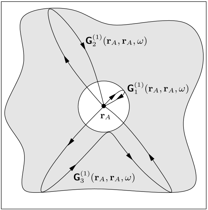
Figure 1: Schematic illustration of the interaction of the electromagnetic field with an atom at the center of an empty spherical cavity (at $\mathbf{r}_{A}$), embedded in a (isotropic) host medium of arbitrary size and shape. Simple examples of the three different kinds of processes are sketched. The corresponding Green tensors are $\mbox{{{G}}}_{1}^{(1)}(\mathbf{r}_{A},\mathbf{r}_{A},\omega)$, accounting for all scattering processes within the cavity, $\mbox{{{G}}}_{2}^{(1)}(\mathbf{r}_{A},\mathbf{r}_{A},\omega)$, describing (multiple) transmission through the cavity surface and accounting for all scattering processes in the host medium excluding reflection at the outer boundary of the cavity, and $\mbox{{{G}}}_{3}^{(1)}(\mathbf{r}_{A},\mathbf{r}_{A},\omega)$, including only the scattering processes involving (multiple) reflection at the outer boundary of the cavity.

where $\mbox{{{G}}}_{1}^{(1)}(\mathbf{r}_{A},\mathbf{r}_{A},\omega)$ accounts for (multiple) scattering at the inner surface of the cavity, $\mbox{{{G}}}_{2}^{(1)}(\mathbf{r}_{A},\mathbf{r}_{A},\omega)$ describes (multiple) transmission through the surface of the cavity without scattering at the outer surface of the cavity, and $\mbox{{{G}}}_{3}^{(1)}(\mathbf{r}_{A},\mathbf{r}_{A},\omega)$ is associated with (multiple) transmission through the surface of the cavity via scattering at the outer surface of the cavity. The decomposition is schematically illustrated in Fig. 1, showing a simple example each.

The term $\mbox{{{G}}}_{1}^{(1)}(\mathbf{r}_{A},\mathbf{r}_{A},\omega)$ in Eq. (III) is nothing but the scattering part of the Green tensor at the center of an empty sphere surrounded by an infinitely extended medium. In the case of a magnetoelectric medium of permittivity $\varepsilon(\omega)$ and permeability $\mu(\omega)$, it reads Li et al. (1994)

$$\mbox{{{G}}}_{1}^{(1)}(\mathbf{r}_{A},\mathbf{r}_{A},\omega)=\frac{i\omega}{6\pi c}\,C(\omega)\mbox{{{I}}},$$ (15)

where

$$C(\omega)=\frac{h_{1}^{(1)}(z_{0})\left[zh_{1}^{(1)}(z)\right]^{\prime}-\varepsilon(\omega)h_{1}^{(1)}(z)\left[z_{0}h_{1}^{(1)}(z_{0})\right]^{\prime}}{\varepsilon(\omega)h_{1}^{(1)}(z)\left[z_{0}j_{1}(z_{0})\right]^{\prime}-j_{1}(z_{0})\left[zh_{1}^{(1)}(z)\right]^{\prime}}$$ (16)

[$z_{0}$ $\!=$ $\!\omega R_{\mathrm{c}}/c$, $z$ $\!=$ $\!n(\omega)z_{0}$, $n(\omega)$ $\!=$ $\!\sqrt{\varepsilon(\omega)\mu(\omega)}\,$, the primes indicate derivatives], with $j_{1}(x)$ and $h_{1}^{(1)}(x)$, respectively, being the first spherical Bessel function and the first spherical Hankel function of the first kind,

$$j_{1}(x)=\frac{\sin(x)}{x^{2}}-\frac{\cos(x)}{x}\,,$$ (17)

$$h_{1}^{(1)}(x)=-\left(\frac{1}{x}+\frac{i}{x^{2}}\right)e^{ix}.$$ (18)

At this point it should already be mentioned that since the vdW potential depends on the Green tensor at all frequencies, an expansion for small $|\omega|R_{\mathrm{c}}/c$ of the form

$$C(\omega)=3\,\frac{\varepsilon(\omega)-1}{2\varepsilon(\omega)+1}\,\frac{c^{3}}{i\omega^{3}R_{\mathrm{c}}^{3}}\\ +\frac{9}{5}\,\frac{\varepsilon^{2}(\omega)[5\mu(\omega)-1]-3\,\varepsilon(\omega)-1}{[2\varepsilon(\omega)+1]^{2}}\,\frac{c}{i\omega R_{\mathrm{c}}}\\ +9\,\frac{\varepsilon(\omega)n^{3}(\omega)}{[2\varepsilon(\omega)+1]^{2}}-1+O\left(\frac{\omega R_{\mathrm{c}}}{c}\right)$$ (19)

and neglect of the term $O(\omega R_{\mathrm{c}}/c)$, as it is done in Ref. Ho et al. (2006) for the calculation of the decay rate of an excited atom, has to be applied with care (see Sec. IV.1.2).

Following the arguments given in Ref. Ho et al. (2006), the term $\mbox{{{G}}}_{2}^{(1)}(\mathbf{r}_{A},\mathbf{r}_{A},\omega)$ in Eq. (III) can always be written in the form

$$\mbox{{{G}}}_{2}^{(1)}(\mathbf{r}_{A},\mathbf{r}_{A},\omega)=f^{2}(\omega)\mbox{{{G}}}_{\mathrm{med}}^{(1)}(\mathbf{r}_{A},\mathbf{r}_{A},\omega),$$ (20)

where $\mbox{{{G}}}_{\mathrm{med}}^{(1)}(\mathbf{r}_{A},\mathbf{r}_{A},\omega)$ is the scattering part of the Green tensor of the undisturbed host medium (i.e., the medium without the cavity), and the global factor $f(\omega)$ can simply be determined from examining the Green tensor $\mbox{{{G}}}_{\mathrm{trans}}(\mathbf{r},\mathbf{r}_{A},\omega)$ which links a source at the center of the cavity with the transmitted field at a point $\mathbf{r}$ in the medium outside the cavity in the case of an infinitely extended medium. For a magnetoelectric medium, the Green tensor $\mbox{{{G}}}_{\mathrm{trans}}(\mathbf{r},\mathbf{r}_{A},\omega)$ reads Li et al. (1994)

$$\mbox{{{G}}}_{\mathrm{trans}}(\mathbf{r},\mathbf{r}_{A},\omega)=\frac{\mu(\omega)k}{4\pi}\,D(\omega)\\ \times\left[a(q)\mbox{{{I}}}-b(q)\mathbf{v}\mathbf{v}\right]e^{iq}$$ (21)

[$k$ $\!=$ $\!n(\omega)\omega/c$, $a(q)$ $\!=$ $\!1/q$ $\!+$ $\!i/q^{2}$ $\!-$ $\!1/q^{3}$, $b(q)$ $\!=$ $\!1/q$ $\!+$ $\!3i/q^{2}$ $\!-$ $\!3/q^{3}$, $q$ $\!=$ $\![n(\omega)\omega/c]|\mathbf{r}$ $\!-$ $\!\mathbf{r}_{A}|$, $\mathbf{v}$ $\!=$ $\!(\mathbf{r}$ $\!-$ $\!\mathbf{r}_{A})/(|\mathbf{r}$ $\!-$ $\!\mathbf{r}_{A}|)$], where

$$D(\omega)=\\ \frac{j_{1}(z_{0})\left[z_{0}h_{1}^{(1)}(z_{0})\right]^{\prime}-\left[z_{0}j_{1}(z_{0})\right]^{\prime}h_{1}^{(1)}(z_{0})}{\mu(\omega)\Bigl{\{}j_{1}(z_{0})\left[zh_{1}^{(1)}(z)\right]^{\prime}-\varepsilon(\omega)\left[z_{0}j_{1}(z_{0})\right]^{\prime}h_{1}^{(1)}(z)\Bigr{\}}}.$$ (22)

Comparing Eq. (21) with the Green tensor for an undisturbed, infinitely extended host medium,

$$\mbox{{{G}}}_{\mathrm{med}}^{(0)}(\mathbf{r},\mathbf{r}_{A},\omega)=\frac{\mu(\omega)k}{4\pi}\left[a(q)\mbox{{{I}}}-b(q)\mathbf{v}\mathbf{v}\right]e^{iq},$$ (23)

we see that the factor $f(\omega)$ is equal to $D(\omega)$,

$$f(\omega)=D(\omega).$$ (24)

Inspection of Eq. (22) for small $|\omega|R_{\mathrm{c}}/c$ shows that

$$D(\omega)=\frac{3\varepsilon(\omega)}{2\varepsilon(\omega)+1}+O\left(\frac{\omega R_{\mathrm{c}}}{c}\right).$$ (25)

Note that in leading order, the factor $D(\omega)$ is the same as that found for a purely electric system (cf. Ref. Ho et al. (2006)).

As shown in Ref. Ho et al. (2006), the term $\mbox{{{G}}}_{3}^{(1)}(\mathbf{r}_{A},\mathbf{r}_{A},\omega)$ in Eq. (III) behaves like $(\omega R_{\mathrm{c}}/c)^{3}$ for a sufficiently small cavity in a dielectric medium. The same asymptotic behavior is observed for magnetoelectric media, since, for sufficiently small $R_{\mathrm{c}}$, the leading-order contribution to $\mbox{{{G}}}_{3}^{(1)}(\mathbf{r}_{A},\mathbf{r}_{A},\omega)$ is determined by the electric properties. Recalling that in the real-cavity model the cavity radius is assumed to be small compared with the relevant atomic and medium wavelengths, $\mbox{{{G}}}_{3}^{(1)}(\mathbf{r}_{A},\mathbf{r}_{A},\omega)$ is in any case small compared with $\mbox{{{G}}}_{1}^{(1)}(\mathbf{r}_{A},\mathbf{r}_{A},\omega)$ and $\mbox{{{G}}}_{2}^{(1)}(\mathbf{r}_{A},\mathbf{r}_{A},\omega)$ and can thus be neglected, so that Eq. (III) [together with Eqs. (15), (20), and (24)] takes the form

$$\mbox{{{G}}}^{(1)}(\mathbf{r}_{A},\mathbf{r}_{A},\omega)=\frac{i\omega}{6\pi}\,C(\omega)\mbox{{{I}}}+D^{2}(\omega)\mbox{{{G}}}^{(1)}_{\mathrm{med}}(\mathbf{r}_{A},\mathbf{r}_{A},\omega).$$ (26)

So far we have concentrated on homogeneous host media of arbitrary shapes. An inhomogeneous medium can always be divided into a (small) homogeneous part that contains the cavity, such that the condition (12) is satisfied, and an inhomogeneous rest. Since all the scattering processes resulting from the inhomogeneous rest can be thought of as being taken into account by the scattering part of the Green tensor of the host medium, Eq. (26) still holds in this more general case. Note that a homogeneous medium of finite size can already be regarded as a special case of an inhomogeneous system. Hence, $\varepsilon(\omega)$ and $\mu(\omega)$, respectively, can be safely replaced by $\varepsilon_{A}(\omega)$ $\!\equiv$ $\!\varepsilon(\mathbf{r}_{A},\omega)$ and $\mu_{A}(\omega)$ $\!\equiv$ $\!\mu(\mathbf{r}_{A},\omega)$ in the equations given above [$C(\omega)\mapsto C_{A}(\omega)$, $D(\omega)\mapsto D_{A}(\omega)$].

Next we consider two atoms within a host medium of arbitrary size and shape, both located at the center of a small cavity, such that Eqs. (11) and (12) hold. In this case, there are two contributions to the Green tensor $\mbox{{{G}}}(\mathbf{r}_{A},\mathbf{r}_{B},\omega)$ that determines the electromagnetic field at the position $\mathbf{r}_{A}$ of atom $A$, originating at $\mathbf{r}_{B}$ where is atom $B$ located,

$$\mbox{{{G}}}(\mathbf{r}_{A},\mathbf{r}_{B},\omega)=\mbox{{{G}}}_{4}(\mathbf{r}_{A},\mathbf{r}_{B},\omega)+\mbox{{{G}}}_{5}(\mathbf{r}_{A},\mathbf{r}_{B},\omega).$$ (27)

Here, $\mbox{{{G}}}_{4}(\mathbf{r}_{A},\mathbf{r}_{B},\omega)$ accounts for (multiple) transmission through the cavity surfaces and (multiple) scattering at the inhomogeneities of the medium, excluding scattering at the outer boundaries of the cavities. As in the single-atom case, processes that involve (multiple) scattering at the outer surfaces of the cavities, described by $\mbox{{{G}}}_{5}(\mathbf{r}_{A},\mathbf{r}_{B},\omega)$, are neglected. The situation is sketched in Fig. 2.

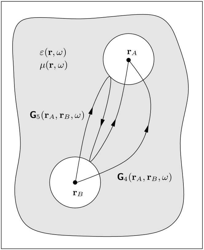
Figure 2: Schematic illustration of the interaction of the electromagnetic field with two atoms, each placed in a spherical cavity, surrounded by a host medium of arbitrary size and shape. The relevant Green tensors $\mbox{{{G}}}_{4}(\mathbf{r}_{A},\mathbf{r}_{A},\omega)$ and $\mbox{{{G}}}_{5}(\mathbf{r}_{A},\mathbf{r}_{A},\omega)$ account for (multiple) transmission through the cavity surfaces and (multiple) scattering at the inhomogeneities of the host medium including (multiple) scattering at the outer boundaries of the cavities, respectively.

By means of the same arguments as in the single-atom case, we find a global factor that accounts for transmission through the surfaces of the cavities such that the field at $\mathbf{r}$ outside the cavities which results from $\mathbf{r}_{B}$, may be calculated from $D_{B}(\omega)\mbox{{{G}}}_{\mathrm{med}}(\mathbf{r},\mathbf{r}_{B},\omega)$. Due to the property $\mbox{{{G}}}(\mathbf{r},\mathbf{r^{\prime}},\omega)$ $\!=$ $\!\mbox{{{G}}}^{\mathsf{T}}(\mathbf{r^{\prime}},\mathbf{r},\omega)$ of the Green tensor, we also find that $D_{A}(\omega)\mbox{{{G}}}_{\mathrm{med}}(\mathbf{r}_{A},\mathbf{r},\omega)$ determines the electromagnetic field at point $\mathbf{r}_{A}$ originating at point $\mathbf{r}$ outside the cavities. We may thus write $\mbox{{{G}}}(\mathbf{r}_{A},\mathbf{r}_{B},\omega)$ in the form

$$\mbox{{{G}}}(\mathbf{r}_{A},\mathbf{r}_{B},\omega)=D_{A}(\omega)\mbox{{{G}}}_{\mathrm{med}}(\mathbf{r}_{A},\mathbf{r}_{B},\omega)D_{B}(\omega).$$ (28)

IV Local-field corrected van der Waals interaction

IV.1 Single atom within an arbitrary magnetoelectric medium

Within the framework of the real-cavity model, local-field corrected vdW interactions can now be calculated by combining the formulas given in Sec. II and III, where we again begin with the case of a single guest atom. We substitute $\mbox{{{G}}}{{}^{(1)}}(\mathbf{r}_{A},\mathbf{r}_{A},\omega)$ as given by Eq. (26) into Eq. (1) to obtain

$$U(\mathbf{r}_{A})=U_{1}(\mathbf{r}_{A})+U_{2}(\mathbf{r}_{A}),$$ (29)

where

$$U_{1}(\mathbf{r}_{A})= \,-\frac{\hbar\mu_{0}}{12\pi^{2}c}\int_{0}^{\infty}\mathrm{d}u\,u^{3}C_{A}(iu)\mathrm{Tr}\,\bm{\alpha}_{A}(iu),$$ (30)

$$U_{2}(\mathbf{r}_{A})= \,\frac{\hbar\mu_{0}}{2\pi}\int_{0}^{\infty}\mathrm{d}u\,u^{2}D_{A}^{2}(iu)$$

$$\times\mathrm{Tr}\!\left[\bm{\alpha}_{A}(iu)\!\cdot\!\mbox{{{G}}}_{\mathrm{med}}^{(1)}(\mathbf{r}_{A},\mathbf{r}_{A},iu)\right]$$ (31)

[$C_{A}(iu)$ and $D_{A}(iu)$ according to Eqs. (16) and (22), respectively].

IV.1.1 Linear approximation

In order to make contact with a microscopic description and provide a deeper insight into the validity of the real-cavity model, let us first restrict our attention to to weakly polarizable and/or magnetizable host material so that the linear approximation applies. In this case, we may regard $\varepsilon(\mathbf{r},\omega)$ and $\mu(\mathbf{r},\omega)$ as being only slightly perturbed from their free-space values,

$$\varepsilon(\mathbf{r},\omega)= \,1+\chi(\mathbf{r},\omega),$$ (32)

$$\mu(\mathbf{r},\omega)= \,1+\zeta(\mathbf{r},\omega)$$ (33)

[$|\chi(\mathbf{r},\omega)|$ $\!\ll$ $\!1$, $|\zeta(\mathbf{r},\omega)|$ $\!\ll$ $\!1$], and approximate $U_{1}(\mathbf{r}_{A})$, Eq. (30), by

$$U_{1}(\mathbf{r}_{A})=-\frac{\hbar\mu_{0}}{4\pi^{2}c}\int_{0}^{\infty}\mathrm{d}u\,u^{3}\alpha_{A}(iu)e^{-2uR_{\mathrm{c}}/c}\\ \times\left[\left(\frac{c^{3}}{u^{3}R_{\mathrm{c}}^{3}}+\frac{2c^{2}}{u^{2}R_{\mathrm{c}}^{2}}+\frac{c}{uR_{\mathrm{c}}}+\frac{1}{2}\right)\chi(\mathbf{r}_{A},iu)\right.\\ \left.-\left(\frac{c}{uR_{\mathrm{c}}}+\frac{1}{2}\right)\zeta(\mathbf{r}_{A},iu)\right],$$ (34)

where we have assumed a spherically symmetric atom. By straightforward calculation, one can then show that

$$U_{1}(\mathbf{r}_{A})=\rho(\mathbf{r}_{A})\int_{|\mathbf{s}-\mathbf{r}_{A}|\geq R_{\mathbf{c}}}\mathrm{d}^{3}s\,U(\mathbf{r}_{A},\mathbf{s}),$$ (35)

where $\rho(\mathbf{r})$ is the number density of the medium atoms,

$$U(\mathbf{r}_{A},\mathbf{s})=U^{\mathrm{el}}(\mathbf{r}_{A},\mathbf{s})+U^{\mathrm{mag}}(\mathbf{r}_{A},\mathbf{s})$$ (36)

($\mathbf{r}_{A}$ $\!\neq$ $\!\mathbf{s}$) is the vdW potential of two unpolarized, neutral (ground state) atoms in free space, with the electric and magnetic parts being given by Buhmann and Welsch (2006a)

$$U^{\mathrm{el}}(\mathbf{r}_{A},\mathbf{r})=-\frac{\hbar\mu_{0}^{2}}{2\pi}\int_{0}^{\infty}\mathrm{d}u\,u^{4}\alpha_{A}(iu)\alpha(iu)\\ \times\mathrm{Tr}[\mbox{{{G}}}_{\mathrm{free}}(\mathbf{r}_{A},\mathbf{r},iu)\!\cdot\!\mbox{{{G}}}_{\mathrm{free}}(\mathbf{r},\mathbf{r}_{A},iu)]\\ =-\frac{\hbar}{32\pi^{3}\varepsilon_{0}^{2}l^{6}}\int_{0}^{\infty}\mathrm{d}u\,\alpha_{A}(iu)\alpha(iu)g(ul/c)$$ (37)

and

$$U^{\mathrm{mag}}(\mathbf{r}_{A},\mathbf{r})=-\frac{\hbar\mu_{0}^{2}}{2\pi}\int_{0}^{\infty}\mathrm{d}u\,u^{2}\alpha_{A}(iu)\beta(iu)\\ \times\mathrm{Tr}\!\left\{\left[\mbox{{{G}}}_{\mathrm{free}}(\mathbf{r}_{A},\mathbf{s},iu)\!\times\!\overleftarrow{\bm{\nabla}}_{\mathbf{s}}\right]\!\cdot\!\bm{\nabla}_{\mathbf{s}}\!\times\!\mbox{{{G}}}_{\mathrm{free}}(\mathbf{s},\mathbf{r}_{A},iu)\right\}_{\mathbf{s}=\mathbf{r}}\\ =\frac{\hbar\mu_{0}^{2}}{32\pi^{3}l^{4}}\int_{0}^{\infty}\mathrm{d}u\,u^{2}\alpha_{A}(iu)\beta(iu)h(ul/c)$$ (38)

[$g(x)=2e^{-2x}(3+6x+5x^{2}+2x^{3}+x^{4})$, $h(x)=2e^{-2x}(1+2x+x^{2})$, $l=|\mathbf{r}_{A}-\mathbf{r}|$; $\mbox{{{G}}}_{\mathrm{free}}(\mathbf{r},\mathbf{s},iu)$, free-space Green tensor; $\alpha(iu)$, polarizability; $\beta(iu)$, magnetizability of the medium atoms], where we have made the identifications

$$\chi(\mathbf{r},\omega)=\varepsilon_{0}^{-1}\rho(\mathbf{r})\alpha(\omega),$$ (39)

$$\zeta(\mathbf{r},\omega)=\mu_{0}\rho(\mathbf{r})\beta(iu).$$ (40)

To find the linear approximation to $U_{2}(\mathbf{r}_{A})$, Eq. (IV.1), let us first consider

$$\mbox{{{G}}}_{\mathrm{med}}^{(1)}(\mathbf{r}_{A},\mathbf{r}_{A},\omega)=\mbox{{{G}}}_{\mathrm{med}}(\mathbf{r}_{A},\mathbf{r}_{A},\omega)-\mbox{{{G}}}_{\mathrm{med}}^{(0)}(\mathbf{r}_{A},\mathbf{r}_{A},\omega).$$ (41)

Applying the linear Born expansion (see, e.g., Ref. Ho et al. (2006))

$$\mbox{{{G}}}(\mathbf{r},\mathbf{r}^{\prime},\omega)=\mbox{{{G}}}_{\mathrm{free}}(\mathbf{r},\mathbf{r}^{\prime},\omega)+\Delta\mbox{{{G}}}(\mathbf{r},\mathbf{r}^{\prime},\omega)$$ (42)

$$\Delta\mbox{{{G}}}(\mathbf{r},\mathbf{r}^{\prime},\omega)=\Delta\mbox{{{G}}}^{\mathrm{el}}(\mathbf{r},\mathbf{r}^{\prime},\omega)+\Delta\mbox{{{G}}}^{\mathrm{mag}}(\mathbf{r},\mathbf{r}^{\prime},\omega),$$ (43)

with

$$\Delta\mbox{{{G}}}^{\mathrm{el}}(\mathbf{r},\mathbf{r}^{\prime},\omega)=\frac{\omega^{2}}{c^{2}}\int\mathrm{d}^{3}s\,\chi(\mathbf{s},\omega)\\ \times\mbox{{{G}}}_{\mathrm{free}}(\mathbf{r},\mathbf{s},\omega)\!\cdot\!\mbox{{{G}}}_{\mathrm{free}}(\mathbf{s},\mathbf{r}^{\prime},\omega),$$ (44)

$$\Delta\mbox{{{G}}}^{\mathrm{mag}}(\mathbf{r},\mathbf{r}^{\prime},\omega)=-\int\mathrm{d}^{3}s\,\zeta(\mathbf{s},\omega)\\ \times\left[\mbox{{{G}}}_{\mathrm{free}}(\mathbf{r},\mathbf{s},\omega)\!\times\!\overleftarrow{\bm{\nabla}}_{s}\right]\!\cdot\!\bm{\nabla}_{s}\!\times\!\mbox{{{G}}}_{\mathrm{free}}(\mathbf{s},\mathbf{r}^{\prime},\omega)$$ (45)

to the calculation of the Green functions $\mbox{{{G}}}_{\mathrm{med}}(\mathbf{r}_{A},\mathbf{r}_{A},\omega)$ and $\mbox{{{G}}}_{\mathrm{med}}^{(0)}(\mathbf{r}_{A},\mathbf{r}_{A},\omega)$ in Eq. (41), we derive

$$\mbox{{{G}}}^{(1)}_{\mathrm{med}}(\mathbf{r}_{A},\mathbf{r}_{A},\omega)=\\ \frac{\omega^{2}}{c^{2}}\int_{\mathrm{V}}\mathrm{d}^{3}s\,\chi(\mathbf{s},\omega)\mbox{{{G}}}_{\mathrm{free}}(\mathbf{r}_{A},\mathbf{s},\omega)\!\cdot\!\mbox{{{G}}}_{\mathrm{free}}(\mathbf{s},\mathbf{r}_{A},\omega)\\ -\int_{\mathrm{V}}\mathrm{d}^{3}s\,\zeta(\mathbf{s},\omega)\left[\mbox{{{G}}}_{\mathrm{free}}(\mathbf{r},\mathbf{s},\omega)\!\times\!\overleftarrow{\bm{\nabla}}_{s}\right]\!\cdot\!\bm{\nabla}_{s}\!\times\!\mbox{{{G}}}_{\mathrm{free}}(\mathbf{s},\mathbf{r}^{\prime},\omega)\\ -\frac{\omega^{2}\chi(\mathbf{r}_{A},\omega)}{c^{2}}\int\mathrm{d}^{3}s\,\mbox{{{G}}}_{\mathrm{free}}(\mathbf{r}_{A},\mathbf{s},\omega)\!\cdot\!\mbox{{{G}}}_{\mathrm{free}}(\mathbf{s},\mathbf{r}_{A},\omega)\\ +\,\zeta(\mathbf{r}_{A},\omega)\int\mathrm{d}^{3}s\left[\mbox{{{G}}}_{\mathrm{free}}(\mathbf{r},\mathbf{s},\omega)\!\times\!\overleftarrow{\bm{\nabla}}_{s}\right]\!\cdot\!\bm{\nabla}_{s}\!\times\!\mbox{{{G}}}_{\mathrm{free}}(\mathbf{s},\mathbf{r}^{\prime},\omega)$$ (46)

($V$, volume of the unperturbed host medium). Equation (46) reveals that, in contrast to $D_{A}(\omega)$, $\mbox{{{G}}}_{\mathrm{med}}^{(1)}(\mathbf{r}_{A},\mathbf{r}_{A},\omega)$ has no zero-order contribution with respect to $\chi(\mathbf{r},\omega)$ and $\zeta(\mathbf{r},\omega)$. Thus, the linear approximation to $U_{2}(\mathbf{r}_{A})$ can be obtained by substituting Eq. (46) into Eq. (IV.1), letting $D_{A}(\omega)$ $\!=$ $\!1$, and applying Eqs. (39) and (40), which results in

$$U_{2}(\mathbf{r}_{A})= \int_{\mathrm{V}}\mathrm{d}^{3}s\,\rho(\mathbf{s})U(\mathbf{r}_{A},\mathbf{s})$$

$$\;-\rho(\mathbf{r}_{A})\int\mathrm{d}^{3}s\,U(\mathbf{r}_{A},\mathbf{s}).$$ (47)

As expected, the overall potential in linear approximation is simply

$$U(\mathbf{r}_{A}) =U_{1}(\mathbf{r}_{A})+U_{2}(\mathbf{r}_{A})$$

$$=\int_{\mathrm{V^{\prime}}}\mathrm{d}^{3}s\,\rho(\mathbf{s})U(\mathbf{r}_{A},\mathbf{s})$$ (48)

($\mathrm{V^{\prime}}$, volume of the host medium excluding the volume of the cavity), where we have recalled Eq. (12).

The results found in linear approximation, particularly Eq. (IV.1.1), indicate that $R_{\mathrm{c}}$ can indeed be identified with an average inter-atomic distance. Hence, the real-cavity model can be regarded as being valid down to a microscopic scale. Since $U_{1}(\mathbf{r}_{A})$ can be described as the sum of the vdW interactions between the guest atom and all the atoms in an infinitely extended homogeneous medium, it does not lead to a force but to a more or less significant shift of the overall potential, which is dominated by the interaction of the guest atom with the neighboring host atoms. Note that we have demonstrated these results up to linear order in $\chi(\mathbf{r},\omega)$ and $\zeta(\mathbf{r},\omega)$. In principle, a generalization beyond the linear Born expansion should be possible, although associated with extensive calculations. In this case many-atom vdW interactions have to be taken into account.

IV.1.2 Beyond the linear approximation

Let us return to the integrals in Eqs. (30) and (IV.1). To find the local-field correction, one has in fact to consider the leading-order terms in $R_{\mathrm{c}}$ after the frequency integrals have been performed. However, since $\varepsilon_{A}(\omega)-1$, $\mu_{A}(\omega)-1$, and $\alpha_{A}(\omega)$ provide cut-off functions for the $u$-integrals [giving their main contribution for $u\lesssim\omega_{\max}$, with $\omega_{\max}$ being the maximum of all relevant atomic and medium resonance frequencies] and assuming that $\omega_{\max}R_{\mathrm{c}}/c\ll 1$, we may expand $C_{A}(iu)$ and $D_{A}(iu)$ in the integrands, keep the leading-order terms in $uR_{\mathrm{c}}/c$, and integrate over $u$ afterwards. This procedure can be justified by the good convergence behavior in the asymptotic limit of small $R_{\mathrm{c}}$, which we have confirmed numerically.

Thus, using Eq. (19), we can write $U_{1}(\mathbf{r}_{A})$, Eq. (30), in the form

$$U_{1}(\mathbf{r}_{A})=-\frac{\hbar\mu_{0}}{4\pi^{2}}\int_{0}^{\infty}\mathrm{d}u\left[\frac{\varepsilon_{A}(iu)-1}{2\varepsilon_{A}(iu)+1}\,\frac{c^{2}}{R_{\mathrm{c}}^{3}}\right.\\ \left.+\,3\,\frac{\varepsilon_{A}^{2}(iu)\left[1-5\mu_{A}(iu)\right]+3\varepsilon_{A}(iu)+1}{5\left[2\varepsilon_{A}(iu)+1\right]^{2}}\,\frac{u^{2}}{R_{\mathrm{c}}}\right]\\ \times\mathrm{Tr}\,\bm{\alpha}_{A}(iu).$$ (49)

As already mentioned, $U_{1}(\mathbf{r}_{A})$ can be ignored if one is only interested in the force on the atom (see also App. A). Similarly, using Eq. (25), we can write $U_{2}(\mathbf{r}_{A})$, Eq. (IV.1), as

$$U_{2}(\mathbf{r}_{A})=\frac{\hbar\mu_{0}}{2\pi}\int_{0}^{\infty}\mathrm{d}uu^{2}\left[\frac{3\varepsilon_{A}(iu)}{2\varepsilon_{A}(iu)+1}\right]^{2}\\ \times\mathrm{Tr}\left[\bm{\alpha}_{A}(iu)\!\cdot\!\mbox{{{G}}}_{\mathrm{med}}^{(1)}(\mathbf{r}_{A},\mathbf{r}_{A},iu)\right].$$ (50)

With Eq. (6) and the condition (12), one obtains

$$\mathbf{F}(\mathbf{r}_{A})= -\frac{\hbar\mu_{0}}{2\pi}\int_{0}^{\infty}\mathrm{d}uu^{2}\left[\frac{3\varepsilon_{A}(iu)}{2\varepsilon_{A}(iu)+1}\right]^{2}$$

$$\times\bm{\nabla}_{\!\!A}\mathrm{Tr}\left[\bm{\alpha}_{A}(iu)\cdot\mbox{{{G}}}_{\mathrm{med}}^{(1)}(\mathbf{r}_{A},\mathbf{r}_{A},iu)\right]$$ (51)

for the local-field corrected vdW force on a ground-state atom within an arbitrary magnetoelectric system.

In the limit of the atom being embedded in a very dilute medium, $\varepsilon_{A}(iu)-1$ $\!\ll$ $\!1$ and $\mu_{A}(iu)-1$ $\!\ll$ $\!1$, the local-field correction becomes negligible and Eqs. (49)–(IV.1.2) approach the uncorrected result [Eqs. (1) and (6)], as expected. As a note of caution, we remark that, quite contrary, in the limit $R_{\mathrm{c}}$ $\!\to$ $\!0$, the local-field corrected result does not approach the uncorrected one, which might be obtained when the atom is thought of as not being placed in an empty free-space region, but being placed in a region which is continuously filled with medium. This is due to the fact that there is no continuous $R_{\mathrm{c}}$ $\!\to$ $\!0$ transition from the corrected setup (an atom inside an empty free-space cavity surrounded by a medium) and the uncorrected one (an atom inside the medium): Even as the cavity radius is made smaller and smaller, the atom will always remain inside a free-space region.

Equation (IV.1.2) shows that, in comparison to the uncorrected vdW force (6), the contributions to the $u$-integral are enhanced by a factor between $1$ and $9/4$ owing to the local-field correction. Note that the enhancement factor varies with $u$ and the uncorrected contributions can in general (in particular, for magnetoelectric media) have different signs for different values of $u$. Hence, the local-field corrected vdW force can be enhanced or reduced. For example, for (purely electric) media important in biological applications, local-field corrections can lead to enhancements by factors of $2.22$ [for water with $\varepsilon(0)\approx 80$] or $1.86\ldots 2.19$ (for typical plasma membrane compositions with $\varepsilon(0)\approx 5\ldots 40$ Nir (1976)).

IV.2 Two or more atoms within an arbitrary magnetoelectric medium

Using Eqs. (7) and (28), the local-field corrected two-atom vdW potential reads

$$U(\mathbf{r}_{A},\mathbf{r}_{B})=-\frac{\hbar\mu_{0}^{2}}{2\pi}\int_{0}^{\infty}\mathrm{d}uu^{4}D_{A}(iu)D_{B}(iu)\\ \times\mathrm{Tr}[\bm{\alpha}_{A}(iu)\!\cdot\!\mbox{{{G}}}_{\mathrm{med}}(\mathbf{r}_{A},\mathbf{r}_{B},iu)\!\cdot\!\bm{\alpha}_{B}(iu)\!\cdot\!\mbox{{{G}}}_{\mathrm{med}}(\mathbf{r}_{B},\mathbf{r}_{A},iu)].\\[-8.61108pt]$$ (52)

In analogy to Sec. IV.1.2, we may expand the coefficients $D_{A}(iu)$ and $D_{B}(iu)$ to leading order in $uR_{\mathrm{c}}/c$, as given by Eq. (25), and integrate afterwards. Hence, Eq. (52) leads to

$$U(\mathbf{r_{A}},\mathbf{r_{B}})=-\frac{\hbar\mu_{0}^{2}}{2\pi}\\ \times\int_{0}^{\infty}\mathrm{d}uu^{4}\left[\frac{3\varepsilon_{A}(iu)}{2\varepsilon_{A}(iu)+1}\right]^{2}\left[\frac{3\varepsilon_{B}(iu)}{2\varepsilon_{B}(iu)+1}\right]^{2}\\ \times\!\mathrm{Tr}[\bm{\alpha}_{A}(iu)\!\cdot\!\mbox{{{G}}}_{\mathrm{med}}(\mathbf{r}_{A},\mathbf{r}_{B},iu)\!\cdot\!\bm{\alpha}_{B}(iu)\!\cdot\!\mbox{{{G}}}_{\mathrm{med}}(\mathbf{r}_{B},\mathbf{r}_{A},iu)].\\[-8.61108pt]$$ (53)

In comparison to the uncorrected potential (7), the contributions to the $u$-integral are enhanced by a factor which varies between $1$ and $81/16$, so that altogether an enhancement or an reduction of the local-field corrected two-atom force may be observed (recall the remark at the end of Sec. IV.1.2).

Equation (53) can easily be extended to the mutual interaction of $N$ atoms. Substituting Eqs. (25) and (28) into Eq. (9), one finds that, for isotropic atoms, the local-field corrected $N$-atom potential is given by

$$U(\mathbf{r}_{1},\dots,\mathbf{r}_{N})=\frac{(-1)^{N-1}\hbar\mu_{0}^{N}}{(1+\delta_{2N})\pi}\int_{0}^{\infty}\mathrm{d}u\,u^{2N}\\ \times\left[\frac{3\varepsilon_{1}(iu)}{2\varepsilon_{1}(iu)+1}\right]^{2}\cdots\left[\frac{3\varepsilon_{N}(iu)}{2\varepsilon_{N}(iu)+1}\right]^{2}\alpha_{1}(iu)\cdots\alpha_{N}(iu)\\ \times\mathrm{Tr}\left[\mbox{{{G}}}_{\mathrm{med}}(\mathbf{r}_{1},\mathbf{r}_{2},iu)\cdots\mbox{{{G}}}_{\mathrm{med}}(\mathbf{r}_{N},\mathbf{r}_{1},iu)\right].$$ (54)

IV.3 Example: Two atoms within a bulk magnetoelectric medium

As a simple example, let us consider two isotropic ground-state atoms embedded in magnetoelectric bulk material characterized by $\varepsilon(\omega)$ and $\mu(\omega)$. Substituting Eq. (23) into Eq. (53), we obtain

$$U(\mathbf{r}_{A},\mathbf{r}_{B})=-\frac{\hbar}{16\pi^{3}\varepsilon^{2}_{0}l^{6}}\int_{0}^{\infty}\mathrm{d}u\,\frac{\alpha_{A}(iu)\alpha_{B}(iu)}{\varepsilon^{2}(iu)}\\ \times\left[\frac{3\varepsilon(iu)}{2\varepsilon(iu)+1}\right]^{4}\left\{3+6n(iu)ul/c+5[n(iu)ul/c]^{2}\right.\\ \left.+2[n(iu)ul/c]^{3}+[n(iu)ul/c]^{4}\right\}e^{-2n(iu)ul/c},$$ (55)

where $l=$ $\!|\mathbf{r}_{A}$ $\!-$ $\!\mathbf{r}_{B}|$. In the retarded limit, $l$ $\!\gg$ $\!c/\omega_{\min}$ (with $\omega_{\min}$ denoting the minimum of all the relevant atomic and medium resonance frequencies), the main contributions to the $u$-integral come from the range where

$$\alpha_{A(B)}(iu)\simeq\alpha_{A(B)}(0),\;\varepsilon(iu)\simeq\varepsilon(0),\;\mu(iu)\simeq\mu(0).$$ (56)

With this inserted, Eq. (55) simplifies to

$$U(\mathbf{r}_{A},\mathbf{r}_{B})=-\frac{C_{\mathrm{r}}}{l^{7}},$$ (57)

where

$$C_{\mathrm{r}}=\frac{23\hbar c}{64\pi^{3}\varepsilon_{0}^{2}}\frac{\alpha_{A}(0)\alpha_{B}(0)}{n(0)\varepsilon^{2}(0)}\left[\frac{3\varepsilon(0)}{2\varepsilon(0)+1}\right]^{4}.$$ (58)

In the non-retarded limit, $l$ $\!\ll$ $\!c/n(0)\omega_{\max}$, we may set $e^{-2n(iu)ul/c}$ $\!\simeq$ $\!1$ and approximate the term in the curly brackets by $3$. In this way, Eq. (55) reduces to

$$U(\mathbf{r}_{A},\mathbf{r}_{B})=-\frac{C_{\mathrm{nr}}}{l^{6}},$$ (59)

where

$$C_{\mathrm{nr}}=\frac{3\hbar}{16\pi^{3}\varepsilon_{0}^{2}}\int_{0}^{\infty}\mathrm{d}u\,\frac{\alpha_{A}(iu)\alpha_{B}(iu)}{\varepsilon^{2}(iu)}\left[\frac{3\varepsilon(iu)}{2\varepsilon(iu)+1}\right]^{4}.$$ (60)

Equations (57) and (59) generalize the well-known results for the uncorrected mutual vdW interaction of two atoms in bulk material Dzyaloshinskii et al. (1961). We see that the local-field corrected potential follows the usual $l^{-7}$ and $l^{-6}$ dependence in the retarded and non-retarded limits, respectively. However, due to the influence of the local-field correction, the potential/force can be noticeably enhanced in dense media.

V Summary

In this paper, we have studied the local-field corrected vdW interaction of ground-state atoms embedded in a finite magnetoelectric medium of arbitrary size and shape. We have started from the familiar expressions for the one- and many-atom vdW potentials in leading-order perturbation theory, given in terms of the associated (classical) Green tensors and the atomic polarizabilities. Employing the real-cavity model for the local-field correction and using the methods developed in Ref. Ho et al. (2006), we have derived general expressions for the required local-field corrected Green tensors. Using these results, we have obtained geometry-independent, general formulas for the local-field corrected one- and many-atom (ground-state) vdW potentials and the corresponding forces.

The derivation is based on the assumption that the radius of the free-space cavity, in which a guest atom is thought of as being located and which is a measure of the average distance of the guest atom from the surrounding host atoms, is small compared to the other characteristic lengths of the problem. That is to say, it should be small compared to the distance of a guest atom from surfaces of discontinuity of the host medium, the distances between the guest atoms in the case of many-atom interactions, and the wavelengths associated with the electromagnetic response of the guest atoms and the host medium. It should be pointed out that under these conditions the forces do not explicitly depend on the cavity radius.

We have found that the local-field correction leads to a position-independent shift of the single-atom potential, while at the same time enhancing the contributions to the position-dependent part by a frequency-dependent factor that may vary between $1$ and $9/4$. The frequency-dependent contributions to the two-atom potential, on the other hand, are enhanced by a factor between $1$ and $81/16$ owing to the local-field correction. The contributions to the general $N$-atom potential are enhanced accordingly. In all cases, the respective vdW force can be enhanced or reduced.

As a simple example, we have calculated the mutual vdW potential of two ground-state atoms placed within a magnetoelectric bulk medium. The result shows that the potential follows the well-known asymptotic $l^{-7}$ and $l^{-6}$ power laws in the retarded and non-retarded regimes, respectively, where the local-field correction leads to an enhancement of the associated proportionality constants.

We conclude by noting that, besides vdW interaction and spontaneous decay, the local-field corrected Green tensors obtained can also be used to account for the effects of the local field in a number of important processes (e.g., fluorescence, light scattering, energy transfer, etc.). Evidently, one can expect that these processes are affected by local-field corrections in a similar way as found here.

Appendix A Atom inside a free-space cavity

In Sec. IV, we have encountered the potential term $U_{1}(\mathbf{r}_{A})$, Eq. (30), which is equal to the potential of an atom at the center of a free-space cavity embedded in a bulk medium of permittivity $\varepsilon_{A}(\omega)$ and permeability $\mu_{A}(\omega)$. More generally, the potential of an atom at a small displacement $\overline{\mathbf{r}}_{A}$ from the center of the cavity is given by Eq. (1) with the Green tensor Li et al. (1994)

$$\mbox{{{G}}}^{(1)}(\mathbf{r}_{A},\mathbf{r}_{A},\omega)=\frac{i\omega}{4\pi c}\sum_{l=1}^{\infty}(2l+1)\Bigl{\{}C^{E}_{l}(\omega)l(l+1)\frac{j^{2}_{l}(\xi_{A})}{\xi^{2}_{A}}\\ \times\,\mathbf{e}_{r}\mathbf{e}_{r}+\frac{1}{2}\left[C_{l}^{E}(\omega)\frac{[\xi_{A}j_{l}(\xi_{A})]^{\prime 2}}{\xi^{2}_{A}}+C^{M}_{l}(\omega)j^{2}_{l}(\xi_{A})\right]\\ \times(\mathbf{e}_{\theta}\mathbf{e}_{\theta}+\mathbf{e}_{\phi}\mathbf{e}_{\phi})\Bigr{\}}.$$ (61)

($\mathbf{e}_{r}$, $\mathbf{e}_{\theta}$, $\mathbf{e}_{\phi}$, spherical unit vectors associated with $\overline{\mathbf{r}}_{A}$; $\xi_{A}$ $\!=$ $\!\omega\overline{r}_{A}/c$). Here $C^{E}_{l}$ is given by Eq. (16), with the subscript $1\rightarrow l$, and $C^{M}_{l}$ $\!=$ $\!C^{E}_{l}[\varepsilon\leftrightarrow\mu]$. From

$$j_{l}(\xi_{A})\simeq\frac{\xi^{l}_{A}}{(2l+1)!!}\quad\mbox{for }\xi_{A}\ll 1,$$ (62)

we have

$$\mbox{{{G}}}^{(1)}(\mathbf{r}_{A},\mathbf{r}_{A},\omega)=\frac{i\omega}{4\pi c}\sum_{l=1}^{\infty}(2l+1)C_{l}^{E}(\omega)\biggl{[}\frac{\xi^{l-1}_{A}}{(2l+1)!!}\biggr{]}^{2}\\ \times\bigl{[}l(l+1)\mathbf{e}_{r}\mathbf{e}_{r}+{\textstyle\frac{1}{2}}(l+1)^{2}(\mathbf{e}_{\theta}\mathbf{e}_{\theta}+\mathbf{e}_{\phi}\mathbf{e}_{\phi})\bigr{]}$$ (63)

for the small $\xi_{A}$ expansion of the Green tensor. As seen, in the limit $\xi_{A}\rightarrow 0$, only the $l$ $\!=$ $\!1$ term survives, leading to the potential (30). The force on an atom close to the cavity center is determined by the derivative of the Green function with respect to $\overline{r}_{A}$. Therefore, for small displacements of the atom from the cavity center, it is given by the $l$ $\!=$ $\!2$ term in the above expansion, and we find the linear force

$$\mathbf{F}({\mathbf{r}}_{A})=-\mathbf{e}_{r}\frac{\partial}{\partial\overline{r}_{A}}\,U({\mathbf{r}}_{A})=K\overline{\mathbf{r}}_{A}$$ (64)

with

$$K=-\frac{\hbar}{12\pi^{2}\varepsilon_{0}c^{5}}\int_{0}^{\infty}\mathrm{d}u\,u^{5}\alpha_{A}(iu)C_{2}^{E}(iu),$$ (65)

[recall Eq. (16)], which vanishes at the cavity center. For small cavity radii Eq. (65) reduces to

$$K=\frac{\hbar}{12\pi^{2}\varepsilon_{0}c^{5}}\int_{0}^{\infty}\mathrm{d}u\,u^{5}\alpha_{A}(iu)\left\{90\,\frac{\varepsilon(iu)-1}{3\varepsilon(iu)+2}\,\frac{c^{5}}{u^{5}R_{\mathrm{c}}^{5}}\right.\\ -\left.\frac{75}{7}\,\frac{\varepsilon^{2}(iu)[7\mu(iu)+3]-6\varepsilon(iu)-4}{[3\varepsilon(iu)+2]^{2}}\,\frac{c^{3}}{u^{3}R_{\mathrm{c}}^{3}}\right\},$$ (66)

leading to a force pointing away from the center of the cavity (corresponding to an unstable equilibrium) for materials with purely dielectric properties and to a harmonic force for purely magnetic materials.

References

- Casimir and Polder (1948) H. B. G. Casimir and D. Polder, Phys. Rev. 73, 360 (1948).
- McLachlan (1963) A. D. McLachlan, Proc. R. Soc. London, Ser. A 271, 387 (1963).
- McLachlan (1964) A. D. McLachlan, Mol. Phys. 7, 381 (1964).
- Agarwal (1975) G. S. Agarwal, Phys. Rev. A 11, 243 (1975).
- Mahanty and Ninham (1973) J. Mahanty and B. W. Ninham, J. Phys. A: Math. Gen. 6, 1140 (1973).
- Mahanty and Ninham (1976) J. Mahanty and B. W. Ninham, Dispersion Forces (Academic, London, 1976).
- Wylie and Sipe (1984) J. M. Wylie and J. E. Sipe, Phys. Rev. A 30, 1185 (1984).
- Buhmann et al. (2004) S. Y. Buhmann, L. Knöll, D.-G. Welsch, and D. T. Ho, Phys. Rev. A 70, 052177 (2004).
- Safari et al. (2006) H. Safari, S. Y. Buhmann, D.-G. Welsch, and D. T. Ho, Phys. Rev. A 74, 042101 (2006).
- Buhmann and Welsch (2006a) S. Y. Buhmann and D.-G. Welsch, Prog. Quant. Electron. 31, 51 (2006).
- Ho et al. (1998) D. T. Ho, L. Knöll, and D.-G. Welsch, Phys. Rev. A 57, 3931 (1998).
- (12) L. Knöll, S. Scheel, and D.-G. Welsch, in Coherence and Statistics of Photons and Atoms, edited by J. Peřina, p. 1 (Wiley, New York, 2001).
- Ho et al. (2003) D. T. Ho, S. Y. Buhmann, L. Knöll, D.-G. Welsch, S. Scheel, and J. Kästel, Phys. Rev. A 68, 043816 (2003).
- Onsager (1936) L. Onsager, J. Am. Chem. Soc. 58, 1486 (1936).
- Scheel et al. (1999) S. Scheel, L. Knöll, and D.-G. Welsch, Phys. Rev. A 60, 4094 (1999).
- Tomaš (2001) M. S. Tomaš, Phys. Rev. A 63, 053811 (2001).
- Ho et al. (2006) D. T. Ho, S. Y. Buhmann, and D.-G. Welsch, Phys. Rev. A 74, 023803 (2006).
- Tomaš (2006) M. S. Tomaš, Phys. Rev. A 75, 012109 (2007).
- (19) B. V. Derjaguin, Prog. Surf. Sci. 45, 223 (1994).
- (20) T. F. Tadros, Adv. Colloid Interfac. 46, 1 (1993).
- (21) J. Gregory, Water Sci. Technol. 27, 1 (1993).
- (22) D. F. Lawler, Water Sci. Technol. 27, 165 (1993).
- (23) D. N. Thomas, S. J. Judd, and N. Fawcett, Water Res. 33, 1579 (1999).
- Nir (1976) S. Nir, Prog. Surf. Sci. 8, 1 (1976).
- Israelachvili (1974) J. N. Israelachvili, Q. Rev. Biophys. 6, 341 (1974).
- Lifshitz (1955) E. M. Lifshitz, Sov. Phys. JETP 2, 73 (1956).
- Dzyaloshinskii et al. (1961) I. E. Dzyaloshinskii, E. M. Lifshitz, and L. P. Pitaevskii, Adv. Phys. 10, 165 (1961).
- Hamaker (1937) H. C. Hamaker, Physica 4, 1058 (1937).
- Parsegian (1973) V. A. Parsegian, A. Rev. Biophys. Bioeng. 2, 221 (1973).
- Grant and Saville (1994) M. Grant and D. Saville, J. Phys. Chem. 98, 10358 (1994).
- Podgornik et al. (2006) R. Podgornik, R. H. French, and V. Parsegian, J. Chem. Phys. 124, 044709 (2006).
- Oss et al. (1988) C. J. van Oss, M. K. Chaudhury, and R. J. Good, Chem. Rev. 88, 927 (1988).
- Israelachvili (2005) J. N. Israelachvili, Q. Rev. Biophys. 38, 331 (2005).
- Fain and Khanin (1969) V. M. Fain and Y. I. Khanin, Quantum Electronics (MIT Press, Cambridge MA, 1969).
- Buhmann and Welsch (2006b) S. Y. Buhmann and D.-G. Welsch, Appl. Phys. B 82, 189 (2006b).
- Li et al. (1994) L.-W. Li, P.-S. Kooi, M.-S. Leong, and T.-S. Yeo, IEEE Trans. Microwave Theory Tech. 42, 2302 (1994).