Improving the entanglement transfer from continuous variable systems to localized qubits using non Gaussian states

Abstract

We investigate the entanglement transfer from a bipartite continuous-variable (CV) system to a pair of localized qubits assuming that each CV mode couples to one qubit via the off-resonance Jaynes-Cummings interaction with different interaction times for the two subsystems. First, we consider the case of the CV system prepared in a Bell-like superposition and investigate the conditions for maximum entanglement transfer. Then we analyze the general case of two-mode CV states that can be represented by a Schmidt decomposition in the Fock number basis. This class includes both Gaussian and non Gaussian CV states, as for example twin-beam (TWB) and pair-coherent (TMC, also known as two-mode-coherent) states respectively. Under resonance conditions, equal interaction times for both qubits and different initial preparations, we find that the entanglement transfer is more efficient for TMC than for TWB states. In the perspective of applications such as in cavity QED or with superconducting qubits, we analyze in details the effects of off-resonance interactions (detuning) and different interaction times for the two qubits, and discuss conditions to preserve the entanglement transfer.

I Introduction

Entanglement is the main resource of quantum information processing (QIP). Indeed, much attention has been devoted to generation and manipulation of entanglement either in discrete or in continuous variable (CV) systems. Crucial and rewarding steps in the development of QIP are now the storage of entanglement in quantum memories mem ; mem1 and the transfer of entanglement from localized to flying registers and viceversa. Indeed, effective protocols for the distribution of entanglement would allow one to realize quantum cryptography over long distances qcr , as well as distributed quantum computation dqc and distributed network for quantum communication purposes.
Few schemes have been suggested either to entangle localized qubits, e.g. distant atoms or superconducting quantum interference devices, using squeezed radiation Kraus Cirac 2004 or to transfer entanglement between qubits and radiation Paternostro 2004 ; Paternostro2 2004 ; Paternostro3 2004 . As a matter of fact, efficient sources of entanglement have been developed for CV systems, especially by quantum-optical implementations CV Fields . Indeed, multiphoton states might be optimal when considering long distance communication, where they may travel through free space or optical fibers, in view of the robustness of their entanglement against losses  cv-ent .
The entanglement transfer from free propagating light to atomic systems has been achieved experimentally in the recent years mem ; Hald 2000 . From the theoretical point of view, the resonant entanglement transfer between a bipartite continuous variable systems and a pair of qubits has been firstly analyzed in Son 2002 where the CV field is assumed to be a two-mode squeezed vacuum or twin-beam (TWB) state TWB with the two modes injected into spatially separate cavities. Two identical atoms, both in the ground state, are then assumed to interact resonantly, one for each cavity, with the cavity mode field for an interaction time shorter than the cavity lifetime. More recently, a general approach has been developed Paternostro 2004 , in which two static qubits are isolated by the real world by their own single mode bosonic local environment that also rules the interaction of each qubit with an external driving field assumed to be a general broadband two mode field. This model may be applied to describe a cavity QED setup with two atomic qubits trapped into remote cavities. In Ref. Paternostro2 2004 the problems related to different interaction times for the two qubits are pointed out, either for atomic qubits or in the case of superconducting quantum interference devices (SQUID) qubits. The possibility to transfer the entanglement of a TWB radiation field to SQUIDS has been also investigated in Paternostro3 2004 .
Very recently, in Zou 2006 the entanglement transfer process between CV and qubit bipartite systems was investigated. Their scheme is composed by two atoms placed into two spatially separated identical cavities where the two modes are injected. They consider resonant interaction of two-mode fields, such as two-photon superpositions, entangled coherent states and TWB, discussing conditions for maximum entanglement transfer.
The inverse problem of entanglement reciprocation from qubits to continuous variables has been discussed in Lee 2006 by means of a model involving two atoms prepared in a maximally entangled state and then injected into two spatially separated cavities each one prepared in a coherent state. It was shown that when the atoms leave the cavity their entanglement is transferred to the post selected cavity fields. The generated field entanglement can be then transferred back to qubits, i.e to another couple of atoms flying through the cavities. In a recent paper McHugh 2006 the relationship between entanglement, mixedness and energy of two qubits and two mode Gaussian quantum states has been analyzed, whereas a strategy to enhance the entanglement transfer between TWB states and multiple qubits has been suggested in Serafini 2006 .
In this paper we investigate the dynamics of a two-mode entangled state of radiation coupled to a pair of localized qubits via the off-resonance Jaynes-Cummings interaction. We focus our attention on the entanglement transfer from radiation to atomic qubits, though our analysis may be employed also to describe the effective interaction of radiation with superconducting qubits. In particular, compared to previous analysis, we consider in details the effects of off-resonance interactions (detuning) and different interaction times for the two qubits. As a carrier of entanglement we consider the general case of two-mode states that can be represented by a Schmidt decomposition in the Fock number basis. These include Gaussian states of radiation like twin-beams, realized by nondegenerate parametric amplifiers by means of spontaneous downconversion in nonlinear crystals, as well as non Gaussian states, as for example pair-coherent (TMC, also known as two-mode coherent) states PC , that can be obtained either by degenerate Raman processes Zheng or, more realistically, by conditional measurements zou and nondegenerate parametric oscillators PC2 ; PC3 . In fact, we find that TMC are more effective in transferring entanglement to qubits than TWB states and this opens novel perspectives on the use of non Gaussian states in quantum information processing.
The paper is organized as follows: in the next Section we introduce the Hamiltonian model we are going to analyze for entanglement transfer, as well as the different kind of two-mode CV states that provide the source of entanglement. In Section III we consider resonant entanglement transfer, which is assessed by evaluating the entanglement of formation for the reduced density matrix of the qubits after a given interaction time. In Sections IV and V we analyze in some details the effects of detuning and of different interaction times for the two qubits. Section VI closes the paper with some concluding remarks.

II The Hamiltonian model

We address the entanglement transfer from a bipartite CV field to a pair of localized qubits assuming that each CV mode couples to one qubit via the off-resonance Jaynes-Cummings interaction (as it happens by injecting the two modes in two separate cavities). We allow for different interaction times for the two subsystems and assume Zou 2006 that the initial state of the two modes is described by a Schmidt decomposition in the Fock number basis:

$$|x\rangle=\sum^{\infty}_{n=0}c_{n}(x)|nn\rangle$$ (1)

where $|nn\rangle=|n\rangle\otimes|n\rangle$ and the complex coefficients $c_{n}(x)=\langle nn|x\rangle$ satisfy the normalization condition $\sum^{\infty}_{n=0}|c_{n}(x)|^{2}=1$. The parameter $x$ is a complex variable that fully characterizes the state of the field. Notice that a scheme for the generation of any two-mode correlated photon number states of the form (1) has been recently proposed zou . The simplest example within the class (1) is given by the Bell-like two-mode superposition (TSS):

$$|x\rangle=c_{0}|00\rangle+c_{1}|11\rangle\>.$$ (2)

Eq. (1) also describes relevant bipartite states, as for example TWB and TMC states. In these cases we can rewrite the coefficients as $c_{n}(x)=c_{0}(x)f_{n}(x)$, where:

$${\rm TWB}:\qquad c_{0}(x) =\sqrt{1-|x|^{2}}\quad f_{n}(x)=x^{n}$$ (3)

$${\rm TMC}:\qquad c_{0}(x) =\frac{1}{\sqrt{I_{0}(2|x|)}}\quad f_{n}(x)=\frac{x^{n}}{n!}\>,$$ (4)

where $I_{0}(y)$ denotes the $0$-th modified Bessel function of the first kind. For TWB states the parameter $|x|$ is related to the squeezing parameter, and ranges from 0 (no squeezing) to 1 (infinite squeezing). For TMC states $|x|$ is related to the squared field amplitude and can take any positive values. The bipartite states described by (1) show perfect photon number correlations. The joint photon number distribution has indeed the simple form $P_{nk}(x)=\delta_{nk}|c_{n}(x)|^{2}$. For the TSS states the joint photon distribution is given by $P_{00}=|c_{0}|^{2}$ and $P_{11}=1-P_{00}$, whereas for TWB and TMC it can be written as $P_{nk}(x)=\delta_{nk}P_{00}(x)|f_{n}(x)|^{2}$. As we will see in the following the photon distribution plays a fundamental role in understanding the entanglement transfer process.

The average number of photon of the states $|x\rangle$, i.e. $\langle N\rangle(x)=\langle x|a^{\dagger}a+b^{\dagger}b|x\rangle$, $a$ and $b$ being the field mode operators, is related to the dimensionless parameter $|x|$ by

$${\rm TWB}:\qquad\langle N\rangle(x) =2\frac{|x|^{2}}{1-|x|^{2}}$$ (5)

$${\rm TMC}:\qquad\langle N\rangle(x) =\frac{2|x|I_{1}(2|x|)}{I_{0}(2|x|)}$$ (6)

where $I_{1}(y)$ denotes the $1$-th modified Bessel function of the first kind. In Fig.1 we show the first four terms of the photon distribution for TMC and TWB states respectively as functions of the mean photon number.

a)

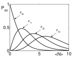
b)

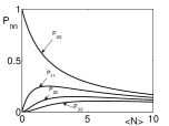
Figure 1: The first four terms $P_{nn}$, $n=0,...,3$ of the joint photon distribution of the state $|x\rangle$ as a function of average photon number $\langle N\rangle$. (a): TMC, (b): TWB.

The states in Eq. (1) are pure states, and therefore we can evaluate their entanglement by the Von Neumann entropy $S_{vn}(x)$ of the reduced density matrix of each subsystem. For the TSS case we simply have:

$$S_{vn}=-P_{00}\log_{2}P_{00}-(1-P_{00})\log_{2}(1-P_{00})$$ (7)

and of course the maximum value of 1 is obtained for $P_{00}=P_{11}=\frac{1}{2}$. The corresponding state $|\Phi_{+}\rangle=\frac{|00\rangle+|11\rangle}{\sqrt{2}}$ is a Bell-like maximally entangled state. For TWB states the Von Neumann Entropy can be written as:

$$S_{vn}(x)=-\log_{2}(1-|x|^{2})-\frac{2|x|^{2}}{1-|x|^{2}}\log_{2}|x|$$ (8)

whereas for TMC states we use the general expression:

$$S_{vn}(x) = -\log_{2}P_{00}(x)-\,$$ (9)

$$- P_{00}(x)\sum_{i=1}^{\infty}|f_{i}(x)|^{2}\log_{2}|f_{i}(x)|^{2}$$

It is clear that the Von Neumann entropy diverges in the limit $|x|\rightarrow 1$ (for TWB) and in the limit $|x|\rightarrow\infty$ (for TMC) because the probability $P_{00}(x)$ vanishes. The VN entropy at fixed energy (average number of photons of the two modes) is maximized by the TWB expression (8). For this reason TWB states are also referred to as maximal entangled states of bipartite CV systems.

We consider the interaction of each radiation mode with a two level atom flying through the cavity. If the interaction time is much shorter than the lifetime of the cavity mode and the atomic decay rates, we can neglect dissipation in system dynamics. On the other hand, we consider the general case of atoms with different interaction times and coupling constants, prepared in superposition states, and off-resonance interaction between each atom and the relative cavity mode. All these features can be quite important in practical implementations such as in cavity QED systems with Rydberg atoms and high-Q microwave cavities Haroche , as noticed in Paternostro2 2004 . In the interaction picture, the interaction Hamiltonian $H_{i}$ is given by:

$$H_{i} = -\hbar\Delta_{A}a^{\dagger}a-\hbar\Delta_{B}b^{\dagger}b+\,$$

$$+ \hbar g_{A}[a^{\dagger}S^{12}_{A,-}+aS^{12}_{A,+}]+\hbar g_{B}[b^{\dagger}S^{12}_{B,-}+bS^{12}_{B,+}]\,$$

where $S^{12}_{A,\pm}$ and $S^{12}_{B,\pm}$ are the lowering and raising atomic operators of the two atoms and $\Delta_{A}$, $\Delta_{B}$ denote the detunings between each mode frequency and the corresponding atomic transition frequency. The initial state of the whole system

$$|\psi(0)\rangle=|x\rangle\otimes|\psi(0)\rangle_{A}\otimes|\psi(0)\rangle_{B}$$

evolves by means of the unitary operator $U(\tau)=\exp[-\frac{i}{\hbar}H_{i}\tau]$ that can be factorized as the product of two off-resonance Jaynes-Cummings evolution operators $U_{A}(\tau)$ and $U_{B}(\tau)$ ORSZAG related to each atom-mode subsystem. For the initial state of both atoms we considered a general superposition of their excited ($|2\rangle$) and ground ($|1\rangle$) states:

$$|\psi(0)\rangle_{A} = A_{2}|2\rangle_{A}+A_{1}|1\rangle_{A}\,$$

$$|\psi(0)\rangle_{B} = B_{2}|2\rangle_{B}+B_{1}|1\rangle_{B}$$ (11)

where $|A_{2}|^{2}+|A_{1}|^{2}=1$ and $|B_{2}|^{2}+|B_{1}|^{2}=1$. This includes the most natural and widely investigated choice of both atoms in the ground states, but will also allow us to investigate the effect of different interaction times.
Due to the linearity of evolution operator $U(\tau)$ and its factorized form, the whole system state $|\psi(\tau)\rangle$ at a time $\tau$ can be written as

$$|\psi(\tau)\rangle=\,$$

$$=c_{0}(x)\sum_{n=0}^{\infty}f_{n}(x)U_{A}(\tau)|\psi^{n}(0)\rangle_{A}\otimes U_{B}(\tau)|\psi^{n}(0)\rangle_{B}\,$$

where $|\psi^{n}(0)\rangle_{A,B}=|\psi(0)\rangle_{A,B}\otimes|n\rangle_{A,B}$. In each of two atom-field subspaces A and B we expand the wave-function on the basis $\{|2\rangle|k\rangle,|1\rangle|k+1\rangle\}^{\infty}_{k=0}\cup\{|0\rangle|1\rangle\}$. The coefficients $c_{A,1,k}(0)=_{A}\langle 2|_{A}\langle k||\psi^{n}(0)\rangle_{A}$ and $c_{B,1,k}(0)=_{B}\langle 2|_{B}\langle k||\psi^{n}(0)\rangle_{B}$ of the initial states are:

$$\begin{array}[]{cc}c_{A,1,0}(0)=A_{1}\delta_{n,0}&c_{B,1,0}(0)=B_{1}\delta_{n,0}\\ c_{A,2,k}(0)=A_{2}\delta_{k,n}&c_{B,2,k}(0)=B_{2}\delta_{k,n}\\ c_{A,1,k+1}(0)=A_{1}\delta_{k+1,n}&c_{B,1,k+1}(0)=B_{1}\delta_{k+1,n}\\ \end{array}$$ (13)

The Jaynes-Cummings interaction couples only the coefficients of each variety $K$ whereas $c_{A,1,0}(0)$, $c_{B,1,0}(0)$ do not evolve. Therefore, for each variety in the subspaces A and B the evolved coefficients can be obtained by applying the off-resonance Jaynes-Cummings $2\times 2$ matrix $U_{jk}$ so that:

$$c_{2,k}(\tau) = U_{11}(k,\tau)c_{2,k}(0)+U_{12}(k,\tau)c_{1,k+1}(0)\,$$

$$c_{1,k+1}(\tau) = U_{21}(k,\tau)c_{2,k}(0)+U_{22}(k,\tau)c_{1,k+1}(0)\,$$

where

$$U_{11}(k,\tau) = \cos(\frac{R_{k}\tau}{2})-i\frac{\Delta}{R_{k}}\sin(\frac{R_{k}\tau}{2})\,$$

$$U_{12}(k,\tau) = -\frac{2ig\sqrt{k+1}}{R_{k}}\sin(\frac{R_{k}\tau}{2})=U_{21}(k,\tau),$$

$$U_{22}(k,\tau) = \cos(\frac{R_{k}\tau}{2})+i\frac{\Delta}{R_{k}}\sin(\frac{R_{k}\tau}{2})\,$$

where the generalized Rabi frequencies are $R_{k}=\sqrt{4g^{2}(k+1)+\Delta^{2}}$. To derive the evolved atomic density operator $\rho_{a}^{1,2}$ we first consider the statistical operator of the whole system $\rho(\tau)=|\psi(\tau)\rangle\langle|\psi(\tau)|$ and then we trace out the field variables. The explicit expressions of the density matrix elements in the standard basis $\{|2\rangle_{A}|2\rangle_{B},|2\rangle_{A}|1\rangle_{B},|1\rangle_{A}|2\rangle_{B},|1\rangle_{A}|1\rangle_{B}\}$ are reported in Appendix A.

III Entanglement transfer at resonance

As a first example we consider exact resonance for both atom-field interactions, equal coupling constant $g$ and the same interaction time $\tau$. For the initial atomic states we will discuss the following three cases: both atoms in the ground state ($|1\rangle_{A}|1\rangle_{B}$), both atoms in the excited state ($|2\rangle_{A}|2\rangle_{B}$), and one atom in the excited state and the other one in the ground state ($|1\rangle_{A}|2\rangle_{B}$). In all these cases the atomic density matrix after the interaction $\rho_{a}^{1,2}$ has the following form:

$$\rho_{a}^{1,2}=\left(\begin{array}[]{cccc}\rho_{11}&0&0&\rho_{14}\\ 0&\rho_{22}&0&0\\ 0&0&\rho_{33}&0\\ \rho_{14}^{*}&0&0&\rho_{44}\\ \end{array}\right)$$ (15)

The presence of the qubit entanglement can be revealed by the Peres-Horodecki criterion peres based on the existence of negative eigenvalues of the partial transpose of Eq. (15). From the expressions of the eigenvalues

$$\lambda_{1}^{PT}=\rho_{44}\hskip 28.45274pt\lambda_{2}^{PT}=\rho_{11}\hskip 28.45274pt\,$$

$$\lambda_{3,4}^{PT}=\frac{\rho_{22}+\rho_{33}\pm\sqrt{(\rho_{22}-\rho_{33})^{2}+4|\rho_{14}|^{2}}}{2}$$ (16)

we see that only $\lambda_{4}^{PT}$ can assume negative values. In the case of TSS the expression of $\lambda_{4}^{PT}$ can allow us to derive in a simple way analytical results for the conditions of maximum entanglement transfer as function of dimensionless interaction time $g\tau$, as well as to better understand the results in the case of TWB and TMC states. In order to quantify the amount of the entanglement and, in turn, to assess the entanglement transfer we choose to adopt the entanglement of formation $\epsilon_{F}$ Bennet . We rewrite the atomic density matrix in the magic basis Magic $\rho_{a}^{MB}$ and we evaluate the eigenvalues of the non-hermitian matrix $R=\rho_{a}^{MB}(\rho_{a}^{MB})^{*}$:

$$\lambda_{1,2}^{R}=\rho_{22}\rho_{33}\hskip 28.45274pt\lambda_{3,4}^{R}=(\sqrt{\rho_{11}\rho_{44}}\pm|\rho_{14}|)^{2}$$ (17)

In this way we calculate the concurrence Wooters $C=max\{0,\Lambda_{1}-\Lambda_{2}-\Lambda_{3}-\Lambda_{4}\}$, where $\Lambda_{i}=\sqrt{\lambda_{i}^{R}}$ are the square roots of the eigenvalues $\lambda_{i}^{R}$ selected in the decreasing order, and then evaluate the entanglement of formation:

$$\epsilon_{F} = -\frac{1-\sqrt{1-C^{2}}}{2}\log_{2}\frac{1-\sqrt{1-C^{2}}}{2}\,$$ (18)

$$- \frac{1+\sqrt{1-C^{2}}}{2}\log_{2}\frac{1+\sqrt{1-C^{2}}}{2}$$

In the case of both qubits initially in the ground state $|1\rangle_{A}|1\rangle_{B}$ the expression of $\lambda_{4}^{PT}$ simply reduces to $\rho_{22}-|\rho_{14}|$, because $\rho_{22}=\rho_{33}$, and it is possible to derive the following simple formula:

$$\lambda_{4}^{PT}(P_{00},g\tau)=\sin^{2}(g\tau)\times\,$$

$$\times[(1-P_{00})\cos^{2}(g\tau)-\sqrt{(1-P_{00})P_{00}}]$$ (19)

We note that only the vacuum Rabi frequency is involved, a fact that greatly simplifies the analysis of atom-field interaction compared to all the other atomic configurations. Let us first consider the Bell-like state ($P_{00}=\frac{1}{2}$) and look for the $g\tau$ values maximizing the entanglement of the two atoms. The solution of equation $\lambda_{4}^{PT}(\frac{1}{2},g\tau)=-\frac{1}{2}$ is given by $g\tau=\frac{\pi}{2}(2k+1)$ with $k=0,1,2,...$. The above condition is relevant also to explain the entanglement transfer for TWB and TMC states, as discussed below. To evaluate the entanglement transfer also for not maximally entangled TSS states in Eq. (2), we calculate the entanglement of formation as a function of both the dimensionless interaction time $g\tau$ and the probability $P_{00}$. As it is apparent from Fig. 2a there are large and well defined regions where $\epsilon_{F}>0$. In particular, the absolute maxima ($\epsilon_{F}=1$) occur exactly at $P_{00}=0.5$ and for $g\tau$ values in agreement with the above series. In addition, if we consider the sections at these $g\tau$ values, we obtain exact coincidence with the Von Neumann Entropy function $S_{vn}(P_{00})$. Therefore, complete entanglement transfer from the field to the atoms is possible not only for the Bell State, though only for the Bell State we may obtain the transferral of 1 ebit.

a)

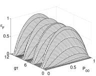
b)

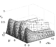
c)

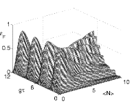
Figure 2: Entanglement of formation $\epsilon_{F}$ of the qubit systems as a function of the dimensionless time $g\tau$ and the CV state parameter $P_{00}$ (a) or the average number of photons $\langle N\rangle$ (b,c) for the case of both atoms initially in the ground state. a) TSS, b) TWB, c) TMC.

In Fig. 2b we consider the entanglement of formation vs $g\tau$ and mean photon number $\langle N\rangle$ in the TWB case. We first note that the regions of maximum entanglement correspond to those of TSS states and the maxima occur at $g\tau$ values close to $\frac{\pi}{2}(2k+1)$, as shown in Table 1.

$g\tau_{max}$	$\langle N\rangle_{max}$	$\epsilon_{F,max}$	$P_{00}$	$P_{11}$
1.56	0.87	0.64	0.69	0.21
4.61	1.82	0.81	0.52	0.25
7.85	1.07	0.68	0.65	0.23
11.03	1.07	0.68	0.65	0.23

Table 1: Maxima of the qubit entanglement of formation $\epsilon_{F}$ for the resonant interaction with TWB and for both qubits initially in the ground state (see Fig. 2b).

We can explain this by considering the TWB photon distribution (see Fig. 1b). We note that the terms $P_{00}$ and $P_{11}$ are always greater or equal than the other terms $P_{nn}$ ($n>1$) and that for $\langle N\rangle<2$ they dominate the photon distribution ($P_{00}+P_{11}\simeq 1$). Therefore, the main contribution to entanglement transfer is obtained from the above two terms as for the TSS state. In order to explain the absolute maximum found in the second peak at $\langle N\rangle=1.82$, we note that in this case $P_{00}$ and $P_{11}$ are closer to the value $0.5$ of a Bell State. In addition, for large $\langle N\rangle$ and $g\tau$ values, there are small regions (not visible in the figure) where entanglement transfer is possible. This is due to the terms $P_{nn}$ ($n>1$) in the photon distribution. In Fig. 2c we show the TMC case and we note that for $\langle N\rangle<4$ there are four well defined peaks where the entanglement is higher than in the TWB case. Also in this case the $g\tau$ values of the maxima (see Table 2) nearly correspond to those of TSS states.

$g\tau_{max}$	$\langle N\rangle_{max}$	$\epsilon_{F,max}$	$P_{00}$	$P_{11}$
1.56	0.89	0.84	0.61	0.34
4.66	1.09	0.90	0.54	0.39
7.85	0.99	0.87	0.57	0.37
11.01	0.99	0.88	0.57	0.37

Table 2: Maxima of the qubit entanglement of formation $\epsilon_{F}$ for the resonant interaction with TMC and for both qubits initially in the ground state (see Fig. 2c).

As in the previous case this can be explained by the TMC photon distribution (see Fig. 1a), where for $\langle N\rangle<4$ the dominant components of the photon distribution are $P_{00}$ and $P_{11}$. The absolute maximum is in the second peak at $\langle N\rangle=1.09$ because $P_{00}$ and $P_{11}$ are even closer to the Bell State than in the other peaks, and this also explains the larger entanglement value $\epsilon_{F}$. For $\langle N\rangle>4$ and large $g\tau$ there are regions with considerable entanglement values, due to the fact that $P_{00}$ and $P_{11}$ are always smaller than the other terms $P_{nn}$ ($n>1$) that dominate the atom-field interaction.We note that the maxima of $\epsilon_{F}$ are higher than in the TWB case.

a)

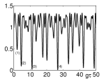
b)

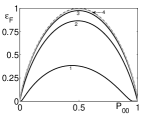
Figure 3: (a): the function $\lambda_{4}^{PT}(\frac{1}{2},g\tau)+\frac{1}{2}$ as in Eq. (III) for the Bell state case with both atoms in the excited state. (b): entanglement of formation $\epsilon_{F}$ vs $P_{00}$ for TSS states compared to Von Neumann entropy (dashed line) for some values of $g\tau$, corresponding to the numbered minima: (1) $2.03$, (2) $4.53$, (3) $11.07$, (4) $26.68$.

A similar analysis can be done in the case of initially excited atoms $|2\rangle_{A}|2\rangle_{B}$. For the TSS states we can again write a simple equation for the eigenvalue of the partial transpose:

$$\lambda_{4}^{PT}(P_{00},g\tau)=(1-P_{00})\sin^{2}(\sqrt{2}g\tau)\cos^{2}(\sqrt{2}g\tau)+\,$$

$$+\sin^{2}(g\tau)[P_{00}\cos^{2}(g\tau)-\sqrt{(1-P_{00})P_{00}}\cos^{2}(\sqrt{2}g\tau)]\,$$

where, with respect to Eq. (III), an additional frequency is present. For the Bell State we can look for $g\tau$ values maximizing the entanglement transfer. In this case the problem can be solved numerically and we found, for example in the range $g\tau=0-50$, that only for $g\tau=26.68\simeq\frac{17\pi}{2}$ we can solve the equation $\lambda_{4}^{PT}(\frac{1}{2},g\tau)=-\frac{1}{2}$ with a good approximation as shown in Fig. 3a. In Fig. 3b we consider also non maximally entangled TSS states, showing the entanglement of formation $\epsilon_{F}$ vs the probability $P_{00}$ for $g\tau$ values corresponding to numbered minima in Fig. 3a. We see that only for $g\tau=26.68$ a Bell State can transfer 1 ebit of entanglement, but the entanglement transfer is complete also for all the other $P_{00}$ values. A nearly complete transfer can be obtained also for $g\tau=11.07$ but in the other cases the entanglement transfer is only partial even for the Bell State. We note that in Zou 2006 it is shown that for $g\tau=11.07$ one finds maximum entanglement transfer for both atomic states $|1\rangle_{A}|1\rangle_{B}$, $|2\rangle_{A}|2\rangle_{B}$ but starting with a different Bell-like field state $|\Psi_{-}\rangle=\frac{|10\rangle-|01\rangle}{\sqrt{2}}$.

In the TWB case we find large entanglement transfer for $g\tau$ values very close to the ones of minima (2-4) for the TSS states in Fig. 3a. Some $g\tau$ values corresponding to maxima of $\epsilon_{F}$ in the case of both atoms in the ground state are missing, and the best value of $\epsilon_{F}$ in the considered range is at $g\tau=26.65$. Also for the TMC states for small $\langle N\rangle$ we have large entanglement transfer corresponding to the above $g\tau$ values, but in addition for $\langle N\rangle>4$ and large $g\tau$ values there are regions with considerable entanglement.
Finally, in the case of one atom in the excited state and the other one in the ground state ($|1\rangle_{A}|2\rangle_{B}$) it is not possible to write for TSS states a simple equation as Eq. (III) because in the atomic density matrix Eq. (15) $\rho_{22}\neq\rho_{33}$ unlike in the previous cases. However, there are again only two frequencies involved as in the TSS case and we can do a similar analysis as for both atoms in the excited state. Here we only mention that for dimensionless interaction times corresponding to common maxima for the different atomic states, the maxima of $\epsilon_{F}$ are rather lower than in the cases ($|1\rangle_{A}|1\rangle_{B}$) and ($|2\rangle_{A}|2\rangle_{B}$), and more in general the transfer of entanglement is sensibly reduced as a function of $\langle N\rangle$.

IV The detuning effect

¿From the practical point of view it is important to evaluate the effects of the off-resonant interaction between the atoms and their respective cavity fields, which can be actually prepared in non degenerate optical parametric processes. We assume equal interaction times for both atoms and we consider first the case of resonant interaction for the atom A and off resonant interaction for atom B. As a first example we consider the TMC case, both atoms in the ground state and the value $g\tau=4.66$, corresponding to the maximum entanglement transfer. In Fig. 4a we see that up to detuning values on the order of the inverse interaction time the entanglement is preserved by the off-resonant interaction of atom B.

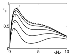
a) b)

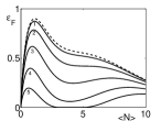
Figure 4: The off resonance interaction effect in the TMC case, both atoms in the ground state and $g\tau=4.66$. a) $\Delta_{A}\tau=0$, and $\Delta_{B}\tau=0$ (dashed line), 1, 2, 3, 4, 5. b) $\Delta_{A}\tau=\Delta_{B}\tau=0$ (dashed line), 1, 2, 3, 4, 5.

In Fig. 4b we show the more general case of off-resonance for both atoms, taking equal detuning values for simplicity. The effect is greater than in the previous case but it is negligible again up to $\Delta_{B}\tau=1$ .
Fig. 5 shows the analogous behaviour for the TWB states for $g\tau=4.61$. We see that near the peak of entanglement the TMC states seem more robust to off resonance interaction than the TWB states.

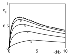
a) b)

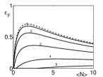
Figure 5: The off resonance interaction effect in the TWB case, both atoms in the ground state and $g\tau=4.61$. a) $\Delta_{A}\tau=0$, and $\Delta_{B}\tau=0$ (dashed line), 1, 2, 3, 4, 5. b) $\Delta_{A}\tau=\Delta_{B}\tau=0$ (dashed line), 1, 2, 3, 4, 5.

V The effect of different interaction times

In the previous analysis we considered equal coupling constant and interaction time for both atoms. However, experimentally we may realize conditions such that the parameter $g\tau$ is different for the two interactions due to the limitations in the control of both atomic velocities and injection times or in the values of the coupling constants Paternostro2 2004 .
We first consider the effect of different interaction times at exact resonance and simultaneous injection of both atoms prepared in the ground state. In Fig. 6a,b we show the TMC case for $g\tau_{A}=4.66$ and $g\tau_{A}=11.01$, corresponding to two maxima of entanglement as discussed in the previous section, and we investigate the effect of different dimensionless interaction times for the atom B such that $g\tau_{B}\leq g\tau_{A}$. We see that increasing the difference $g\tau_{A}-g\tau_{B}$ the entanglement decreases.

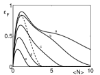
a) b)

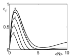
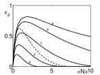
c) d)

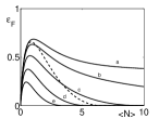
Figure 6: The effect of different interaction times for $\Delta_{A}=\Delta_{B}=0$, and both atoms injected simultaneously in the ground state. In a) the TMC case for $g\tau_{A}=4.66$ and $g\tau_{B}$ values: a) 4.66, b) 4.4, c) 4.2, d) 4.0, e) 3.8, and 1.56 (dashed line). In b) the TMC case for $g\tau_{A}=11.01$ and $g\tau_{B}$ values: a) 11.01, b) 10.8, c) 10.6, d) 10.4, e) 10.2 and 7.85 (dashed line). In c) the TWB case for $g\tau_{A}=4.61$ and $g\tau_{B}$ values: a) 4.61, b) 4.4, c) 4.2, d) 4.0, e) 3.8, and 1.56 (dashed line). In d) the TWB case for $g\tau_{A}=11.03$ and $g\tau_{B}$ values: a) 11.03, b) 10.8, c) 10.6, d) 10.4, e) 10.2 and 7.85 (dashed line).

However for $\langle N\rangle<4$, if $g\tau_{B}$ has a value close to the one corresponding to a maximum, as for $g\tau_{A}=1.56$ in Fig. 6a and $g\tau_{A}=7.85$ in Fig. 6b, i.e. if $g\tau_{A}-g\tau_{B}\cong\pi$, the entanglement reaches again large values. The effect is more important for $g\tau_{A}=11.01$ where the entanglement transfer is the same as for equal interaction times. In Fig. 6c,d we show an analogous effect for the TWB case. We finally consider the possibility that atom B enters the cavity just before atom A. We assume that when atom A enters its cavity the two mode field can be still described by Eq. (1). Due to the interaction with its cavity field the atom B will be in a superposition state $B_{1}|1\rangle_{B}+B_{2}|2\rangle_{B}$. In this case the atomic density matrix $\rho_{a}^{12}$ has only two null elements, $\rho_{23}=\rho_{32}^{*}$, hence we evaluate the eigenvalues of the non-hermitian matrix numerically. We calculate the amount of entanglement transferred to the atoms after the time $\tau$ of their simultaneous presence into the respective cavities in the case of exact resonance, equal coupling constant and velocity, assuming atom A prepared in the ground state. In Fig. 7a we show the TMC case for $g\tau=4.66$ and different values of $|B_{1}|^{2}$ ranging from 0 (that is for $|1\rangle_{A}|2\rangle_{B}$) to 1 (that is $|1\rangle_{A}|1\rangle_{B}$). We note that the behaviour of $\epsilon_{F}$ gradually changes from one limit case to the other one for $\langle N\rangle<4$, when the photon distribution approaches that of a TSS state. For larger values of $\langle N\rangle$ we see the occurrence of a second peak in the case $|1\rangle_{A}|2\rangle_{B}$. In Fig. 7b we show the TWB case for $g\tau=4.61$ and we note that the gradual change described above occurs for nearly all values of the mean photon number $\langle N\rangle$.

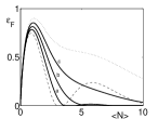
a) b)

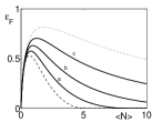
Figure 7: The entanglement of formation $\epsilon_{F}$ vs $\langle N\rangle$ for a time $g\tau$ of simultaneous presence of both atoms after the delayed injection of atom A. Atom A is prepared in the ground state and atom B in superposition states such that $|B_{1}|^{2}=0$ (dashed line), 0.25 (a), 0.50 (b), 0.75 (c), 1 (dotted line). a) the TMC case with $g\tau=4.66$. b) the TWB case with $g\tau=4.61$.

VI Conclusions

In this paper we have addressed the transfer of entanglement from a bipartite state of a continuous-variable system to a pair of localized qubits. We have assumed that each CV mode couples to one qubit via the Jaynes-Cummings interaction and have taken into account the degrading effects of detuning and of different interaction times for the two subsystems. The transfer of entanglement has been assessed by tracing out the field degrees of freedom after the interaction, and then evaluating the entanglement of formation of the reduced atomic density matrix.
We found that CV states initially prepared in a two-state superposition are the most efficient in transferring entanglement to qubits with Bell-like states able to transfer a full ebit of entanglement. We have then considered multiphoton preparation as TWB and TMC states and found that there are large and well defined regions of interaction parameters where the transfer of entanglement is effective. At fixed energy (average number of photons) TMC states are more effective in transferring entanglement than TWB states. We have also found that the entanglement transfer is robust against the fluctuations of interaction times and is not dramatically affected by detuning. This kind of robustness is enhanced for the transfer of entanglement from non Gaussian states as TMC states.
Overall, we conclude that the scheme analyzed in this paper is a reliable and robust mechanism for the engineering of the entanglement between two atomic qubits and that bipartite non Gaussian states are promising resources in order to optimize this protocol. Finally, we mention that our analysis may also be employed to assess the entanglement transfer from radiation to superconducting qubits.

Appendix A ATOMIC DENSITY MATRIX ELEMENTS

The elements of the $4\times 4$ atomic density matrix $\rho_{a}^{12}$ in the standard basis $\{|2\rangle_{A}|2\rangle_{B},|2\rangle_{A}|1\rangle_{B},|1\rangle_{A}|2\rangle_{B},|1\rangle_{A}|1\rangle_{B}\}$ are listed below.

$$\rho_{11}(x)=|c_{0}(x)|^{2}\{|A_{2}|^{2}|B_{2}|^{2}\sum_{j=0}^{\infty}|f_{j}(x)|^{2}|U_{A11}(j,\tau)|^{2}|U_{B11}(j,\tau)|^{2}+\,$$

$$+A_{1}^{*}A_{2}B_{1}^{*}B_{2}\sum_{j=0}^{\infty}f_{j}(x)f_{j+1}^{*}(x)U_{A11}(j,\tau)U_{B11}(j,\tau)U_{A12}^{*}(j,\tau)U_{B12}^{*}(j,\tau)+\,$$

$$+|A_{2}|^{2}|B_{1}|^{2}\sum_{j=0}^{\infty}|f_{j+1}(x)|^{2}|U_{A11}(j+1,\tau)|^{2}|U_{B12}(j,\tau)|^{2}+|A_{1}|^{2}|B_{2}|^{2}\sum_{j=0}^{\infty}|f_{j+1}(x)|^{2}|U_{A12}(j,\tau)|^{2}|U_{B11}(j+1,\tau)|^{2}+\,$$

$$+|A_{1}|^{2}|B_{1}|^{2}\sum_{j=0}^{\infty}|f_{j+1}(x)|^{2}|U_{A12}(j,\tau)|^{2}|U_{B12}(j,\tau)|^{2}+\,$$

$$+A_{1}A_{2}^{*}B_{1}B_{2}^{*}\sum_{j=0}^{\infty}f_{j+1}(x)f_{j}^{*}(x)U_{A12}(j,\tau)U_{B12}(j,\tau)U_{A11}^{*}(j,\tau)U_{B11}^{*}(j,\ tau)\}$$ (21)

$$\rho_{22}(x)=|c_{0}(x)|^{2}\{|A_{2}|^{2}|B_{2}|^{2}\sum_{j=1}^{\infty}|f_{j-1}(x)|^{2}|U_{A11}(j-1,\tau)|^{2}|U_{B21}(j-1,\tau)|^{2}+\,$$

$$+A_{1}^{*}A_{2}B_{1}^{*}B_{2}\sum_{j=1}^{\infty}f_{j-1}(x)f_{j}^{*}(x)U_{A11}(j-1,\tau)U_{B21}(j-1,\tau)U_{A12}^{*}(j-1,\tau)U_{B22}^{*}(j-1,\tau)+\,$$

$$+|A_{2}|^{2}|B_{1}|^{2}[\sum_{j=1}^{\infty}|f_{j}(x)|^{2}|U_{A11}(j,\tau)|^{2}|U_{B22}(j-1,\tau)|^{2}+|U_{A11}(0,\tau)|^{2}]+\,$$

$$+|A_{1}|^{2}|B_{2}|^{2}\sum_{j=1}^{\infty}|f_{j}(x)|^{2}|U_{A12}(j-1,\tau)|^{2}|U_{B21}(j,\tau)|^{2}+|A_{1}|^{2}|B_{1}|^{2}\sum_{j=1}^{\infty}|f_{j}(x)|^{2}|U_{A12}(j-1,\tau)|^{2}|U_{B22}(j-1,\tau)|^{2}+\,$$

$$+A_{1}A_{2}^{*}B_{1}B_{2}^{*}\sum_{j=1}^{\infty}f_{j}(x)f_{j-1}^{*}(x)U_{A12}(j-1,\tau)U_{B22}(j-1,\tau)U_{A11}^{*}(j-1,\tau)U_{B21}^{*}(j-1,\tau)\}$$ (22)

$$\rho_{33}(x)=|c_{0}(x)|^{2}\{|A_{2}|^{2}|B_{2}|^{2}\sum_{j=0}^{\infty}|f_{j}(x)|^{2}|U_{A21}(j,\tau)|^{2}|U_{B11}(j,\tau)|^{2}+\,$$

$$+A_{1}^{*}A_{2}B_{1}^{*}B_{2}\sum_{j=0}^{\infty}f_{j}(x)f_{j+1}^{*}(x)U_{A21}(j,\tau)U_{B11}(j,\tau)U_{A22}^{*}(j,\tau)U_{B12}^{*}(j,\tau)+\,$$

$$+|A_{1}|^{2}|B_{2}|^{2}[\sum_{j=1}^{\infty}|f_{j}(x)|^{2}|U_{A22}(j-1,\tau)|^{2}|U_{B11}(j,\tau)|^{2}+|U_{B11}(0,\tau)|^{2}]+\,$$

$$+|A_{2}|^{2}|B_{1}|^{2}\sum_{j=0}^{\infty}|f_{j+1}(x)|^{2}|U_{A21}(j+1,\tau)|^{2}|U_{B12}(j,\tau)|^{2}+|A_{1}|^{2}|B_{1}|^{2}\sum_{j=0}^{\infty}|f_{j+1}(x)|^{2}|U_{A22}(j,\tau)|^{2}|U_{B12}(j,\tau)|^{2}+\,$$

$$+A_{1}A_{2}^{*}B_{1}B_{2}^{*}\sum_{j=0}^{\infty}f_{j+1}(x)f_{j}^{*}(x)U_{A22}(j,\tau)U_{B12}(j,\tau)U_{A21}^{*}(j,\tau)U_{B11}^{*}(j,\tau)\}$$ (23)

$$\rho_{44}(x)=|c_{0}(x)|^{2}\{|A_{2}|^{2}|B_{2}|^{2}\sum_{j=1}^{\infty}|f_{j-1}(x)|^{2}|U_{A21}(j-1,\tau)|^{2}|U_{B21}(j-1,\tau)|^{2}+\,$$

$$+A_{1}^{*}A_{2}B_{1}^{*}B_{2}\sum_{j=1}^{\infty}f_{j-1}(x)f_{j}^{*}(x)U_{A21}(j-1,\tau)U_{B21}(j-1,\tau)U_{A22}^{*}(j-1,\tau)U_{B22}^{*}(j-1,\tau)+\,$$

$$+|A_{2}|^{2}|B_{1}|^{2}[\sum_{j=1}^{\infty}|f_{j}(x)|^{2}|U_{A21}(j,\tau)|^{2}|U_{B22}(j-1,\tau)|^{2}+|U_{A21}(0,\tau)|^{2}]+\,$$

$$+|A_{1}|^{2}|B_{2}|^{2}[\sum_{j=1}^{\infty}|f_{j}(x)|^{2}|U_{A22}(j-1,\tau)|^{2}|U_{B21}(j,\tau)|^{2}+|U_{B21}(0,\tau)|^{2}]+\,$$

$$+|A_{1}|^{2}|B_{1}|^{2}[\sum_{j=1}^{\infty}|f_{j}(x)|^{2}|U_{A22}(j-1,\tau)|^{2}+|U_{B22}(j-1,\tau)|^{2}+1]+\,$$ (24)

$$+A_{1}A_{2}^{*}B_{1}B_{2}^{*}\sum_{j=1}^{\infty}f_{j}(x)f_{j-1}^{*}(x)U_{A22}(j-1,\tau)U_{B22}(j-1,\tau)U_{A21}^{*}(j-1,\tau)U_{B21}^{*}(j-1,\tau)\}$$

$$\rho_{12}(x)=|c_{0}(x)|^{2}\{|A_{2}|^{2}B_{1}^{*}B_{2}[\sum_{j=1}^{\infty}|f_{j}(x)|^{2}|U_{A11}(j,\tau)|^{2}U_{B11}(j,\tau)U_{B22}^{*}(j-1,\tau)+|U_{A11}(0,\tau)|^{2}U_{B11}(0,\tau)]+\,$$

$$+|A_{1}|^{2}B_{2}B_{1}^{*}\sum_{j=1}^{\infty}|f_{j}(x)|^{2}U_{A12}(j-1,\tau)|^{2}|U_{B11}(j,\tau)U_{B22}^{*}(j-1,\tau)+\,$$

$$+A_{1}A_{2}^{*}|B_{2}|^{2}\sum_{j=1}^{\infty}f_{j}(x)f_{j-1}^{*}(x)U_{A12}(j-1,\tau)U_{B11}(j,\tau)U_{A11}^{*}(j-1,\tau)U_{B21}^{*}(j-1,\tau)+\,$$

$$+A_{1}A_{2}^{*}|B_{1}|^{2}[\sum_{j=1}^{\infty}f_{j+1}(x)f_{j}^{*}(x)U_{A12}(j,\tau)U_{B12}(j,\tau)U_{A11}^{*}(j,\tau)U_{B22}^{*}(j-1,\tau)+f_{1}(x)U_{A12}(0,\tau)U_{B12}(0,\tau)U_{A11}^{*}(0,\tau)]\}\,$$

$$\rho_{13}(x)=|c_{0}(x)|^{2}\{|A_{2}|^{2}B_{1}B_{2}^{*}\sum_{j=0}^{\infty}f_{j+1}(x)f_{j}^{*}(x)U_{A11}(j+1,\tau)U_{B12}(j,\tau)U_{A21}^{*}(j,\tau)U_{B11}^{*}(j,\tau)+\,$$

$$+|A_{1}|^{2}B_{1}B_{2}^{*}[\sum_{j=1}^{\infty}f_{j+1}(x)f_{j}^{*}(x)U_{A12}(j,\tau)U_{B12}(j,\tau)U_{A22}^{*}(j-1,\tau)U_{B11}^{*}(j,\tau)+f_{1}(x)U_{A12}^{(}0,\tau)U_{B12}(0,\tau)U_{B11}^{*}(0,\tau)]+\,$$

$$+A_{1}^{*}A_{2}|B_{2}|^{2}[\sum_{j=1}^{\infty}|f_{j}(x)|^{2}U_{A11}(j,\tau)|U_{B11}(j,\tau)|^{2}U_{A22}^{*}(j-1,\tau)+U_{A11}(0,\tau)|U_{B11}(0,\tau)|^{2}]+\,$$

$$+A_{1}^{*}A_{2}|B_{1}|^{2}\sum_{j=0}^{\infty}|f_{j+1}(x)|^{2}U_{A11}(j+1,\tau)|U_{B12}(j,\tau)|^{2}U_{A22}^{*}(j,\tau)\}$$ (26)

$$\rho_{14}(x)=|c_{0}(x)|^{2}\{|A_{2}|^{2}|B_{2}|^{2}\sum_{j=1}^{\infty}f_{j}(x)f_{j-1}^{*}(x)U_{A11}(j,\tau)U_{B11}(j,\tau)U_{A21}^{*}(j-1,\tau)U_{B21}^{*}(j-1,\tau)+\,$$

$$+A_{1}^{*}A_{2}B_{1}^{*}B_{2}[\sum_{j=1}^{\infty}|f_{j}(x)|^{2}U_{A11}(j,\tau)U_{B11}(j,\tau)U_{A22}^{*}(j-1,\tau)U_{B22}^{*}(j-1,\tau)+U_{A11}(0,\tau)U_{B11}(0,\tau)]+\,$$

$$+|A_{2}|^{2}|B_{1}|^{2}[\sum_{j=1}^{\infty}f_{j}(x)f_{j-1}^{*}(x)U_{A11}(j+1,\tau)U_{B12}(j,\tau)U_{A21}^{*}(j,\tau)U_{B22}^{*}(j-1,\tau)+\,$$

$$+f_{1}(x)U_{A11}(1,\tau)U_{B12}(0,\tau)U_{A21}^{*}(0,\tau)]+\,$$

$$+|A_{1}|^{2}|B_{2}|^{2}[\sum_{j=1}^{\infty}f_{j+1}(x)f_{j}^{*}(x)U_{A12}(j,\tau)U_{B11}(j+1,\tau)U_{A22}^{*}(j-1,\tau)U_{B21}^{*}(j,\tau)+\,$$

$$+f_{1}(x)U_{A12}(0,\tau)U_{B11}(1,\tau)U_{B12}^{*}(0,\tau)]+\,$$

$$+|A_{1}|^{2}|B_{1}|^{2}[\sum_{j=1}^{\infty}f_{j+1}(x)f_{j}^{*}(x)U_{A12}(j,\tau)U_{B12}(j,\tau)U_{A22}^{*}(j-1,\tau)U_{B22}^{*}(j-1,\tau)+\,$$ (27)

$$+f_{1}(x)U_{A12}(0,\tau)U_{B12}(0,\tau)]+\,$$

$$+A_{1}A_{2}^{*}B_{1}B_{2}^{*}\sum_{j=1}^{\infty}f_{j+1}(x)f_{j-1}^{*}(x)U_{A12}(j,\tau)U_{B12}(j,\tau)U_{A21}^{*}(j-1,\tau)U_{B21}^{*}(j-1,\tau)\}$$

$$\rho_{23}(x)=|c_{0}(x)|^{2}A_{1}^{*}A_{2}B_{1}B_{2}^{*}[\sum_{j=0}^{\infty}|f_{j}(x)|^{2}U_{A11}(j,\tau)U_{B22}(j-1,\tau)U_{A22}^{*}(j-1,\tau)U_{B11}^{*}(j,\tau)+U_{A11}(0,\tau)U_{B11}^{*}(0,\tau)]\,$$

$$\rho_{24}(x)=|c_{0}(x)|^{2}\{|A_{2}|^{2}B_{1}B_{2}^{*}\sum_{j=1}^{\infty}f_{j}(x)f_{j-1}^{*}(x)U_{A11}(j,\tau)U_{B22}(j-1,\tau)U_{A21}^{*}(j-1,\tau)U_{B21}^{*}(j-1,\tau)+\,$$

$$+|A_{1}|^{2}B_{1}B_{2}^{*}[\sum_{j=1}^{\infty}f_{j+1}(x)f_{j}^{*}(x)U_{A12}(j,\tau)U_{B22}(j,\tau)U_{A22}^{*}(j-1,\tau)U_{B21}^{*}(j,\tau)+\,$$

$$+f_{1}(x)U_{A12}^{(}0,\tau)U_{B22}(0,\tau)U_{B21}^{*}(0,\tau)]+\,$$

$$+A_{1}^{*}A_{2}|B_{2}|^{2}[\sum_{j=1}^{\infty}|f_{j}(x)|^{2}U_{A11}(j,\tau)|U_{B21}(j,\tau)|^{2}U_{A22}^{*}(j-1,\tau)+U_{A11}(0,\tau)|U_{B21}(0,\tau)|^{2}]+\,$$

$$+A_{1}^{*}A_{2}|B_{1}|^{2}[\sum_{j=1}^{\infty}|f_{j}(x)|^{2}U_{A11}(j,\tau)|U_{B22}(j-1,\tau)|^{2}U_{A12}^{*}(j-1,\tau)+U_{A11}(0,\tau)]\}$$ (29)

$$\rho_{34}(x)=|c_{0}(x)|^{2}\{|A_{2}|^{2}B_{1}^{*}B_{2}[\sum_{j=1}^{\infty}|f_{j}(x)|^{2}|U_{A21}(j,\tau)|^{2}U_{B11}(j,\tau)U_{B22}^{*}(j-1,\tau)+|U_{A21}(0,\tau)|^{2}U_{B11}(0,\tau)\,$$

$$+ |A_{1}|^{2}B_{1}^{*}B_{2}[\sum_{j=1}^{\infty}|f_{j}(x)|^{2}U_{A22}(j-1,\tau)U_{B11}(j,\tau)U_{A22}^{*}(j-1,\tau)U_{B22}^{*}(j-1,\tau)+U_{B11}(0,\tau)]\,$$

$$+ A_{1}A_{2}^{*}|B_{2}|^{2}\sum_{j=1}^{\infty}f_{j}(x)f_{j-1}^{*}(x)U_{A22}(j-1,\tau)U_{B11}(j,\tau)U_{A21}^{*}(j-1,\tau)U_{B21}^{*}(j-1,\tau)\,$$

$$+ A_{1}^{*}A_{2}|B_{1}|^{2}[\sum_{j=1}^{\infty}f_{j+1}(x)f_{j}^{*}(x)U_{A22}(j,\tau)U_{B12}(j,\tau)U_{A21}^{*}(j,\tau)U_{B22}^{*}(j-1,\tau)+f_{1}(x)U_{A22}(0,\tau)U_{B12}(0,\tau)U_{A21}^{*}(0,\tau)]\}\,$$

References

- (1) B. Julsgaard, J. Sherson, J.I. Cirac, J. Fiur sek, and E.S. Polzik, Nature 432 482 (2004).
- (2) M. D. Eisaman, A. Andr , F. Massou, M. Fleischhauer, A. S. Zibrov and M. D. Lukin, Nature 438, 837 (2005); T. Chaneli re, D. N. Matsukevich, S. D. Jenkins, S.-Y. Lan, T. A. B. Kennedy and A. Kuzmich, Nature 438, 833 (2005).
- (3) H. J. Briegel, W. Dür, J. I. Cirac, and P. Zoller, Phys. Rev. Lett. 81, 5932 (1998).
- (4) R. Cleve and H. Buhrman, Phys. Rev. A 56, 1201 (1997).
- (5) B. Kraus and J.I. Cirac, Phys. Rev. Lett. 92, 013602 (2004).
- (6) M. Paternostro, W. Son, and M.S. Kim, Phys. Rev. Lett. 92, 197901 (2004).
- (7) M. Paternostro, W. Son, M.S. Kim, G. Falci, and G.M. Palma, Phys. Rev. A. 70, 022320 (2004).
- (8) M. Paternostro, G. Falci, M. Kim, and G.M. Palma, Phys. Rev. B. 69, 214502 (2004).
- (9) A. Ferraro, S. Olivares and M. G. A. Paris, “Gaussian States in Quantum Information ”, Napoli Series on Physics and Astrophysics (Bibliopolis, Napoli, 2005).
- (10) J. Lee, M. S. Kim, and H. Jeong, Phys. Rev A 62, 032305 (2000);J. S. Prauzner-Bechcicki, J. Phys. A 37, L173 (2004); A. Vukics, J. Janszky, and T. Kobayashi, Phys. Rev. A 66, 023809 (2002); W. P. Bowen, N. Treps, B. C. Buchler, R. Schnabel, T.C. Ralph, H.-A. Bachor, T. Symul, and P. K. Lam, Phys. Rev. A 67, 032302 (2003); S. Olivares, M. G. A. Paris, and A. R. Rossi, Phys. Lett. A 319, 32 (2003); A. Serafini, F. Illuminati, M. G. A. Paris, and S. De Siena, Phys. Rev A 69, 022318 (2004).
- (11) J. Hald, J.L. Sorensen, C. Shori, and E.S. Polzik, J. Mod. Opt. 47, 2599 (2000).
- (12) W. Son, M. S. Kim, J. Lee, and D. Ahn, J. Mod. Opt. 49, 1739 (2002).
- (13) B.L. Schumaker, and C.M. Caves, Phys. Rev. A 31 3093 (1985); S.M. Barnett and P.L. Knight, J. Mod. Opt. 34, 841 (1987); K. Watanabe and Y. Yamamoto, Phys. Rev. A 38, 3556 (1988).
- (14) J. Zou, G.L. Jun, S. Bin, L. Jian, and S.L. Qian, Phys. Rev. A 73, 042319 (2006).
- (15) J. Lee, M. Paternostro, M.S. Kim, and S. Bose, Phys. Rev. Lett. 96, 080501 (2006).
- (16) D. McHugh, M. Ziman, and V. Buzek, Phys. Rev. A. 74, 042303 (2006).
- (17) A. Serafini, M. Paternostro, M. S. Kim, and S. Bose, Phys. Rev. A. 73, 022312 (2006).
- (18) G.S. Agarwal, Phys. Rev. Lett. 57, 827 (1986); G.S. Agarwal, J. Opt. Soc. Am. B 5, 1940 (1988).
- (19) S. Zheng and G. C. Guo, Z. Phys. B 103, 311 (1997); S. Zheng, Physica A 260, 439 (1998).
- (20) X. Zou, Y. Dong, and G. Guo, Phys. Rev. A. 74, 015801 (2006).
- (21) M.D. Reid and L. Krippner, Phys. Rev. A. 47, 552 (1993)
- (22) A. Gilchrist and W. J. Munro, J. Opt. B: Quantum Semiclass. Opt. 1, 47 (2000).
- (23) J.M. Raimond, M. Brune, and S. Haroche, Rev. Mod. Phys 73, 265 (2001).
- (24) see e.g. C.C. Gerry and P.L. Knight, ”Introductory quantum optics” (Cambridge University Press, Cambridge, 2005).
- (25) A. Peres, Phys. Rev. Lett. 77, 1413 (1996); M. Horodecki, P. Horodecki, and R. P. Horodecki, Phys.Lett. A 223, 1 (1996).
- (26) C.H. Bennett, D.P. Di Vincenzo, J.A. Smolin, and W.K. Wootters, Phys. Rev. A. 54, 3824 (1996).
- (27) S. Hill and W.K. Wootters, Phys. Rev. Lett. 78, 5022 (1997).
- (28) W.K. Wootters, Phys. Rev. Lett. 80, 2245 (1998).