On the measurement probability of quantum phases

Abstract

We consider the probability by which quantum phase measurements of a given precision can be done successfully. The least upper bound of this probability is derived and the associated optimal state vectors are determined. The probability bound represents an unique and continuous transition between macroscopic and microscopic measurement precisions.

The classical picture for the evolution of a single-mode electromagnetic field is simply determined by an amplitude (specifying the strength of the field) and a phase (specifying the zeros of the field). On the other hand, the concept of electromagnetic phase as an observable quantity is a long-standing problem of quantum optics and it has been the question whether there exists a phase observable that is canonically conjugate to the number observable for a single-mode field. The quantum mechanical description of phase was first considered by London L26 and Dirac D27 . An obvious way of defining an operator for the phase is by polar decomposition of the photon annihilation operator $\hat{a}=e^{i\hat{\phi}}\sqrt{\hat{N}}$. The phase operator $\hat{\phi}$ defined in this way is equivalent to that considered by Dirac D27 , who obtained the commutator $[\hat{\phi},\hat{N}]=i$ by employing the correspondence between commutators and classical Poisson bracket. Formally, this would imply the uncertainty relation

$$\sigma_{\phi}\sigma_{N}\geq\frac{1}{2}$$ (1)

with $\sigma_{\phi}$ and $\sigma_{N}$ are the standard deviations of $\phi$ and $N$. The difficulties of Dirac’s approach were clearly pointed out by Susskind and Glogower SG64 . Firstly, the relation (1) would imply that a well-defined number state would have a phase standard deviation greater than $2\pi$. This is a consequence of the fact that Dirac’s commutator does not take account of the periodic nature of the phase. Furthermore, the exponential operator $e^{i\hat{\phi}}$ derived from this approach is not unitary and thus does not define a Hermitian operator. This is why it is often accepted that a well-behaved Hermitian phase operator does not exist SG64 ; CN68 . Therefore, arguments based on the Heisenberg relation (1) cannot hold in general.

Actually, the standard deviation offers a reasonable measure of the spread of values when the distribution in question is of a simple "single hump" type. In particular it is a very good characteristic for a Gaussian distribution since it measures directly the half-width of this distribution. However, when the distribution is not of a simple type (for example, has more than one hump) the standard deviation loses much of its usefulness as a measure of uncertainty.

The aim of the present contribution is to introduce the probability by which a successful phase measurements of a given precision can be done. The least upper bound of this probability is determined and the corresponding (optimal) state vectors are computed.

In order to specify phase measurements, the probability distribution for the measurement result can be determined using positive operator-valued measures. This approach was first considered by Helstrom H76 , and is also considered in SSW89 ; SS91 . Precisely, let $\cal{H}$ be a complex separable Hilbert space, $(|n\rangle)_{n\geq 0}$ an orthonormal basis, and $N=\sum_{n=0}^{\infty}n|n\rangle\langle n|$ the associated number observable. If the phase density $F_{\phi}$ treats all phases equally, it should be invariant under phase translation, $e^{i\theta N}F_{\phi}e^{-i\theta N}=F_{\phi+\theta}$, generated by the number observable. In this case, the general form of $F_{\phi}$ is

$$F_{\phi}=\frac{1}{2\pi}\,\sum_{n,m=0}^{\infty}c_{nm}\,e^{i(n-m)\phi}\;\;|n\rangle\langle m|$$ (2)

where $(c_{nm})$ is the associated phase matrix. For the integral of the probability to equal 1, we must have

$$\int_{-\pi}^{\pi}F_{\phi}\,d\phi=1.$$ (3)

Applying this to (2) above we find that delta

$$\sum_{n=0}^{\infty}c_{nn}\;|n\rangle\langle n|=1.$$ (4)

This means that the diagonal elements $c_{nn}$ must all be equal to 1. The additional condition of positive definite probabilities, together with the above result means that all of the $c_{nm}$ must have absolute values between 0 and 1. In general, real measurements will give smaller values of $c_{nm}$, and the closer these are to 1 the better the phase measurement is. In LVBP95 it is shown that the additional condition that a number shifter does not alter the phase distribution gives $c_{nm}=1$, corresponding to the canonical measure LVBP95

$$E_{\phi}=\frac{1}{2\pi}\,\sum_{n,m=0}^{\infty}e^{i(n-m)\phi}\;\;|n\rangle\langle m|.$$ (5)

An alternative derivation of this result is by using the maximum likelihood approach SSW89 . Note that (5) may be expressed by $dE_{\phi}=|\phi\rangle\langle\phi|\,d\phi$, where

$$|\phi\rangle=\frac{1}{\sqrt{2\pi}}\sum_{n=0}^{\infty}e^{in\phi}|n\rangle$$ (6)

With reference to (5), we now define the precision $\Delta\alpha\in[0,2\pi)$ of a phase measurement corresponding to the vicinity $A_{\alpha}=[\alpha-\frac{\Delta\alpha}{2},\alpha+\frac{\Delta\alpha}{2})$ of any value $\alpha\in[-\pi,\pi)$. The probability of a phase measurement with $\phi\in A_{\alpha}$, made on a state described by a density operator $\hat{\rho}$, is given by

$$P_{\alpha}(\Delta\alpha)=\mbox{Tr}[\hat{\rho}\,E_{\phi}(A_{\alpha})].$$ (7)

On the other hand, the probability to measure a photon number $n\in B_{k}$ is given by

$$P_{k}(\Delta k)=\mbox{Tr}[\hat{\rho}\,E_{N}(B_{k})]$$ (8)

where

$$E_{N}(B_{k})=\sum_{n\in B_{k}}\,|n\rangle\langle n|$$ (9)

is the value of the spectral measure $E_{N}$ on a set $B_{k}$ of positive integers. In order to introduce the precision $\Delta k\in\mathbb{N}$ by which the photon number is measured, we note that the photon number is bounded from below. Therefore, we define the right-sided vicinity $B_{k}\subset\mathbb{N}$ of $k$ by $B_{k}=\{k,k+1,...,k+\Delta k\}$. In this definition, the integer $k$ is the smallest element of $B_{k}$. Alternative definitions are also possible but typically lead to necessary readjustments in certain cases for $k<\Delta k$. However, it will be seen later that our results are not dependent on the particular subscription. For technical purposes we apply the definition of the minimum integer-subscription. In the case of pure states $\hat{\rho}=|\psi\rangle\langle\psi|$, we obtain the probability

$$P_{k}(\Delta k)=\sum_{n=k}^{k+\Delta k}|\psi_{n}|^{2}$$ (10)

and $\psi_{n}=\langle n|\psi\rangle$ is the number-space amplitude of $\psi$.

Now, we consider the case with an initial photon number preparation of a state $\psi$. A single mode is supposed to emerge in a state according to

$$\psi\to\psi^{\prime}=\frac{E_{N}(B_{k})\psi}{||E_{N}(B_{k})\psi||}.$$ (11)

Afterwards, the number of photons is given with precision $\Delta k$. In this situation the uncertainty principle suggests that the more accurately the number is measured the greater is the perturbation of the phase of the outgoing state. The conditional probability ${\cal P}_{\alpha k}(\Delta\alpha\,|\,\Delta k;\psi)$ to measure phase $\phi\in A_{\alpha}$, on the state transformed by the initial number measurement, is given by

$${\cal P}_{\alpha k}(\Delta\alpha\,|\,\Delta k;\psi)=\frac{||E_{\phi}(A_{\alpha})E_{N}(B_{k})\,\psi||^{2}}{||E_{N}(B_{k})\,\psi||^{2}}$$ (12)

We now ask for the least upper bound $\lambda_{0}$ of the measurement probability (12) and we end up in a variation problem in Hilbert space with three degrees of freedom. For fixed precisions $\Delta k$ and $\Delta\alpha$ we are searching for the supremum of (12) by variation of the parameters $\alpha$, $k$ and the state vector $\psi$ of the photon. Actually this variation problem is translation and rotation invariant in Hilbert space and we can simply chose $k=0$ and $\alpha=0$ without loss of generality. After all, we have to consider the following expression

$$\lambda_{0}=\sup\limits_{\psi\in{\cal H}\setminus\{0\}}{\cal P}_{00}(\Delta\alpha\,|\,\Delta k;\psi)$$ (13)

and by using (5) and (9) we explicitly obtain to following expression

$${\cal P}_{00}(\Delta\alpha\,|\,\Delta k;\psi)=\frac{\int\limits_{-\Delta\alpha/2}^{\Delta\alpha/2}\left|\frac{1}{\sqrt{2\pi}}\sum\limits_{n=0}^{\Delta k}\psi_{n}\,e^{in\phi}\right|^{2}d\phi}{\sum\limits_{n^{\prime}=0}^{\Delta k}|\psi_{n^{\prime}}|^{2}}.$$ (14)

Applying the Cauchy-Bunyakovsky inequality we obtain the following general upper bound

$${\cal P}_{\alpha,k}(\Delta\alpha\,|\,\Delta k;\psi)\leq\frac{\Delta\alpha(\Delta k+1)}{2\pi}$$ (15)

for every $\Delta\alpha\in[-\pi,\pi)$ and integer $\Delta k\geq 0$. In fig. 1, the set of impossible measurement processes is expressed by the grey shaded triangle.

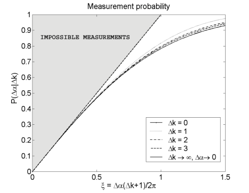
Figure 1: Maximum eigenvalue $\lambda_{0}$ for $\Delta k=0,1,2,3,\infty$ (from left to right). Phase measuring processes with probabilities larger than $\lambda_{0}$ do not exist.

In order to reach even tighter bounds we explicitly computed the integral in (14) and applied certain trigonometric identities to obtain the following expression

$${\cal P}_{00}(\Delta\alpha\,|\,\Delta k;\psi)=\sum\limits_{n,m=0}^{\infty}G_{nm}\,\psi_{n}\,\psi_{m}^{*}$$ (16)

with normalization condition $\sum_{n=0}^{\Delta k}|\psi_{n}|^{2}=1$ and kernel delta

$$G_{nm}=\frac{1}{\pi}\frac{\sin\frac{\Delta\alpha}{2}(n-m)}{n-m}$$ (17)

for $0\leq n,m\leq\Delta k$, $0$ otherwise. Obviously, $G$ is self-adjoint and positive definite. According to (13) and (16), the least upper bound is given by the operator norm of $G$, i.e.

$$\lambda_{0}=||G||,$$ (18)

and this norm is identical to the largest eigenvalue of $G$. In order to obtain the eigenvalues of $G$ we have to solve the following linear equation for $n=0,1,...,\Delta k$

$$\sum_{m=0}^{\Delta k}\,G_{nm}\;\psi_{m}^{(s)}=\lambda_{s}\;\psi_{n}^{(s)}$$ (19)

for $s=0,1,...,\Delta k$. This type of eigenvalue problem has been extensively discussed in S78 (see also references therein). All eigenvalues are distinct, positive and may be ordered so that $1>\lambda_{0}>\lambda_{1}>...>\lambda_{\Delta k}$. In the non-trivial case of $\Delta k>0$ we computed $\lambda_{0}$ numerically. For increasing values of $\Delta k$, the corresponding bounds approach very fast to the asymptotic case $\Delta k\to\infty$, see fig. 1 (right most continuous line). For the computation of the asymptotic case we introduced the equidistant decomposition $q_{m}=\frac{m}{\Delta k+1}$, $m=0,1,...,\Delta k$ with increment $\delta q_{m}=q_{m+1}-q_{m}$. After substitution into (19) and a few algebraic manipulations, the discrete eigenvalue problem approaches to the following homogeneous Fredholm integral equation of the first kind

$$\frac{1}{\pi}\,\int_{-1}^{1}\frac{\sin(\frac{\pi}{2}\xi(z-z^{\prime}))}{z-z^{\prime}}\;\varphi^{(\nu)}(z^{\prime})\,dz^{\prime}=\tilde{\lambda}_{\nu}(\xi)\,\varphi^{(\nu)}(z)$$

with $|z|\leq 1$ and

$$\xi=\frac{\Delta\alpha(\Delta k+1)}{2\pi}.$$ (21)

From standard theory we know that there are solutions in $L^{2}([-1,1])$ only for a discrete set of eigenvalues, say $\tilde{\lambda}_{0}\geq\tilde{\lambda}_{1}\geq...$ and that as $\nu\to\infty$, $\tilde{\lambda}_{\nu}\to 0$. It should be noted that the eigenvalues explicitly depend on the parameter $\xi$ and corresponding to each eigenvalue there is a unique (up to normalization) solution $\varphi^{(\nu)}(z)=S_{0\nu}(\pi\xi/2,z)$ called angular prolate spheroidal wave function S78 ; AS . They are continuous functions of $\xi$ for $\xi\geq 0$, and are orthogonal in $(-1,1)$. Moreover, they are complete in $L^{2}([-1,1])$. The corresponding eigenvalues are related to a second set of functions called radial prolate spheroidal functions, which differ from the angular functions only by a real scale factor S78 . Applying the notation of S78 ; AS , these eigenvalues are

$$\tilde{\lambda}_{\nu}(\xi)=\xi\,\left[R^{(1)}_{0\nu}(\pi\xi/2,1)\right]^{\,2}$$ (22)

with $\nu=0,1,2,...$ The properties of the discrete eigenvalue spectrum is discussed in L65 . Here, we are mainly interested in the properties of the largest eigenvalue $\tilde{\lambda}_{0}(\xi)$. It is monotonically increasing and approaches $1$ exponentially in $\xi$. For small values of $\xi$ there is the asymptotic behavior $\tilde{\lambda}_{0}(\xi)\sim\xi$.

References

- (1) F. London, Z. Phys. 37 (1926) 915; 40 (1927) 193.
- (2) P. Dirac, Proc. Roy. Soc. London A 114 (1927) 243.
- (3) L. Susskind and J. Glogower, Physics 1 (1964) 49.
- (4) P. Carruthers and M. M. Nieto, Rev. Mod. Phys. 40 (1968) 411.
- (5) C. W. Helstrom, Quantum Detection and Estimation Theory (Academic Press, New York, 1976).
- (6) J. H. Shapiro, S. R. Shepard and N. C. Wong, Phys. Rev. Lett. 62 (1989) 2377.
- (7) J. H. Shapiro and S. R. Shepard, Phys. Rev. A 43 (1991) 3795.
- (8) It is understood here, that when the expression has the value .
- (9) U. Leonhardt, J. A. Vaccaro, B. Böhmer and H. Paul, Phys. Rev. A 51 (1995) 84.
- (10) M. Abramowitz and I. Stegun, Handbook of Mathematical Functions, (Dover, New York, 1965).
- (11) D. Slepian, Bell Syst. Tech. Jour. 57 (1978) 1371.
- (12) H. J. Landau, Trans. Amer. Math. Soc. 115 (1965) 242.