Einstein–Podolsky–Rosen correlations of Dirac particles – quantum field theory approach

Abstract

We calculate correlation function in the Einstein–Podolsky–Rosen type of experiment with massive relativistic Dirac particles in the framework of the quantum field theory formalism. We perform our calculations for states which are physically interesting and transforms covariantly under the full Lorentz group action, i.e. for pseudoscalar and vector state.

I Introduction

One of the most puzzling aspects of quantum mechanics, its nonlocality, is illustrated by the Einstein–Podolsky–Rosen (EPR) paradox Einstein et al. (1935). Quantum mechanics predicts that for a pair of entangled particles, flying apart from each other, measurements give results incompatible with our intuitive conceptions about reality and locality. Quantum mechanical predictions have been confirmed in many EPR–type experiments. Most of these experiments have been performed with photon pairs. However all EPR experiments with photons are subject to the so called detection loophole—low efficiency of photon detection allows the possibility that the subensemble of detected events agrees with quantum mechanics even though the entire ensemble satisfies the requirements of local realism. Therefore the fair–sampling hypothesis, stating that the detected events fairly represent the entire ensemble, must be assumed. Detection loophole has been closed recently in the experiment with massive particles Rove et al. (2001). This experiment in turn does not overcome the so called locality loophole in which the correlations of apparently separate events could result from unknown subluminal signals propagating between different particles. (Locality loophole has been closed in the experiment with photons Weihs et al. (1998).) One can hope that future experiments with relativistic massive particles could close both mentioned above loopholes. Therefore such experiments seem to be very interesting for the basics of quantum mechanics.

On the other hand in the last decade, starting from Czachor’s papers Czachor (1997a, b), EPR correlations in the relativistic context have been widely discussed Ahn et al. (2002, 2003a, 2003b); Alsing and Milburn (2002); Bartlett and Terno (2005); Caban and Rembieliński (2003, 2005); Czachor and Wilczewski (2003); Czachor (2005); Gingrich and Adami (2002); Gingrich et al. (2003); Gonera et al. (2004); Harshman (2005); Jordan et al. (2005, 2006); Kim and Son (2005); Kosiński and Maślanka (2003); Lamata et al. (2005); Lee and Chang-Young (2004); Li and Du (2003, 2004); Lindner et al. (2003); Moon et al. (2003); Peres et al. (2002); Peres and Terno (2003a, b, 2004); Peres et al. (2005); Pachos and Solano (2003); Rembieliński and Smoliński (2002); Soo and Lin (2004); Terashima and Ueda (2003a, b); Terno (2003, 2005); Timpson and Brown (2002); You et al. (2004); Zbinden et al. (2001). Unfortunately the incompleteness of the relativistic quantum mechanics formalism (e.q. lack of the covariant notion of localization) causes that our understanding of relativistic aspects of quantum information theory is far from being satisfactory. Moreover it is unclear which spin operator should be used in the relativistic context (spin is not a self-contained, irreducible geometrical object in the relativistic quantum mechanics). There are several different operators which has the proper nonrelativistic limit (for the discussion see Sec. IV). Measurement of quantum spin correlations in EPR experiments could help us to decide which spin operator is more appropriate. In the present paper we use quantum field theory methods to calculate correlation function for massive Dirac particle–anti–particle pair in the EPR type experiment using particular, in our opinion the most adequate, spin operator. Our results can be useful for the discussion of EPR experiments in which the spin correlation function of elementary particles is measured. Such an experiment has been performed in seventies Lamehi-Rachti and Mittig (1976) but with the nonrelativistic particles (protons).

Entangled pairs of massive particles are usually created in the decay processes of elementary particles (e.g. $\pi^{0}\to e^{+}e^{-}$, $Z^{0}\to e^{+}e^{-}$). Decaying particle has of course well defined Poincaré–covariant state (e.g. $\pi^{0}$ is a pseudoscalar particle, $Z^{0}$ four–vector one). Dynamics of the decay process is Poincaré invariant therefore the two-particle entangled state of decay products also posses well defined transformation properties with respect to the full Poincaré group (compare Harshman (2005)). In our paper we classify such states and calculate correlation functions in the pseudoscalar and four–vector states which correspond to the states of the pair created in the $\pi^{0}$ and $Z^{0}$ decay, respectively. Our results are valid for any Dirac particle–anti–particle pair but we concentrate our discussion on the $\pi^{0}\to e^{+}e^{-}$ and $Z^{0}\to e^{+}e^{-}$ decays because particles produced in these decays are ultrarelativistic.

In Sec. II we establish notation and briefly remind basic facts concerning free quantum Dirac field. In Sec. III we consider two–particle states and classify them according to transformation properties with respect to the full Lorentz group. Next section we devote to the discussion of the spin operator. Finally, in Sec. V we calculate explicitly correlation function for the particle–anti–particle pair in the pseudoscalar and vector state. The last section contains our concluding remarks.

II The setting

Let the field operator $\hat{\Psi}(x)$ fulfills the Dirac equation

$$(i\gamma^{\mu}\partial_{\mu}-m)\hat{\Psi}(x)=0,$$ (1)

where $\gamma^{\mu}$ are Dirac matrices (their explicit form used in the present paper and related conventions can be found in the Appendix A). The field transforms under Lorentz transformations according to:

$$U(\Lambda)\hat{\Psi}(x)U(\Lambda^{-1})=\textsf{D}(\Lambda^{-1})\hat{\Psi}(\Lambda x),$$ (2)

where $U(\Lambda)$ belongs to the unitary irreducible representation of the Poincaré group and $\textsf{D}(\Lambda)$ is the bispinor representation of the Lorentz group (see Appendix B). Field operator has the standard momentum expansion

$$\hat{\Psi}_{\alpha}(x)=(2\pi)^{-3/2}\sum\limits_{\sigma=\pm\frac{1}{2}}\int\frac{d^{3}\mathbf{k}}{2k^{0}}\Big{[}e^{-ikx}u_{\alpha\sigma}(k)a_{\sigma}(k)\\ +e^{ikx}v_{\alpha\sigma}(k)b_{\sigma}^{{\dagger}}(k)\Big{]},$$ (3)

where $a_{\sigma}^{{\dagger}}(k)$ ($b_{\sigma}^{{\dagger}}(k)$) are creation operators of the particle (antiparticle) with four-momentum $k$ and spin component along $z$-axis equal to $\sigma$, and $k^{0}=\sqrt{m^{2}+\mathbf{k}}$. These operators fulfill the standard canonical anticommutation relations

$$\{a_{\sigma^{\prime}}(k^{\prime}),a^{{\dagger}}_{\sigma}(k)\}=2k^{0}\delta^{3}(\mathbf{k}-\mathbf{k}^{\prime})\delta_{\sigma\sigma^{\prime}},$$ (4)

$$\{b_{\sigma^{\prime}}(k^{\prime}),b^{{\dagger}}_{\sigma}(k)\}=2k^{0}\delta^{3}(\mathbf{k}-\mathbf{k}^{\prime})\delta_{\sigma\sigma^{\prime}}$$ (5)

and all other anticommutators vanish. The one-particle and antiparticle state with momentum $k$ and spin component $\sigma$ are defined as

$$\mbox{$|k,\sigma\rangle$}_{a}\equiv a_{\sigma}^{{\dagger}}(k)\mbox{$|0\rangle$},\quad\mbox{$|k,\sigma\rangle$}_{b}\equiv b_{\sigma}^{{\dagger}}(k)\mbox{$|0\rangle$},$$ (6)

respectively. Here $|0\rangle$ denotes Lorentz–invariant vacuum, $\mbox{$\langle 0|0\rangle$}=1$, $a_{\sigma}(k)\mbox{$|0\rangle$}=0$. The states (6) span the carrier space of the irreducible unitary representation $U(\Lambda)$ of the Poincaré group

$$U(\Lambda)\mbox{$|k,\sigma\rangle$}_{a/b}=\mathcal{D}(R(\Lambda,k))_{\lambda\sigma}\mbox{$|\Lambda k,\lambda\rangle$}_{a/b},$$ (7)

where ${\mathcal{D}}\in\text{SU(2)}$ is the matrix spin $1/2$ representation of the $SO(3)$ group, $R(\Lambda,k)=L_{\Lambda k}^{-1}\Lambda L_{k}$ is the Wigner rotation and $L_{k}$ denotes the standard Lorentz boost defined by the relations $L_{k}\tilde{k}=k$, $L_{\tilde{k}}=I$, $\tilde{k}=(m,\mathbf{0})$. As follows from Eqs. (4–5), states (6) are normalized covariantly

$${}_{a/b}\mbox{$\langle k,\sigma|k^{\prime},\sigma^{\prime}\rangle$}_{a/b}=2k^{0}\delta^{3}(\mathbf{k}-\mathbf{k}^{\prime})\delta_{\sigma\sigma^{\prime}}.$$ (8)

Eqs. (2,6,7) imply standard consistency (Weinberg) conditions for amplitudes

$$v(\Lambda k)=\textsf{D}(\Lambda)v(k)\mathcal{D}^{T}(R(\Lambda,k)),$$ (9)

$$u(\Lambda k)=\textsf{D}(\Lambda)u(k)\mathcal{D}^{\dagger}(R(\Lambda,k)),$$ (10)

where $v(k)$ and $u(k)$ denotes matrices $[v_{\mu\alpha}(k)]$ and $[u_{\mu\alpha}(k)]$, respectively. Explicit form of amplitudes depends on the chosen representation of gamma matrices. Under the choice given in Appendix A amplitudes can be written as

$$u(k)=i\textsf{v}(k)\sigma_{2},$$ (11)

$$v(k)=\gamma^{5}\textsf{v}(k),$$ (12)

where, for for the sake of convenience, we have introduced the matrix

$$\textsf{v}(k)=\frac{1}{2\sqrt{1+\frac{k^{0}}{m}}}\left(\begin{array}[]{c}\left(I+\tfrac{1}{m}k^{\mu}\sigma_{\mu}\right)\sigma_{2}\\ \left(I+\tfrac{1}{m}{k^{\pi}}^{\mu}\sigma_{\mu}\right)\sigma_{2}\end{array}\right),$$ (13)

with $k^{\pi}=(k^{0},-\mathbf{k})$, and $\sigma_{i}$, $i=1,2,3$, designate the standard Pauli matrices, $\sigma_{0}=I$.

Action of the charge conjugation C and space inversion P on the Dirac field has the form:

$$\textsf{C}\hat{\Psi}(x)\textsf{C}^{\dagger}=\eta_{C}\mathcal{C}\hat{\bar{\Psi}}^{T}(x),$$ (14)

$$\textsf{P}\hat{\Psi}(x)\textsf{P}^{\dagger}=\eta_{P}\gamma^{0}\hat{\Psi}(x^{\pi}),$$ (15)

where $\hat{\bar{\Psi}}={\hat{\Psi}}^{\dagger}\gamma^{0}$, $|\eta_{P}|=|\eta_{C}|=1$ and $\mathcal{C}$ is the charge conjugation matrix (68).

Operators P and C act on creation operators as follows:

$$\textsf{P}a^{{\dagger}}_{\sigma}(k)\textsf{P}^{\dagger}=\eta_{P}^{*}a^{{\dagger}}_{\sigma}(k^{\pi}), \textsf{P}b^{{\dagger}}_{\sigma}(k)\textsf{P}^{\dagger}=-\eta_{P}b^{{\dagger}}_{\sigma}(k^{\pi}),$$ (16)

$$\textsf{C}a_{\sigma}(k)\textsf{C}^{\dagger}=\eta_{C}b_{\sigma}(k), \textsf{C}b^{{\dagger}}_{\sigma}(k)\textsf{C}^{\dagger}=\eta_{C}a^{{\dagger}}_{\sigma}(k).$$ (17)

It is convenient to introduce covariant one–particle and anti–particle states

$$\mbox{$|\alpha,k\rangle$}_{a/b}=\textsf{v}_{\alpha\sigma}(k)\mbox{$|k,\sigma\rangle$}_{a/b}.$$ (18)

Such states has the following transformation properties

$$U(\Lambda)\mbox{$|\alpha,k\rangle$}_{a/b}=\textsf{D}(\Lambda^{-1})_{\alpha\beta}\mbox{$|\beta,k\rangle$}_{a/b},$$ (19)

implied by Eqs. (7,76), and

$$\textsf{P}\mbox{$|\alpha,k\rangle$}_{a}=\eta_{P}^{*}\gamma^{0}_{\alpha\beta}\mbox{$|\beta,k^{\pi}\rangle$}_{a}, \textsf{C}\mbox{$|\alpha,k\rangle$}_{a}=\eta_{C}^{*}\mbox{$|\alpha,k\rangle$}_{b},$$ (20)

$$\textsf{P}\mbox{$|\alpha,k\rangle$}_{b}=-\eta_{P}\gamma^{0}_{\alpha\beta}\mbox{$|\beta,k^{\pi}\rangle$}_{b}, \textsf{C}\mbox{$|\alpha,k\rangle$}_{b}=\eta_{C}\mbox{$|\alpha,k\rangle$}_{a}.$$ (21)

III Two–particle states

The main goal of our paper is to calculate spin correlation function of two Dirac particles. We calculate correlations in the states consisting of one particle and one anti–particle. The space of such two–particle states is spanned by the vectors

$$\mbox{$|(k,\sigma)_{b},(p,\lambda)_{a}\rangle$}\equiv b^{{\dagger}}_{\sigma}(k)a^{{\dagger}}_{\lambda}(p)\mbox{$|0\rangle$}.$$ (22)

To analyze transformation properties of the states it is convenient to introduce the covariant basis, analogous to (18), defined by

$$\mbox{$|(\alpha,k),(\beta,p)\rangle$}=\textsf{v}(k)_{\alpha\sigma}\textsf{v}(p)_{\beta\lambda}\mbox{$|(k,\sigma)_{b},(p,\lambda)_{a}\rangle$}.$$ (23)

Notice that for simplicity we have omitted indices $a$ and $b$ in the state vector on the left hand–side of (23). Hereafter we use the convention that in the two–particle state vector left pair of indexes refers to anti–particle, right pair to particle, respectively. Using (76) we have

$$U(\Lambda)\mbox{$|(\alpha,k),(\beta,p)\rangle$}\\ =\textsf{D}(\Lambda^{-1})_{\alpha\alpha^{\prime}}\textsf{D}(\Lambda^{-1})_{\beta\beta^{\prime}}\mbox{$|(\alpha^{\prime},\Lambda k),(\beta^{\prime},\Lambda p)\rangle$}.$$ (24)

Moreover, we can easily determine the action of the discrete operations P, C on the states (23)

$$\textsf{P}\mbox{$|(\alpha,k),(\beta,p)\rangle$}=-\gamma^{0}_{\alpha\alpha^{\prime}}\gamma^{0}_{\beta\beta^{\prime}}\mbox{$|(\alpha^{\prime},k^{\pi}),(\beta^{\prime},p^{\pi})\rangle$},$$ (25)

$$\textsf{C}\mbox{$|(\alpha,k),(\beta,p)\rangle$}=-\mbox{$|(\beta,p),(\alpha,k)\rangle$}.$$ (26)

Particle–anti–particle pairs are usually created in the state in which the total four-momentum is determined as for example in the decay $\pi^{0}\to e^{-}e^{+}$ where the total four-momentum of the electron–positron pair is equal to the four-momentum of the decaying $\pi^{0}$. (This decay channel has very small but nonzero width Eidelman et al. (2004).) The most general particle–anti–particle state with total four-momentum $q$ has the form

$$\mbox{$|\varphi\rangle$}_{q}=\int\frac{d^{3}\mathbf{k}}{2k^{0}}\frac{d^{3}\mathbf{p}}{2p^{0}}\delta^{4}(q-(k+p))\\ \times\Big{[}\sum_{A}\varphi^{A}(k,p)\mathcal{C}\Gamma_{A}\Big{]}_{\alpha\beta}\mbox{$|(\alpha,k),(\beta,p)\rangle$},$$ (27)

where $\varphi^{A}(k,p)$ are numerical functions, $\mathcal{C}$ is given by (68) and $\Gamma_{A}$ forms a subset of matrices

$$I,\gamma^{5},\gamma^{\mu},\gamma^{\mu}\gamma^{5},[\gamma^{\mu},\gamma^{\nu}]$$ (28)

which transform covariantly under Lorentz transformations and form a basis of the Clifford algebra generated by Dirac gamma matrices. Matrices $\Gamma_{A}$ transform with respect to the index $A$ according to certain representation $\mathbb{D}(\Lambda)$ of the Lorentz group

$$\textsf{D}(\Lambda)\Gamma_{A}\textsf{D}(\Lambda^{-1})=\mathbb{D}_{AB}(\Lambda^{-1})\Gamma_{B}.$$ (29)

Note that we have inserted matrix $\mathcal{C}$ in Eq. (27) because from (69) we have $\textsf{D}^{T}(\Lambda)\mathcal{C}=\mathcal{C}\textsf{D}^{-1}(\Lambda)$.

Identification of the singlet or vector state is based on the transformation properties of the state (27) under Lorentz transformations and parity P. Using (24) we have

$$U(\Lambda)\mbox{$|\varphi\rangle$}_{q}=\int\frac{d^{3}\mathbf{k}}{2k^{0}}\frac{d^{3}\mathbf{p}}{2p^{0}}\delta^{4}(\Lambda q-(k+p))\\ \times\Big{[}\sum_{A}\varphi^{\prime A}(k,p)\mathcal{C}\Gamma_{A}\Big{]}_{\alpha\beta}\mbox{$|(\alpha,k),(\beta,p)\rangle$},$$ (30)

where from Eq. (29) we obtain

$$\varphi^{\prime A}(k,p)=\mathbb{D}_{BA}(\Lambda^{-1})\varphi^{B}(\Lambda^{-1}k,\Lambda^{-1}p).$$ (31)

Under parity the elements of the Clifford algebra transform as follows

$$\gamma^{0}\Gamma_{A}\gamma^{0}=\mathbb{P}_{AB}\Gamma_{B},$$ (32)

where $\mathbb{P}$ represents parity in the carrier space of the representation $\mathbb{D}$; namely, the state transforming according to (29) and (32) will be called: scalar if $\mathbb{D}(\Lambda)=I$, $\mathbb{P}=I$, $\{\Gamma_{A}\}=\{I\}$; pseudoscalar if $\mathbb{D}(\Lambda)=I$, $\mathbb{P}=-I$, $\{\Gamma_{A}\}=\{\gamma^{5}\}$; four–vector if $\mathbb{D}(\Lambda)=\Lambda$, $\mathbb{P}=\eta=\text{diag}(1,-1,-1,-1)$ , $\{\Gamma_{A}\}=\{\gamma^{\mu}\}$ and pseudo–four–vector if $\mathbb{D}(\Lambda)=\Lambda$, $\mathbb{P}=-\eta$, $\{\Gamma_{A}\}=\{\gamma^{\mu}\gamma^{5}\}$.

In this paper we restrict ourselves only to the pseudoscalar and four–vector case since such states can be identified with real particles decaying into $e^{+}e^{-}$ pair (compare for example $\pi^{0}$ and $Z^{0}$ and their corresponding decay channels Eidelman et al. (2004)).

Pseudoscalar

The general pseudoscalar state reads

$$\mbox{$|\varphi\rangle$}_{q}^{{\textsf{ps}}} =\int\frac{d^{3}\mathbf{k}}{2k^{0}}\frac{d^{3}\mathbf{p}}{2p^{0}}\delta^{4}(q-k-p)\varphi(k,p)$$

$$\phantom{\rule{28.45274pt}{2.84526pt}}\times(\mathcal{C}\gamma^{5})_{\alpha\beta}\mbox{$|(\alpha,k),(\beta,p)\rangle$}$$

$$=\int\frac{d^{3}\mathbf{k}}{2k^{0}}\frac{d^{3}\mathbf{p}}{2p^{0}}\delta^{4}(q-k-p)\varphi(k,p)$$

$$\phantom{\rule{28.45274pt}{2.84526pt}}\times\Big{(}\textsf{v}^{T}(k)\mathcal{C}\gamma^{5}\textsf{v}(p)\Big{)}_{\sigma\lambda}\mbox{$|(k,\sigma),(p,\lambda)\rangle$},$$ (33)

where, according to Eq. (31) the density function transforms under Lorentz transformations as follows:

$$\varphi^{\prime}(\Lambda k,\Lambda p)=\varphi(k,p).$$ (34)

Four–vector

The most general four–vector state has the following form

$$\mbox{$|\varphi\rangle$}_{q}^{{\textsf{vec}}} =\int\frac{d^{3}\mathbf{k}}{2k^{0}}\frac{d^{3}\mathbf{p}}{2p^{0}}\delta^{4}(q-k-p)\varphi^{\mu}(k,p)$$

$$\phantom{\rule{56.9055pt}{2.84526pt}}\times(\mathcal{C}\gamma_{\mu})_{\alpha\beta}\mbox{$|(\alpha,k),(\beta,p)\rangle$}$$

$$=\int\frac{d^{3}\mathbf{k}}{2k^{0}}\frac{d^{3}\mathbf{p}}{2p^{0}}\delta^{4}(q-k-p)\varphi^{\mu}(k,p)$$

$$\phantom{\rule{28.45274pt}{2.84526pt}}\times\Big{(}\textsf{v}^{T}(k)\mathcal{C}\gamma_{\mu}\textsf{v}(p)\Big{)}_{\sigma\lambda}\mbox{$|(k,\sigma),(p,\lambda)\rangle$}.$$ (35)

One can easily check that

$$\big{(}p_{\mu}+k_{\mu}\big{)}\textsf{v}^{T}(k)\mathcal{C}\gamma^{\mu}\textsf{v}(p)=0.$$ (36)

Therefore, in the integral (35) the nonzero contribution has only such $\varphi^{\mu}(k,p)$, which fulfills the transversality condition

$$q_{\mu}\varphi^{\mu}(k,p)=\big{(}p_{\mu}+k_{\mu}\big{)}\varphi^{\mu}(k,p)=0.$$ (37)

Notice that in the decay cases the functions $\varphi(k,p)$, $\varphi^{\mu}(k,p)$ are related to the dynamics of the decay.

IV Relativistic spin operator

To calculate correlation function we have to introduce the spin operator for a relativistic massive particle. In the discussion of the relativistic Einstein–Podolsky–Rosen experiment various authors use different spin operators Ahn et al. (2003b); Czachor (1997a); Rembieliński and Smoliński (2002); Lee and Chang-Young (2004); Li and Du (2003); Terashima and Ueda (2003a, b). However it seems Bogolubov et al. (1975); Caban and Rembieliński (2005); Terno (2003) that the best candidate for the relativistic spin operator is

$$\hat{\mathbf{S}}=\frac{1}{m}\left(\hat{\mathbf{W}}-\hat{W}^{0}\frac{\hat{\mathbf{P}}}{\hat{P}^{0}+m}\right),$$ (38)

where $\hat{W}^{\mu}$ is the Pauli–Lubanski four–vector

$$\hat{W}^{\mu}=\tfrac{1}{2}\varepsilon^{\mu\nu\sigma\lambda}\hat{P}_{\nu}\hat{J}_{\sigma\lambda}.$$ (39)

Here $\hat{P}_{\nu}$ is a four-momentum operator and $\hat{J}_{\sigma\lambda}$ denotes generators of the Lorentz group, i.e., $U(\Lambda)=\exp{(i\omega^{\mu\nu}\hat{J}_{\mu\nu})}$. One can show Bogolubov et al. (1975) that operator (38) is the only operator which is a linear function of $W^{\mu}$ and fulfills the relations

$$[\hat{J}^{i},\hat{S}^{j}]=i\varepsilon_{ijk}\hat{S}^{k},$$ (40a)

$$[\hat{S}^{i},\hat{S}^{j}]=i\varepsilon_{ijk}\hat{S}^{k},$$ (40b)

$$[\hat{P}^{\mu},\hat{S}^{j}]=0,$$ (40c)

and is a pseudovector, i.e. $\textsf{P}\hat{S}^{i}\textsf{P}=\hat{S}^{i}$. Here $\hat{J}^{i}=\frac{1}{2}\varepsilon_{ijk}\hat{J}^{jk}$.

In the representation (67) of gamma matrices we have

$$\hat{W}^{0}\mbox{$|(\alpha,k)\rangle$} =W^{0}_{\alpha\beta}\mbox{$|(\beta,k)\rangle$},$$ (41)

$$\hat{\vec{W}}\mbox{$|(\alpha,k)\rangle$} =\vec{W}_{\alpha\beta}\mbox{$|(\beta,k)\rangle$},$$ (42)

where

$$W^{0}=-\frac{1}{2}\begin{pmatrix}\mathbf{k}{\cdot}\boldsymbol{\sigma}&0\\ 0&\mathbf{k}{\cdot}\boldsymbol{\sigma}\end{pmatrix},$$ (43)

$$\mathbf{W}=-\frac{1}{2}\left[k^{0}\boldsymbol{\sigma}\begin{pmatrix}I&0\\ 0&I\end{pmatrix}-i(\mathbf{k}\times\boldsymbol{\sigma})\begin{pmatrix}I&0\\ 0&-I\end{pmatrix}\right].$$ (44)

Therefore for the spin operator we easily find

$$\hat{\vec{S}}\mbox{$|k,\sigma\rangle$}=\frac{1}{2}\boldsymbol{\sigma}_{\lambda\sigma}\mbox{$|k,\lambda\rangle$},$$ (45)

$$\hat{\vec{S}}\mbox{$|\alpha,k\rangle$}=\left(\textsf{v}(k)\frac{\boldsymbol{\sigma}^{T}}{2}\bar{\textsf{v}}(k)\right)_{\alpha\beta}\mbox{$|\beta,k\rangle$}.$$ (46)

Real detectors register only particles which momenta belong to some definite region in momentum space. Therefore, taking into account Eqs. (40c,45), in one–particle subspace of the Fock space, the operator measuring spin of the particle with four–momentum from the region $\mathcal{A}$ of the momentum space has the form

$$\hat{\vec{S}}^{a}_{\mathcal{A}}=\int_{\mathcal{A}}\frac{d^{3}\mathbf{k}}{2k^{0}}\,a^{{\dagger}}_{\sigma}(k)\frac{\boldsymbol{\sigma}_{\sigma\lambda}}{2}a_{\lambda}(k).$$ (47)

This operator gives zero when acting on the anti–particle state or state of the particle with four–momentum outside the region $\mathcal{A}$. Analogous operator measuring spin of the anti–particle with four–momentum belonging to the region $\mathcal{B}$ of the momentum space can be written as

$$\hat{\vec{S}}^{b}_{\mathcal{B}}=\int_{\mathcal{B}}\frac{d^{3}\mathbf{k}}{2k^{0}}\,b^{{\dagger}}_{\sigma}(k)\frac{\boldsymbol{\sigma}_{\sigma\lambda}}{2}b_{\lambda}(k).$$ (48)

We have

$$[\hat{S}^{a,i}_{\mathcal{A}},\hat{S}^{b,j}_{\mathcal{B}}]=0.$$ (49)

V Correlation functions

In this section we calculate correlation function in the EPR–Bohm type experiment. In such an experiment we have two distant observers, say Alice and Bob. We assume that both observers are at rest with respect to the same inertial reference frame. Particle–anti–particle pair is produced in an entangled state $|\varphi\rangle$, the particle is registered by Alice while the antiparticle by Bob. Alice measures spin component of the particle along direction $\mathbf{a}$, Bob spin component of the anti–particle along direction $\mathbf{b}$. Therefore Alice uses the observable $\mathbf{a}{\cdot}\hat{\vec{S}}^{a}_{\mathcal{A}}$ and Bob the observable $\mathbf{b}{\cdot}\hat{\vec{S}}^{b}_{\mathcal{B}}$ (see Eqs. (47,48)). So, by virtue of (49), the normalized correlation function in the state $|\varphi\rangle$ has the following form:

$$C_{\varphi}^{\mathcal{AB}}(\mathbf{a},\mathbf{b})=4\frac{\mbox{$\langle\varphi|$}\left(\mathbf{a}{\cdot}\hat{\vec{S}}^{a}_{\mathcal{A}}\right)\left(\mathbf{b}{\cdot}\hat{\vec{S}}^{b}_{\mathcal{B}}\right)\mbox{$|\varphi\rangle$}}{\mbox{$\langle\varphi|\varphi\rangle$}}.$$ (50)

We calculate correlation function in two important cases when EPR pair is produced in the pseudo–scalar or four–vector state.

V.1 Pseudoscalar state

The pseudoscalar state is given by Eq. (33). Therefore from (50) we find

$$C_{{\textsf{ps}}}^{\mathcal{AB}}(\mathbf{a},\mathbf{b})=\\ \Bigg{\{}\int\frac{d^{3}\mathbf{k}}{2k^{0}}\frac{d^{3}\mathbf{p}}{2p^{0}}\chi_{\mathcal{A}}(p)\chi_{\mathcal{B}}(k)\left(\delta^{4}(q-k-p)\right)^{2}|\varphi(k,p)|^{2}\text{Tr}\left[\mathbf{b}{\cdot}\boldsymbol{\sigma}\Big{(}\textsf{v}^{T}(k)\mathcal{C}\gamma^{5}\textsf{v}(p)\Big{)}\mathbf{a}{\cdot}\boldsymbol{\sigma}^{T}\Big{(}\textsf{v}^{T}(k)\mathcal{C}\gamma^{5}\textsf{v}(p)\Big{)}^{\dagger}\right]\Bigg{\}}\\ \times\Bigg{\{}\int\frac{d^{3}\mathbf{k}}{2k^{0}}\frac{d^{3}\mathbf{p}}{2p^{0}}\chi_{\mathcal{A}}(p)\chi_{\mathcal{B}}(k)\left(\delta^{4}(q-k-p)\right)^{2}|\varphi(k,p)|^{2}\,\text{Tr}\left[\Big{(}\textsf{v}^{T}(k)\mathcal{C}\gamma^{5}\textsf{v}(p)\Big{)}\Big{(}\textsf{v}^{T}(k)\mathcal{C}\gamma^{5}\textsf{v}(p)\Big{)}^{\dagger}\right]\Bigg{\}}^{-1},$$ (51)

where $\chi_{\mathcal{A}}(p)$ i $\chi_{\mathcal{B}}(k)$ are characteristic functions of the regions $\mathcal{A}$ and $\mathcal{B}$ in the corresponding momentum spaces. Using Eqs. (13, 68) and (67) we arrive after little algebra at

$$\text{Tr}\Big{[}\mathbf{b}{\cdot}\boldsymbol{\sigma}\Big{(}\textsf{v}^{T}(k)\mathcal{C}\gamma^{5}\textsf{v}(p)\Big{)}\mathbf{a}{\cdot}\boldsymbol{\sigma}^{T}\Big{(}\textsf{v}^{T}(k)\mathcal{C}\gamma^{5}\textsf{v}(p)\Big{)}^{\dagger}\Big{]}=\\ \frac{-1}{m^{2}}\Big{\{}\mathbf{a}{\cdot}\mathbf{b}(m^{2}+kp)-(\mathbf{k}\times\mathbf{p})\Big{[}\mathbf{a}\times\mathbf{b}+\frac{(\mathbf{b}{\cdot}\mathbf{p})(\mathbf{a}\times\mathbf{k})-(\mathbf{a}{\cdot}\mathbf{k})(\mathbf{b}\times\mathbf{p})}{(m+k^{0})(m+p^{0})}\Big{]}\Big{\}},$$ (52)

$$\text{Tr}\Big{[}\Big{(}\textsf{v}^{T}(k)\mathcal{C}\gamma^{5}\textsf{v}(p)\Big{)}\Big{(}\textsf{v}^{T}(k)\mathcal{C}\gamma^{5}\textsf{v}(p)\Big{)}^{\dagger}\Big{]}=\frac{m^{2}+kp}{m^{2}}.$$ (53)

Therefore in the simple situation when momenta of both particles in the state $\mbox{$|\varphi\rangle$}^{{\textsf{ps}}}_{q}$ are sharp (i.e. characteristic functions in Eq. (51) are replaced by delta functions) we obtain the following correlation function:

$$C_{{\textsf{ps}}}^{pk}(\mathbf{a},\mathbf{b})=-\mathbf{a}{\cdot}\mathbf{b}+\frac{\mathbf{k}\times\mathbf{p}}{m^{2}+kp}\Big{[}\mathbf{a}\times\mathbf{b}+\frac{(\mathbf{b}{\cdot}\mathbf{p})(\mathbf{a}\times\mathbf{k})-(\mathbf{a}{\cdot}\mathbf{k})(\mathbf{b}\times\mathbf{p})}{(m+k^{0})(m+p^{0})}\Big{]}.$$ (54)

In this special case of the sharp momenta we obtained the same correlation function (54) in our previous paper Caban and Rembieliński (2005) where we discussed the Lorentz–covariant spin density matrix in the framework of the relativistic quantum mechanics. Notice that in the case when the laboratory frame (observers) coincides with the center of mass frame, or even when $\mathbf{p}||\mathbf{k}$, from Eq. (54) we get the same correlation function as for the singlet in the nonrelativistic case

$$C_{{\textsf{ps}}}^{{\textsf{CMF}}}(\mathbf{a},\mathbf{b})=-\mathbf{a}{\cdot}\mathbf{b}=C_{{\textsf{ps}}}^{\mathbf{k}||\mathbf{p}}(\mathbf{a},\mathbf{b}).$$ (55)

It is interesting that correlation function calculated by Czachor in Czachor (1997b), in the center of mass frame still depends on momentum and has the following form

$$C_{{\textsf{Czachor}}}^{{\textsf{CMF}}}(\mathbf{a},\mathbf{b})=-\frac{\mathbf{a}{\cdot}\mathbf{b}-\beta^{2}\mathbf{a}_{\perp}{\cdot}\mathbf{b}_{\perp}}{\sqrt{1+\beta^{2}[(\mathbf{n}{\cdot}\mathbf{a})^{2}-1]}\sqrt{1+\beta^{2}[(\mathbf{n}{\cdot}\mathbf{b})^{2}-1]}},$$ (56)

where $\mathbf{n}=\mathbf{k}/|\mathbf{k}|$, $\beta=|\mathbf{k}|/k^{0}$, $\mathbf{a}_{\perp}=\mathbf{a}-(\mathbf{n}{\cdot}\mathbf{a})\mathbf{n}$ and $\mathbf{b}_{\perp}=\mathbf{b}-(\mathbf{n}{\cdot}\mathbf{b})\mathbf{n}$.

Formulas (55) and (56) are different because Czachor uses different spin operator. Therefore the experimental measurement of the correlation function in the center of mass frame could show which spin operator is more adequate in the relativistic quantum mechanics. One of the possible sources of the electron–positron pairs is the $\pi^{0}$ decay into the channel $\pi^{0}\to e^{+}e^{-}$. Since $m_{\pi^{0}}=134.98\;\text{MeV}/\text{c}^{2}$, $m_{e}=0.51\;\text{MeV}/\text{c}^{2}$ Eidelman et al. (2004), electrons and positrons produced in this decay in the center of mass frame are ultrarelativistic. Therefore let us find the limit $\beta\to 1$ of the formulas (55) and (56). We get

$$\left.C_{{\textsf{ps}}}^{{\textsf{CMF}}}(\mathbf{a},\mathbf{b})\right|_{\beta\to 1}=-\mathbf{a}{\cdot}\mathbf{b},$$ (57)

$$\left.C_{{\textsf{Czachor}}}^{{\textsf{CMF}}}(\mathbf{a},\mathbf{b})\right|_{\beta\to 1}=-\frac{(\mathbf{n}{\cdot}\mathbf{a})(\mathbf{n}{\cdot}\mathbf{b})}{|(\mathbf{n}{\cdot}\mathbf{a})(\mathbf{n}{\cdot}\mathbf{b})|}=\pm 1,$$ (58)

respectively. We point out the discontinuity in the Czachor’s correlation function in the ultrarelativistic limit (58). It is also interesting to notice, that the function

$$\Delta C=C_{{\textsf{Czachor}}}^{{\textsf{CMF}}}(\mathbf{a},\mathbf{b})-C_{{\textsf{ps}}}^{{\textsf{CMF}}}(\mathbf{a},\mathbf{b})$$ (59)

can take quite large values for $\beta$ close to 1. We shown this function in the Fig. 1 for the value $\beta=0.999$ which corresponds to $e^{+}e^{-}$ created in the $\pi^{0}$ decay at rest.

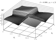
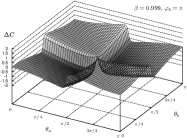
Figure 1: Function $\Delta C$ (Eq. (59)) in the parametrization $\mathbf{n}=(0,0,1)$, $\mathbf{a}=(\sin{\theta_{a}},0,\cos{\theta_{a}})$, $\mathbf{b}=(\cos{\varphi_{b}}\sin{\theta_{b}},\sin{\varphi_{b}}\sin{\theta_{b}},\cos{\theta_{b}})$. We have plotted the graph of the function $\Delta C$ for two arbitrarily chosen values of $\varphi_{b}$ and for $\beta=0.999$, which is the value for electron–positron pair created in the $\pi^{0}$ decay.

V.2 Vector state

General vector state is given by Eq. (35). So in this case from (50) we get

$$C_{{\textsf{vec}}}^{\mathcal{AB}}(\mathbf{a},\mathbf{b})=\\ \Bigg{\{}\int\frac{d^{3}\mathbf{k}}{2k^{0}}\frac{d^{3}\mathbf{p}}{2p^{0}}\chi_{\mathcal{A}}(p)\chi_{\mathcal{B}}(k)\left(\delta^{4}(q-k-p)\right)^{2}\varphi_{\mu}(k,p)\varphi_{\nu}^{*}(k,p)\text{Tr}\left[\mathbf{b}{\cdot}\boldsymbol{\sigma}\Big{(}\textsf{v}^{T}(k)\mathcal{C}\gamma^{\mu}\textsf{v}(p)\Big{)}\mathbf{a}{\cdot}\boldsymbol{\sigma}^{T}\Big{(}\textsf{v}^{T}(k)\mathcal{C}\gamma^{\nu}\textsf{v}(p)\Big{)}^{\dagger}\right]\Bigg{\}}\\ \times\Bigg{\{}\int\frac{d^{3}\mathbf{k}}{2k^{0}}\frac{d^{3}\mathbf{p}}{2p^{0}}\chi_{\mathcal{A}}(p)\chi_{\mathcal{B}}(k)\left(\delta^{4}(q-k-p)\right)^{2}\varphi_{\mu}(k,p)\varphi_{\nu}^{*}(k,p)\,\text{Tr}\left[\Big{(}\textsf{v}^{T}(k)\mathcal{C}\gamma^{\mu}\textsf{v}(p)\Big{)}\Big{(}\textsf{v}^{T}(k)\mathcal{C}\gamma^{\nu}\textsf{v}(p)\Big{)}^{\dagger}\right]\Bigg{\}}^{-1},$$ (60)

where, as before, $\chi_{\mathcal{A}}(p)$ i $\chi_{\mathcal{B}}(k)$ are characteristic functions of the regions $\mathcal{A}$ and $\mathcal{B}$ in momentum space. If the observers frame coincides with the center of mass reference frame (in which $p=k^{\pi}=(k^{0},-\mathbf{k})$) then by means of the transversality condition (37), we have

$$\varphi_{\mu}(k,k^{\pi})\varphi_{\nu}^{*}(k,k^{\pi})\text{Tr}\left[\mathbf{b}{\cdot}\boldsymbol{\sigma}\Big{(}\textsf{v}^{T}(k)\mathcal{C}\gamma^{\mu}\textsf{v}(k^{\pi})\Big{)}\mathbf{a}{\cdot}\boldsymbol{\sigma}^{T}\Big{(}\textsf{v}^{T}(k)\mathcal{C}\gamma^{\nu}\textsf{v}(k^{\pi})\Big{)}^{\dagger}\right]=\\ =\frac{2}{m^{2}}\Bigg{\{}(\mathbf{a}{\cdot}\mathbf{b})\left[{k^{0}}^{2}|\boldsymbol{\varphi}|^{2}-|\mathbf{k}{\cdot}\boldsymbol{\varphi}|^{2}\right]-{k^{0}}^{2}\left[(\mathbf{a}{\cdot}\boldsymbol{\varphi}^{*})(\mathbf{b}{\cdot}\boldsymbol{\varphi})+(\mathbf{a}{\cdot}\boldsymbol{\varphi})(\mathbf{b}{\cdot}\boldsymbol{\varphi}^{*})\right]-\frac{2(\mathbf{a}{\cdot}\mathbf{k})(\mathbf{b}{\cdot}\mathbf{k})|\mathbf{k}{\cdot}\boldsymbol{\varphi}|^{2}}{(m+k^{0})^{2}}\\ +\frac{k^{0}}{m+k^{0}}\Big{[}(\mathbf{a}{\cdot}\mathbf{k})\left((\mathbf{b}{\cdot}\boldsymbol{\varphi})(\boldsymbol{\varphi}^{*}{\cdot}\mathbf{k})+(\mathbf{b}{\cdot}\boldsymbol{\varphi}^{*})(\boldsymbol{\varphi}{\cdot}\mathbf{k})\right)+(\mathbf{b}{\cdot}\mathbf{k})\left((\mathbf{a}{\cdot}\boldsymbol{\varphi})(\boldsymbol{\varphi}^{*}{\cdot}\mathbf{k})+(\mathbf{a}{\cdot}\boldsymbol{\varphi}^{*})(\boldsymbol{\varphi}{\cdot}\mathbf{k})\right)\Big{]}\Bigg{\}}.$$ (61)

$$\varphi_{\mu}(k,k^{\pi})\varphi_{\nu}^{*}(k,k^{\pi})\text{Tr}\left[\Big{(}\textsf{v}^{T}(k)\mathcal{C}\gamma^{\mu}\textsf{v}(k^{\pi})\Big{)}\Big{(}\textsf{v}^{T}(k)\mathcal{C}\gamma^{\nu}\textsf{v}(k^{\pi})\Big{)}^{\dagger}\right]=\frac{2}{m^{2}}\Big{[}{k^{0}}^{2}|\boldsymbol{\varphi}|^{2}-|\mathbf{k}{\cdot}\boldsymbol{\varphi}|^{2}\Big{]}.$$ (62)

Therefore, if we assume that momenta of the particles in the state $\mbox{$|\varphi\rangle$}^{{\textsf{vec}}}_{q}$ are sharp, the correlation function in the center of mass frame are given by (antiparticle has momentum $k$, particle $k^{\pi}$)

$$C_{{{\textsf{vec}}}}^{{\textsf{CMF}}}(\mathbf{a},\mathbf{b})=\mathbf{a}{\cdot}\mathbf{b}-\frac{{k^{0}}^{2}}{{k^{0}}^{2}|\boldsymbol{\varphi}|^{2}-|\mathbf{k}{\cdot}\boldsymbol{\varphi}|^{2}}\left[(\mathbf{a}{\cdot}\boldsymbol{\varphi}^{*})(\mathbf{b}{\cdot}\boldsymbol{\varphi})+(\mathbf{a}{\cdot}\boldsymbol{\varphi})(\mathbf{b}{\cdot}\boldsymbol{\varphi}^{*})\right]-\frac{2(\mathbf{a}{\cdot}\mathbf{k})(\mathbf{b}{\cdot}\mathbf{k})|\mathbf{k}{\cdot}\boldsymbol{\varphi}|^{2}}{(m+k^{0})^{2}\big{(}{k^{0}}^{2}|\boldsymbol{\varphi}|^{2}-|\mathbf{k}{\cdot}\boldsymbol{\varphi}|^{2}\big{)}}\\ +\frac{k^{0}\left[(\mathbf{a}{\cdot}\mathbf{k})\left((\mathbf{b}{\cdot}\boldsymbol{\varphi})(\mathbf{k}{\cdot}\boldsymbol{\varphi}^{*})+(\mathbf{b}{\cdot}\boldsymbol{\varphi}^{*})(\mathbf{k}{\cdot}\boldsymbol{\varphi})\right)+(\mathbf{b}{\cdot}\mathbf{k})\left((\mathbf{a}{\cdot}\boldsymbol{\varphi})(\mathbf{k}{\cdot}\boldsymbol{\varphi}^{*})+(\mathbf{a}{\cdot}\boldsymbol{\varphi}^{*})(\mathbf{k}{\cdot}\boldsymbol{\varphi})\right)\right]}{(m+k^{0})\big{(}{k^{0}}^{2}|\boldsymbol{\varphi}|^{2}-|\mathbf{k}{\cdot}\boldsymbol{\varphi}|^{2}\big{)}}.$$ (63)

Notice that in this case, in opposition to the one considered previously, in the center of mass frame the correlation function depends explicitly on the momentum. Moreover, if $\mathbf{k}\perp\boldsymbol{\varphi}$ from (63) we get the same result as for nonrelativistic triplet state (86). Also in the nonrelativistic limit (${k^{0}}^{2}\gg|\mathbf{k}|^{2}$) from (63) we get the correlation function for nonrelativistic triplet state (86).

When we consider electron–positron pairs produced in the $Z^{0}$ decay two remarks are in order. First, in some experiments it is possible to produce polarized $Z^{0}$ (SLAC, Stanfordcab ), so in such experiments the vector $\boldsymbol{\varphi}$ is determined. Second, electron and positrons produced in the channel $Z^{0}\to e^{+}e^{-}$ are highly ultrarelativistic. In the limit $\beta\to 1$ the formula (63) takes the form

$$\left.C_{{{\textsf{vec}}}}^{{\textsf{CMF}}}(\mathbf{a},\mathbf{b})\right|_{\beta\to 1}=\mathbf{a}{\cdot}\mathbf{b}-\frac{1}{|\boldsymbol{\varphi}|^{2}-|\mathbf{n}{\cdot}\boldsymbol{\varphi}|^{2}}\Big{\{}(\mathbf{a}{\cdot}\boldsymbol{\varphi}^{*})(\mathbf{b}{\cdot}\boldsymbol{\varphi})+(\mathbf{a}{\cdot}\boldsymbol{\varphi})(\mathbf{b}{\cdot}\boldsymbol{\varphi}^{*})+2(\mathbf{a}{\cdot}\mathbf{n})(\mathbf{b}{\cdot}\mathbf{n})|\mathbf{n}{\cdot}\boldsymbol{\varphi}|^{2}\\ -(\mathbf{a}{\cdot}\mathbf{n})\big{[}(\mathbf{b}{\cdot}\boldsymbol{\varphi})(\mathbf{n}{\cdot}\boldsymbol{\varphi}^{*})+(\mathbf{b}{\cdot}\boldsymbol{\varphi}^{*})(\mathbf{n}{\cdot}\boldsymbol{\varphi})\big{]}-(\mathbf{b}{\cdot}\mathbf{n})\big{[}(\mathbf{a}{\cdot}\boldsymbol{\varphi})(\mathbf{n}{\cdot}\boldsymbol{\varphi}^{*})+(\mathbf{a}{\cdot}\boldsymbol{\varphi}^{*})(\mathbf{n}{\cdot}\boldsymbol{\varphi})\big{]}\Big{\}},$$ (64)

where $\mathbf{n}=\mathbf{k}/|\mathbf{k}|$. Eq. (64) takes very simple form in the configuration $\mathbf{a}\perp\boldsymbol{\varphi}$, $\mathbf{b}\perp\boldsymbol{\varphi}$:

$$\left.C_{{{\textsf{vec}}}}^{{\textsf{CMF}}}(\mathbf{a}\perp\boldsymbol{\varphi},\mathbf{b}\perp\boldsymbol{\varphi})\right|_{\beta\to 1}=\mathbf{a}{\cdot}\mathbf{b}-\frac{2(\mathbf{a}{\cdot}\mathbf{n})(\mathbf{b}{\cdot}\mathbf{n})|\mathbf{n}{\cdot}\boldsymbol{\varphi}|^{2}}{|\boldsymbol{\varphi}|^{2}-|\mathbf{n}{\cdot}\boldsymbol{\varphi}|^{2}},$$ (65)

It is interesting to notice, that the function

$$\Delta C_{{{\textsf{vec}}}}=\left.C_{{{\textsf{vec}}}}^{{\textsf{CMF}}}(\mathbf{a}\perp\boldsymbol{\varphi},\mathbf{b}\perp\boldsymbol{\varphi})\right|_{\beta\to 1}-C_{{{\textsf{nonrelativ}}}}=-\frac{2(\mathbf{a}{\cdot}\mathbf{n})(\mathbf{b}{\cdot}\mathbf{n})|\mathbf{n}{\cdot}\boldsymbol{\varphi}|^{2}}{|\boldsymbol{\varphi}|^{2}-|\mathbf{n}{\cdot}\boldsymbol{\varphi}|^{2}},$$ (66)

where $C_{{{\textsf{nonrelativ}}}}$ denotes correlation function for the nonrelativistic triplet state (86), can take arbitrary value from the interval $[-2,2]$. We shown this function in the Fig. 2.

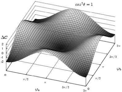
Figure 2: Function $\Delta C$ (Eq. (66)) in the parametrization $\boldsymbol{\varphi}=(0,0,1)$, $\mathbf{n}=(\sin\theta,0,\cos\theta)$, $\mathbf{a}=(\cos{\varphi_{a}},\sin{\varphi_{a}},0)$, $\mathbf{b}=(\cos{\varphi_{b}},\sin{\varphi_{b}},0)$. In this parametrization $\Delta C=-2\cos{\varphi_{a}}\cos{\varphi_{b}}\cos^{2}\theta$. We have plotted the graph for the value $\theta$ such that $\cos^{2}\theta=1$. We see that $\Delta C$ is of the same order of magnitude as the correlation function.

VI Conclusions

We have discussed correlations of two relativistic massive particles in the EPR–type experiments in the context of quantum field theory formalism. Choosing the most appropriate spin operator (38), we have calculated correlation function for the particle–anti–particle pair in the pseudoscalar and vector states. We have found general formulas and discussed them in some details for the sharp momentum states in the specific configurations. Relativistic correlations in the vector state have been never discussed before. It should also be noted that all these functions posses a proper nonrelativistic limit.

It is interesting that for the pseudoscalar (singlet) state the correlation function in the center of mass frame is the same as in the nonrelativistic case. Therefore, in opposition to Czachor’s results Czachor (1997a), the degree of violation of Bell inequality for the pseudoscalar state in CMF is independent of the particle momentum. The correlation function for the vector state depends on the configuration and for same configurations gives the same result as for the nonrelativistic triplet state.

It seems that EPR–type experiment with relativistic elementary particles are feasible with the present technology Ciborowski .

Appendix A Dirac matrices

In this paper we use the following conventions. Dirac matrices fulfill the relation $\gamma^{\mu}\gamma^{\nu}+\gamma^{\nu}\gamma^{\mu}=2g^{\mu\nu}$ where the Minkowski metric tensor $g^{\mu\nu}=\text{diag}(1,-1,-1,-1)$; moreover we adopt the convention $\varepsilon^{0123}=1$. We use the following explicit representation of gamma matrices:

$$\gamma^{0}=\left(\begin{array}[]{cc}0&I\\ I&0\end{array}\right),\quad{\boldsymbol{\gamma}}=\left(\begin{array}[]{cc}0&-{\boldsymbol{\sigma}}\\ {\boldsymbol{\sigma}}&0\end{array}\right),\quad\gamma^{5}=\left(\begin{array}[]{cc}I&0\\ 0&-I\end{array}\right),$$ (67)

where $\boldsymbol{\sigma}=(\sigma_{1},\sigma_{2},\sigma_{3})$ and $\sigma_{i}$ are standard Pauli matrices. The charge conjugation matrix has the form

$$\mathcal{C}=-i\gamma^{2}\gamma^{0}=i\left(\begin{smallmatrix}\sigma_{2}&0\\ 0&-\sigma_{2}\end{smallmatrix}\right),$$ (68)

so

$$\mathcal{C}\gamma^{T\mu}\mathcal{C}^{-1}=-\gamma^{\mu}.$$ (69)

Appendix B Bispinor representation

By the bispinor representation of the Lorentz group we mean the representation $D^{(\frac{1}{2},0)}\oplus D^{(0,\frac{1}{2})}$. Explicitly, if $A\in SL(2,{\mathbb{C}})$ and $\Lambda(A)$ is an image of $A$ in the canonical homomorphism of the $SL(2,{\mathbb{C}})$ group onto the Lorentz group, we take the chiral form of $D^{(\frac{1}{2},0)}\oplus D^{(0,\frac{1}{2})}$, namely

$$\textsf{D}(\Lambda(A))=\begin{pmatrix}A&0\\ 0&(A^{\dagger})^{-1}\end{pmatrix}.$$ (70)

The canonical homomorphism between the group $SL(2,{\mathbb{C}})$ (universal covering of the proper ortochronous Lorentz group $L_{+}^{\uparrow}$) and the Lorentz group $L_{+}^{\uparrow}\sim SO(1,3)_{0}$ Barut and Ra̧czka (1977) is defined as follows: With every four-vector $k^{\mu}$ we associate a two-dimensional hermitian matrix $k^{\mu}\sigma_{\mu}$, where $\sigma_{i}$, $i=1,2,3$, are the standard Pauli matrices and $\sigma_{0}=I$. In the space of two-dimensional hermitian matrices the Lorentz group action is given by ${{\sf k}^{\prime}}^{\mu}\sigma_{\mu}=A({\textsf{k}}^{\mu}\sigma_{\mu})A^{\dagger}$, where $A$ denotes the element of the $SL(2,{\mathbb{C}})$ group corresponding to the Lorentz transformation $\Lambda(A)$ which converts the four-vector $k$ to $k^{\prime}$ (i.e., ${k^{\prime}}^{\mu}=\Lambda_{\phantom{\mu}\nu}^{\mu}k^{\nu}$).

Appendix C Useful formulas

The following relations hold:

$$(k\gamma)\,\textsf{v}(k)=m\textsf{v}(k),$$ (71)

$$\bar{\textsf{v}}(k)\textsf{v}(k)=I,$$ (72)

$$\gamma^{0}\textsf{v}(k)=\textsf{v}(k^{\pi}),$$ (73)

$$\bar{\textsf{v}}(k)\gamma^{\mu}\textsf{v}(k)=\frac{k^{\mu}}{m}I,$$ (74)

$$\textsf{v}(k)\bar{\textsf{v}}(k)=\tfrac{1}{2m}(k\gamma+mI),$$ (75)

and

$$\textsf{v}(\Lambda k)=\textsf{D}(\Lambda)\textsf{v}(k)\mathcal{D}^{T}(R(\Lambda,k)),$$ (76)

$$\textsf{v}(\Lambda k)\sigma_{2}=\textsf{D}(\Lambda)\,\textsf{v}(k)\sigma_{2}\,\mathcal{D}^{\dagger}(R(\Lambda,k)).$$ (77)

Notice that when operator $\hat{A}$ acts on standard basis vectors in the following way

$$\hat{A}\mbox{$|k,\sigma\rangle$}=A_{\sigma\sigma^{\prime}}\mbox{$|k,\sigma^{\prime}\rangle$},$$ (78)

then its action on the covariant basis (18) is of the form

$$\hat{A}\mbox{$|\alpha,k\rangle$}=\left(\textsf{v}(k)A\bar{\textsf{v}}(k)\right)_{\alpha\alpha^{\prime}}\mbox{$|\alpha^{\prime},k\rangle$}.$$ (79)

Analogously for two–particle states the relation

$$(\hat{A}\otimes\hat{B})\mbox{$|(k,\sigma)_{b},(p,\lambda)_{a}\rangle$}=A_{\sigma\sigma^{\prime}}B_{\lambda\lambda^{\prime}}\mbox{$|(k,\sigma^{\prime})_{b},(p,\lambda^{\prime})_{a}\rangle$}$$ (80)

implies

$$(\hat{A}\otimes\hat{B})\mbox{$|(\alpha,k),(\beta,p)\rangle$}=\left(\textsf{v}(k)\hat{A}\bar{\textsf{v}}(k)\right)_{\alpha\alpha^{\prime}}\\ \left(\textsf{v}(p)\hat{B}\bar{\textsf{v}}(p)\right)_{\beta\beta^{\prime}}\mbox{$|(\alpha^{\prime},k),(\beta^{\prime},p)\rangle$}.$$ (81)

Appendix D Correlations in nonrelativistic triplet state

We recall in this appendix the correlation function in nonrelativistic triplet state (see e.g. Caban et al. (2003)). Let $|\sigma\rangle$, $\sigma=\pm\frac{1}{2}$, denotes eigenvector of the spin component along $z$ axis corresponding to the value of spin z–component equal to $\sigma$. The general triplet state has the form

$$\mbox{$|\varphi\rangle$}=\sum\limits_{\sigma,\lambda=\pm 1/2}\varphi_{\sigma\lambda}\mbox{$|\sigma\rangle$}\otimes\mbox{$|\lambda\rangle$},$$ (82)

with the symmetry condition

$$\varphi_{\sigma\lambda}=\varphi_{\lambda\sigma}.$$ (83)

It is convenient to parametrize matrix $\varphi=[\varphi_{\sigma\lambda}]$ in the following way:

$$\varphi=\frac{i}{\sqrt{2}}({\boldsymbol{\varphi}}{\cdot}{\boldsymbol{\sigma}})\sigma_{2}.$$ (84)

So finally the normalized correlation function in the triplet state is given by

$$C(\mathbf{a},\mathbf{b}) = \mbox{$\langle\varphi|$}\mathbf{a}{\cdot}{\boldsymbol{\sigma}}\otimes\mathbf{b}{\cdot}{\boldsymbol{\sigma}}\mbox{$|\varphi\rangle$}$$ (85)

$$= \mathbf{a}{\cdot}\mathbf{b}-\frac{1}{|{\boldsymbol{\varphi}}|^{2}}[(\mathbf{a}{\cdot}{\boldsymbol{\varphi}})(\mathbf{b}{\cdot}{\boldsymbol{\varphi}}^{*})+(\mathbf{b}{\cdot}{\boldsymbol{\varphi}})(\mathbf{a}{\cdot}{\boldsymbol{\varphi}}^{*})].$$ (86)

References

- Einstein et al. (1935) A. Einstein, B. Podolsky, and N. Rosen, Phys. Rev. 47, 777 (1935).
- Rove et al. (2001) M. A. Rove, D. Kielpinski, V. Meyer, C. A. Sackett, W. M. Itano, C. Monroe, and D. J. Wineland, Nature 409, 781 (2001).
- Weihs et al. (1998) G. Weihs, T. Jennewein, C. Simon, H. Weinfurter, and A. Zeilinger, Phys. Rev. Lett. 81, 5039 (1998).
- Czachor (1997a) M. Czachor, Phys. Rev. A 55, 72 (1997a).
- Czachor (1997b) M. Czachor, in Photonic Quantum Computing, edited by S. P. Holating and A. R. Pirich (SPIE - The International Society for Optical Engineering, Bellingham, WA, 1997b), vol. 3076 of Proceedings of SPIE, pp. 141–145.
- Ahn et al. (2002) D. Ahn, H. J. Lee, and S. W. Hwang (2002), eprint arXiv: quant-ph/0207018.
- Ahn et al. (2003a) D. Ahn, H. J. Lee, S. W. Hwang, and M. S. Kim (2003a), eprint arXiv: quant-ph/0304119.
- Ahn et al. (2003b) D. Ahn, H. J. Lee, Y. H. Moon, and S. W. Hwang, Phys. Rev. A 67, 012103 (2003b).
- Alsing and Milburn (2002) P. M. Alsing and G. J. Milburn, Q. Inf. and Comput. 2, 487 (2002).
- Bartlett and Terno (2005) S. D. Bartlett and D. R. Terno, Phys. Rev. A 71, 012302 (2005).
- Caban and Rembieliński (2003) P. Caban and J. Rembieliński, Phys. Rev. A 68, 042107 (2003).
- Caban and Rembieliński (2005) P. Caban and J. Rembieliński, Phys. Rev. A 72, 012103 (2005).
- Czachor and Wilczewski (2003) M. Czachor and M. Wilczewski, Phys. Rev. A 68, 010302(R) (2003).
- Czachor (2005) M. Czachor, Phys. Rev. Lett. 94, 078901 (2005).
- Gingrich and Adami (2002) R. M. Gingrich and C. Adami, Phys. Rev. Lett. 89, 270402 (2002).
- Gingrich et al. (2003) R. M. Gingrich, A. J. Bergou, and C. Adami, Phys. Rev. A 68, 042102 (2003).
- Gonera et al. (2004) C. Gonera, P. Kosiński, and P. Maślanka, Phys. Rev. A 70, 034102 (2004).
- Harshman (2005) N. L. Harshman, Phys. Rev. A 71, 022312 (2005).
- Jordan et al. (2005) T. F. Jordan, A. Shaji, and E. C. G. Sudarshan, Phys. Rev. A 73, 032104 (2005).
- Kosiński and Maślanka (2003) P. Kosiński and P. Maślanka (2003), eprint arXiv: quant-ph/0310145.
- Lamata et al. (2005) L. Lamata, M. A. Martin-Delgado, and E. Solano (2005), eprint arXiv: quant-ph/051208.
- Lee and Chang-Young (2004) D. Lee and E. Chang-Young, New J. Phys. 6, 67 (2004).
- Li and Du (2003) H. Li and J. Du, Phys. Rev. A 68, 022108 (2003).
- Li and Du (2004) H. Li and J. Du, Phys. Rev. A 70, 012111 (2004).
- Lindner et al. (2003) N. H. Lindner, A. Peres, and D. R. Terno, J. Phys. A: Math. Gen. 36, L449 (2003).
- Moon et al. (2003) Y. H. Moon, D. Ahn, and S. W. Hwang (2003), eprint arXiv: quant-ph/0304116.
- Peres et al. (2002) A. Peres, P. F. Scudo, and D. R. Terno, Phys. Rev. Lett. 88, 230402 (2002).
- Peres and Terno (2003a) A. Peres and D. R. Terno, J. Mod. Optics 50, 1165 (2003a).
- Peres and Terno (2003b) A. Peres and D. R. Terno, Int. J. Q. Inf. 1, 225 (2003b).
- Peres and Terno (2004) A. Peres and D. R. Terno, Rev. Mod. Phys. 76, 93 (2004).
- Peres et al. (2005) A. Peres, P. F. Scudo, and D. R. Terno, Phys. Rev. Lett. 94, 078902 (2005).
- Pachos and Solano (2003) J. Pachos and E. Solano, Q. Inf. and Comput. 3, 115 (2003).
- Rembieliński and Smoliński (2002) J. Rembieliński and K. A. Smoliński, Phys. Rev. A 66, 052114 (2002).
- Soo and Lin (2004) C. Soo and C. C. Y. Lin, Int. J. Q. Inf. 2, 183 (2004).
- Terashima and Ueda (2003a) H. Terashima and M. Ueda, Int. J. Q. Inf. 1, 93 (2003a).
- Terashima and Ueda (2003b) H. Terashima and M. Ueda, Q. Inf. and Comput. 3, 224 (2003b).
- Terno (2003) D. R. Terno, Phys. Rev. A 67, 014102 (2003).
- Terno (2005) D. R. Terno (2005), eprint arXiv: quant-ph/0508049.
- Timpson and Brown (2002) C. G. Timpson and H. R. Brown, in Understending Physical Knowlwdge, edited by R. Lupacchini and V. Fano (Department of Philosophy, University of Bologna, CLUEB, 2002).
- You et al. (2004) H. You, A. M. Wang, X. Young, W. Niu, X. Ma, and F. Xu, Phys. Lett. A 333, 389 (2004).
- Zbinden et al. (2001) H. Zbinden, J. Brendel, N. Gisin, and W. Tittel, Phys. Rev. A 63, 022111 (2001).
- Jordan et al. (2006) T. F. Jordan, A. Shaji, and E. C. G. Sudarshan, Lorentz transformations that entangle spins and entangle momenta (2006), eprint arXiv: quant-ph/0608061.
- Kim and Son (2005) W. T. Kim and E. J. Son, Phys. Rev. A 71, 014102 (2005).
- Lamehi-Rachti and Mittig (1976) M. Lamehi-Rachti and W. Mittig, Phys. Rev. D 14, 2543 (1976).
- Eidelman et al. (2004) S. Eidelman, K. G. Hayes, K. A. Olive, M. Aguilar-Benitez, C. Amsler, D. Asner, and at al, Phys. Lett. B 592, 1 (2004).
- Bogolubov et al. (1975) N. N. Bogolubov, A. A. Logunov, and I. T. Todorov, Introduction to Axiomatic Quantum Field Theory (W. A. Benjamin, Reading, Mass., 1975).
- (47) URL http://www-sld.slac.stanford.edu/sldwww/pubs.html.
- (48) J. Ciborowski, private communication.
- Barut and Ra̧czka (1977) A. O. Barut and R. Ra̧czka, Theory of Group Representations and Applications (PWN, Warszawa, 1977).
- Caban et al. (2003) P. Caban, J. Rembieliński, K. A. Smoliński, and Z. Walczak, Phys. Rev. A 67, 012109 (2003).
- Caban and Rembieliński (1999) P. Caban and J. Rembieliński, Phys. Rev. A 59, 4187 (1999).