Photon number states generated from a continuous-wave light source

Abstract

Conditional preparation of photon number states from a continuous-wave nondegenerate optical parametric oscillator is investigated. We derive the phase space Wigner function for the output state conditioned on photo detection events that are not necessarily simultaneous, and we maximize its overlap with the desired photon number state by choosing the optimal temporal output state mode function. We present a detailed numerical analysis for the case of two-photon state generation from a parametric oscillator driven with an arbitrary intensity below threshold, and in the low intensity limit, we present a formalism that yields the optimal output state mode function and fidelity for higher photon number states.

I Introduction

The study of nonclassical states of light has provided a deeper understanding of quantum fluctuations and the role of measurements in quantum theory and it has led to applications in precision metrology and quantum communication. The photon number states, or Fock states, play a special role, because they have vanishing intensity fluctuations, and their interaction, e.g., with a single two-level atom in an optical cavity, is particularly regular. By injection of atoms with properly selected excitation and passage times through a micro maser, it is possible to build up a wide range of states, including number states of the cavity field walther ; haroche , and recent progress in extending the photon lifetimes in microwave cavities harochenature bring promise for further experimental progress in this direction.

By control of single photo emitters such as a single molecule molecule , a color center colorcenter , or a quantum dot dot , it is also possible to generate traveling light pulses in the optical frequency range that contain only a single photon. For a review on single photon emitters see singlereview . In these schemes, however, the production of higher number states is not straightforward, and in the present paper we shall address an alternative conditional approach where the signal beam from a nondegenerate optical parametric oscillator (OPO) is projected into the desired state by a quantum measurement performed on the idler beam. This method has recently been used to generate single- and two-photon states from an OPO driven by a pulsed pump field grangier2 . Conditional generation of nonclassical states was proposed by Dakna et al dakna , see also kim ; fiurasek , and generation of single-photon and Schrödinger cat states has been demonstrated in experiments where measurements performed on a small fraction of the light beam from a degenerate OPO caused the projection of the remaining beam grangiercat ; jonas ; wakui . Single-photon and cat state production from continuous-wave OPOs has been studied theoretically in sasaki ; klaus ; nm , and in the present paper we generalize the analysis to continuous-wave generation of higher photon number states. In contrast to single photon and Schrödinger cat state production, generation of states with two or more photons involves multiple conditioning photo detection events, and in the continuous-wave case, we are particularly interested in determining how the generated state is affected by the temporal separation of the conditioning detections. We analyze this feature generally for two-photon states and we present an analytical treatment, restricted to the low intensity limit, for $n$-photon state generation.

Figure 1 exemplifies the experimental setup used to generate Fock states. A nondegenerate OPO produces pairs of distinguishable photons. The two kinds of photons are separated to produce two correlated twin beams. One beam (denoted the trigger) is observed with an avalanche photodiode (APD) detector. Detection of $n$ close detector clicks in the trigger arm projects the state in the signal beam into an $n$-photon state, and the generation is verified by homodyne detection. Since the field is a continuous-wave field the temporal mode occupied by the produced state needs to be specified, and the largest $n$-photon fidelities are obtained by optimizing the choice of signal state mode function. We shall investigate to which extent the $n$ photons in the signal beam may occupy a single mode despite the click events happening not exactly simultaneously.

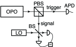
Figure 1: Experimental setup for conditional preparation of Fock states from a type II (i.e. polarization) nondegenerate OPO. PBS: polarizing beam splitter, APD: avalanche photodiode, BS: beam splitter, and LO: local oscillator.

In order not to miss close clicks due to the finite dead time of real detectors it might be advantageous to split the trigger beam and send it onto more than one APD detector, as was done in the two-photon experiment with pulsed fields grangier2 . However, we show that our theoretical expression for the conditional output state, and thus also the fidelity and the optimal signal state mode function, is independent of the number of (ideal) APD detectors used.

In Sec. II we start out with a two-mode treatment of the two-photon state generation process. In Sec. III we generalize to the multi-mode case valid for continuous-wave fields. We determine the Wigner function for the output state conditioned on two trigger detector click events, and we calculate the two-photon state fidelity as a function of the signal state mode function. In Sec. IV we optimize the signal state mode function over all real functions to obtain maximal two-photon state fidelity. Finally, in Sec. V, we consider $n$-photon state generation in the low intensity limit. We describe the state produced in the signal beam in terms of photons occupying specific temporal modes, and we determine the optimal output state mode functions. Sec. VI concludes the paper.

II Output state conditioned on two trigger detector click events – two-mode treatment

In this section we describe the two-photon state generation in the context of a simple two-mode theory to introduce some of the basic ideas. This treatment is approximately valid when a pulsed pump field is used. The initial state generated by the nondegenerate OPO is a two-mode squeezed vacuum state ban

$$|\psi_{i}\rangle=\frac{1}{\cosh(r)}\sum_{n=0}^{\infty}\tanh^{n}(r)|n,n\rangle,$$ (1)

where $r$ is the squeezing parameter and the first (second) quantum number inside the ket on the right hand side is the number of photons in the trigger (signal) mode.

We assume that a trigger detector click results in the transformation $\rho\rightarrow\hat{a}_{t}\rho\hat{a}^{\dagger}_{t}/\mathrm{Tr}(\hat{a}_{t}\rho\hat{a}^{\dagger}_{t})$ of the density operator $\rho$, where $\hat{a}_{t}$ is the trigger mode annihilation operator. We apply the click transformation twice to the state (1), and since we do not subject the trigger mode to further measurements, we trace over the trigger mode afterward and renormalize to obtain the conditional single-mode output state

$$\rho_{click}=\\ \frac{1}{2\cosh^{2}(r)\sinh^{4}(r)}\sum_{n=0}^{\infty}\tanh^{2n}(r)n(n-1)|n\rangle\langle n|.$$ (2)

The vacuum and the single-photon state contributions are eliminated by the conditioning procedure, and the generated state is a superposition of a two-photon state and higher photon number states. The two-photon state fidelity is easily obtained from (2) as

$$F_{2}=\langle 2|\rho_{click}|2\rangle=\frac{1}{\cosh^{6}(r)}.$$ (3)

The fidelity approaches unity in the limit where the squeezing parameter is small, because a small $r$ corresponds to a weak pump field, and hence the probability to produce more than two photon pairs within a single pulse is small.

For the multi-mode case it turns out to be convenient to describe the initial unconditional state and the conditional state in terms of Wigner functions, and we hence introduce this alternative approach now. Since the OPO is a Gaussian light source, the two-mode Wigner function for the initial unconditional state is a Gaussian

$$W_{V}(y)=\frac{1}{\pi^{2}\sqrt{\det(V)}}\exp\left(-y^{T}V^{-1}y\right).$$ (4)

$y=(x_{t},p_{t},x_{s},p_{s})^{T}$ is a column vector of quadrature variables for the trigger and the signal mode, and $V$ is the covariance matrix. In terms of the operators $\hat{y}=(\hat{x}_{t},\hat{p}_{t},\hat{x}_{s},\hat{p}_{s})^{T}$, defined as $\hat{x}_{t/s}=(\hat{a}_{t/s}+\hat{a}^{\dagger}_{t/s})/\sqrt{2}$, and $\hat{p}_{t/s}=-i(\hat{a}_{t/s}-\hat{a}^{\dagger}_{t/s})/\sqrt{2}$, where $\hat{a}_{s}$ is the annihilation operator for the signal mode, the elements of the covariance matrix are $V_{ij}=\langle\hat{y}_{i}\hat{y}_{j}\rangle+\langle\hat{y}_{j}\hat{y}_{i}\rangle$, and from (1) we obtain

$$V_{11}=V_{22} = V_{33}=V_{44}=\cosh(2r),$$ (5)

$$V_{13}=V_{31} = -V_{24}=-V_{42}=\sinh(2r),$$ (6)

while the other matrix elements are zero.

The transformation from (1) to (2) is translated into (see klaus ; nm )

$$W_{click}(x_{s},p_{s})=N_{click}\iint\frac{1}{4}\bigg{(}1+x_{t}^{2}+p_{t}^{2}+x_{t}\frac{\partial}{\partial x_{t}}\\ +p_{t}\frac{\partial}{\partial p_{t}}+\frac{1}{4}\frac{\partial^{2}}{\partial x_{t}^{2}}+\frac{1}{4}\frac{\partial^{2}}{\partial p_{t}^{2}}\bigg{)}^{2}W_{V}(y)dx_{t}dp_{t}\\ =\frac{1}{\pi\cosh^{3}(2r)}\bigg{(}1-2\frac{1+\cosh(2r)}{\cosh(2r)}\left(x_{s}^{2}+p_{s}^{2}\right)\\ +\frac{[1+\cosh(2r)]^{2}}{2\cosh^{2}(2r)}\left(x_{s}^{2}+p_{s}^{2}\right)^{2}\bigg{)}\exp\left(-\frac{x_{s}^{2}+p_{s}^{2}}{\cosh(2r)}\right),$$ (7)

where $N_{click}$ is a normalization constant. The two-photon state fidelity of the generated state is given by

$$F_{2}\equiv 2\pi\iint W_{click}(x_{s},p_{s})W_{n=2}(x_{s},p_{s})dx_{s}dp_{s},$$ (8)

where $W_{n=2}$ is the Wigner function for a two-photon state. Equation (8) once again leads to the result (3).

III Output state conditioned on two trigger detector click events – multi-mode treatment

In the continuous-wave case the field annihilation operators are time-dependent and satisfy the commutator relation $[\hat{a}(t),\hat{a}^{\dagger}(t^{\prime})]=\delta(t-t^{\prime})$. In the following we denote the trigger beam annihilation operator $\hat{a}_{+}(t)$ and the signal beam annihilation operator $\hat{a}_{-}(t)$ to distinguish them from the single mode operators in the last section. In principle, there are now infinitely many modes, but since we can trace out all unobserved modes, we only need to consider the two trigger modes, in which the conditioning trigger detector clicks occur, and the signal mode occupied by the generated state, which is a great simplification. It is necessary to include two trigger modes since the conditioning clicks may happen at different times. Initially we assume that the trigger modes are distinct.

The temporal shapes of the relevant modes are given by the mode functions $f_{i}(t)$, $i=1,2,3$, where 1 and 2 are trigger modes while 3 is the signal mode. The single-mode operators (corresponding to $\hat{a}_{t}$ and $\hat{a}_{s}$) are then given by

$$\hat{a}_{i} = \int f_{i}(t^{\prime})\hat{a}_{+}(t^{\prime})dt^{\prime},\quad i=1,2,$$ (9)

$$\hat{a}_{3} = \int f_{3}(t^{\prime})\hat{a}_{-}(t^{\prime})dt^{\prime}.$$ (10)

$[\hat{a}_{i},\hat{a}^{\dagger}_{i}]=1$ implies that $\int|f_{i}(t^{\prime})|^{2}dt^{\prime}=1$. We assume that the trigger modes are top hat functions of infinitesimal width $\Delta t_{c}$ and height $1/\sqrt{\Delta t_{c}}$ centered at the $i$th detection time $t_{ci}$. This is valid if the duration of a detection is much smaller than the inverse of the leakage rate $\gamma$ of the OPO output mirror. The signal mode function is used to specify the output state, and hence it may be chosen arbitrarily. In Sec. IV we use this freedom to maximize the two-photon state fidelity. We assume throughout the two-photon state analysis that the signal mode function is real. Imperfect detection may be taken into account by replacing $\hat{a}_{\pm}(t)$ with $\sqrt{\eta_{t/s}}\hat{a}_{\pm}(t^{\prime})+\sqrt{1-\eta_{t/s}}\hat{a}_{\pm,vac}(t^{\prime})$ in equations (9) and (10), where $\eta_{t/s}$ is the trigger/signal detector efficiency and $\hat{a}_{\pm,vac}$ are field operators acting on vacuum.

With the single mode operators established we proceed as in the second part of the last section, but since three modes are now included, the covariance matrix $V$ is $6\times 6$, $y=(x_{1},p_{1},x_{2},p_{2},x_{3},p_{3})^{T}$, and $\pi^{2}$ is replaced by $\pi^{3}$ in Eq. (4). To calculate the covariance matrix elements in terms of $f_{3}(t)$, $\eta_{t}$, $\eta_{s}$, and OPO parameters we need the two-time correlation functions for the nondegenerate OPO output. These are drummond

$$\langle\hat{a}_{\pm}(t)\hat{a}_{\mp}(t^{\prime})\rangle = \frac{\lambda^{2}-\mu^{2}}{4}\left(\frac{\mathrm{e}^{-\mu|t-t^{\prime}|}}{2\mu}+\frac{\mathrm{e}^{-\lambda|t-t^{\prime}|}}{2\lambda}\right),$$

$$\langle\hat{a}^{\dagger}_{\pm}(t)\hat{a}_{\pm}(t^{\prime})\rangle = \frac{\lambda^{2}-\mu^{2}}{4}\left(\frac{\mathrm{e}^{-\mu|t-t^{\prime}|}}{2\mu}-\frac{\mathrm{e}^{-\lambda|t-t^{\prime}|}}{2\lambda}\right),$$

$$\langle\hat{a}_{\pm}(t)\hat{a}_{\pm}(t^{\prime})\rangle = \langle\hat{a}^{\dagger}_{\pm}(t)\hat{a}_{\mp}(t^{\prime})\rangle=0,$$ (11)

where $\lambda=\frac{\gamma}{2}+\epsilon$, $\mu=\frac{\gamma}{2}-\epsilon$, $\epsilon$ is the nonlinear gain coefficient of the OPO, and $\gamma$ is the OPO output mirror leakage rate introduced above. Note that the dimension less twin beam intensity $\langle\hat{a}^{\dagger}_{\pm}(t)\hat{a}_{\pm}(t)\rangle/\gamma$ is an increasing function of $\epsilon/\gamma$.

In analogy to Eq. (7) the single-mode Wigner function for the state conditioned on two trigger detector clicks is

$$W_{click}(x_{3},p_{3})=N_{click}\int\prod_{i=1}^{2}\bigg{[}dx_{i}dp_{i}\frac{1}{2}\bigg{(}1+x_{i}^{2}+p_{i}^{2}\\ +x_{i}\frac{\partial}{\partial x_{i}}+p_{i}\frac{\partial}{\partial p_{i}}+\frac{1}{4}\frac{\partial^{2}}{\partial x_{i}^{2}}+\frac{1}{4}\frac{\partial^{2}}{\partial p_{i}^{2}}\bigg{)}\bigg{]}W_{V}(y)\\ =\frac{1}{C_{1}}\big{[}C_{2}+C_{3}(x_{3}^{2}+p_{3}^{2})+C_{4}(x_{3}^{2}+p_{3}^{2})^{2}\big{]}\mathrm{e}^{-C_{5}(x_{3}^{2}+p_{3}^{2})},$$ (12)

where $C_{1}=D_{1}V_{55}\pi$, $C_{2}=D_{1}-V_{55}D_{2}$, $C_{3}=D_{2}-2V_{55}V_{15}^{2}V_{35}^{2}$, $C_{4}=V_{15}^{2}V_{35}^{2}$, $C_{5}=(V_{55})^{-1}$, and

$$D_{1} = V_{55}^{4}\left[(V_{11}-1)(V_{33}-1)+V_{13}^{2}\right],$$

$$D_{2} = V_{55}\big{\{}2V_{15}V_{35}\left(V_{13}V_{55}-V_{15}V_{35}\right)$$

$$+V_{55}\left[V_{15}^{2}(V_{33}-1)+V_{35}^{2}(V_{11}-1)\right]\big{\}}.$$

$W_{click}$ is independent of $\eta_{t}$.

If the trigger beam is divided into $m$ beams, the field operator representing the field in the $j$th beam may be written as $c_{j0}\hat{a}_{+}(t)+\sum_{i=1}^{m-1}c_{ji}\hat{a}_{i,vac}(t)$, where $c_{ji}$ are coefficients determined from the precise arrangement of beam splitters, and $\hat{a}_{i,vac}(t)$ are field operators representing vacuum states. If a click is observed in the $j$th and the $k$th trigger beam in the temporal modes $f_{1}(t)$ and $f_{2}(t)$, respectively, and we trace over all modes except the output mode (denoted by $\mathrm{Tr}^{\prime}$), the density operator $\rho_{tot}$ is transformed into

$$\rho_{tot}\rightarrow\mathrm{Tr}^{\prime}\Bigg{[}\int f_{1}(t)\left(c_{j0}\hat{a}_{+}(t)+\sum_{i=1}^{m-1}c_{ji}\hat{a}_{i,vac}(t)\right)dt\\ \int f_{2}(t^{\prime})\left(c_{k0}\hat{a}_{+}(t^{\prime})+\sum_{i=1}^{m-1}c_{ki}\hat{a}_{i,vac}(t^{\prime})\right)dt^{\prime}\\ \rho_{tot}\int f_{2}(t^{\prime\prime})\left(c^{*}_{k0}\hat{a}^{\dagger}_{+}(t^{\prime\prime})+\sum_{i=1}^{m-1}c^{*}_{ki}\hat{a}^{\dagger}_{i,vac}(t^{\prime\prime})\right)dt^{\prime\prime}\\ \int f_{1}(t^{\prime\prime\prime})\left(c^{*}_{j0}\hat{a}^{\dagger}_{+}(t^{\prime\prime\prime})+\sum_{i=1}^{m-1}c^{*}_{ji}\hat{a}^{\dagger}_{i,vac}(t^{\prime\prime\prime})\right)dt^{\prime\prime\prime}\Bigg{]},$$ (13)

where a normalization factor is omitted. The density operator $\rho_{tot}$ is the direct product of the density operator for the OPO output and the density operators for the vacuum states coupled into the system via the beam splitters. Since the annihilation operator acting on a vacuum state is zero, (13) simplifies to

$$\rho_{tot}\rightarrow\mathrm{Tr}_{12}\Bigg{[}\int f_{1}(t)c_{j0}\hat{a}_{+}(t)dt\int f_{2}(t^{\prime})c_{k0}\hat{a}_{+}(t^{\prime})dt^{\prime}\\ \rho_{123}\int f_{2}(t^{\prime\prime})c^{*}_{k0}\hat{a}^{\dagger}_{+}(t^{\prime\prime})dt^{\prime\prime}\int f_{1}(t^{\prime\prime\prime})c^{*}_{j0}\hat{a}^{\dagger}_{+}(t^{\prime\prime\prime})dt^{\prime\prime\prime}\Bigg{]},$$ (14)

where the trace is now over the two trigger modes, and $\rho_{123}$ is the density operator for the two trigger modes and the output mode. The factor $c_{j0}c_{k0}c^{*}_{k0}c^{*}_{j0}$ is irrelevant because the transformed density operator has to be normalized. The conditional output state is thus independent of the trigger detector configuration, and it is justified to use the simple setup in figure 1 in a theoretical treatment. One can verify that the Wigner function of the conditional state continuously approaches the outcome of a two-photon detection in a single trigger mode, when the click separation approaches zero. The arguments are immediately generalized to the case of $n$ conditioning clicks.

Finally, the two-photon state fidelity of the produced state is obtained from the conditional Wigner function $W_{click}$ as in Eq. (8)

$$F_{2}(f_{3}(t))=\frac{2}{D_{1}(1+V_{55})^{5}}\big{\{}D_{1}(1-V_{55})^{2}(1+V_{55})^{2}\\ -D_{2}V_{55}^{2}(1-V_{55})(1+V_{55})(5-V_{55})\\ +2V_{55}^{3}(V_{15}V_{35})^{2}[4V_{55}-5(1-V_{55})^{2}]\big{\}}.$$ (15)

The fidelity depends on the choice of signal mode function $f_{3}(t)$. In the next section we first determine the optimal mode function $f_{op}(t)$, which leads to the largest fidelity, and then we present explicit results for the predictions of equation (15).

IV Optimal signal mode function and two-photon state fidelity

In the low intensity limit (15) reduces to

$$\lim_{\epsilon\rightarrow 0}F_{2}(f_{3}(t))=\frac{V_{15}^{2}V_{35}^{2}}{2\left[(V_{11}-1)(V_{33}-1)+V_{13}^{2}\right]},$$ (16)

and for small $\epsilon/\gamma$

$$V_{15} = 2\epsilon\sqrt{\Delta t_{c}\eta_{t}\eta_{s}}\int f_{3}(t^{\prime})\mathrm{e}^{-\frac{\gamma}{2}|t^{\prime}-t_{c1}|}dt^{\prime},$$ (17)

$$V_{35} = 2\epsilon\sqrt{\Delta t_{c}\eta_{t}\eta_{s}}\int f_{3}(t^{\prime})\mathrm{e}^{-\frac{\gamma}{2}|t^{\prime}-t_{c2}|}dt^{\prime},$$ (18)

while $V_{11}$, $V_{33}$, and $V_{13}$ are always independent of $f_{3}(t)$. The optimal signal mode function at very low intensity is thus easily obtained by optimization of $V_{15}V_{35}$ under the constraint $\int f_{op}(t)^{2}dt=1$. This leads to

$$\lim_{\epsilon\rightarrow 0}f_{op}(t)=N\bigg{[}\exp\left(-\frac{\gamma}{2}|t-t_{c1}|\right)\\ +\exp\left(-\frac{\gamma}{2}|t-t_{c2}|\right)\bigg{]},$$ (19)

where $N$ is a normalization constant.

For larger intensities the fidelity can be optimized numerically by varying the shape of the mode function until no further increase in fidelity is obtained. Optimized mode functions for $|t_{c2}-t_{c1}|\gamma=4$ and different intensities are shown in figure 2. The peaks of the mode functions become sharper with increasing intensity, and a dip appears on each side of the peaks. This behavior is qualitatively the same as what was found for the single peaked mode function of single-photon state generation in nm .

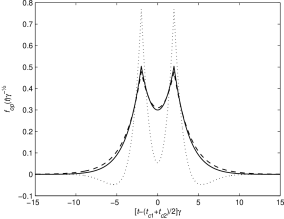
Figure 2: Optimized mode functions for $|t_{c2}-t_{c1}|\gamma=4$ and $\eta_{s}=1$. The three curves correspond to $\epsilon/\gamma=0$ (dashed line), $\epsilon/\gamma=0.08$ (solid line), and $\epsilon/\gamma=0.2$ (dotted line).

Figure 3 shows the optimized fidelity (solid lines) as a function of $\epsilon/\gamma$ for $t_{c1}=t_{c2}$ and the fidelity calculated from the optimal mode function at zero intensity (dashed curves). The solid and dashed curves are almost identical for small $\epsilon/\gamma$, so the optimal mode function at zero intensity is close to optimal in the region where the fidelity is high and hence provides an analytical approximation to the optimal choice of signal state mode function. The figure shows that the fidelity decreases when the intensity increases. This is as expected because a larger mean photon flux results in larger contributions from higher photon number states to the output state.

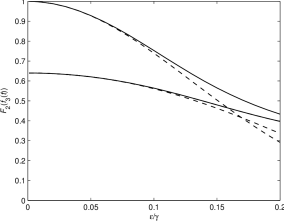
Figure 3: Fidelity for $t_{c1}=t_{c2}$ calculated using the optimized signal mode function (solid lines) and the optimal mode function at zero intensity (19) (dashed lines). Perfect signal detection $\eta_{s}=1$ is assumed for the curves approaching 1 to the left, while $\eta_{s}=0.8$ for the curves approaching 0.64.

The fidelity decreases when the temporal distance between the trigger detector clicks increases from zero as is apparent from figure 4, which shows the fidelity as a function of $|t_{c2}-t_{c1}|\gamma$. When the click distance is different from zero, the two photons no longer belong to precisely the same mode. We return to this point in section V, where we also obtain an analytical expression for the two-photon state fidelity as a function of click distance in the small intensity limit. The fidelity calculated from the optimal mode function at zero intensity (19) is also shown in figure 4 (the dashed curve), and it is seen that (19) is a good approximation to the optimal mode function even if the click distance is large (provided $\epsilon/\gamma$ is not too large).

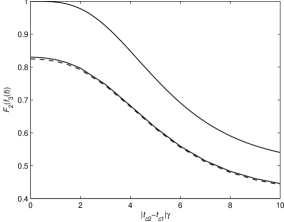
Figure 4: Fidelity as a function of temporal distance between the trigger detector clicks for $\epsilon/\gamma=0$ (upper solid line) and $\epsilon/\gamma=0.08$ (lower solid line) calculated using the optimized signal mode function. The dashed line shows the fidelity for $\epsilon/\gamma=0.08$ obtained from the mode function (19). Perfect signal detection $\eta_{s}=1$ is assumed.

We note that the generation method described here favors close click events since

$$\frac{\langle\hat{a}_{+}^{\dagger}(t_{c1})\hat{a}_{+}^{\dagger}(t_{c2})\hat{a}_{+}(t_{c2})\hat{a}_{+}(t_{c1})\rangle}{\langle\hat{a}_{+}^{\dagger}(t_{c1})\hat{a}_{+}(t_{c1})\rangle\langle\hat{a}_{+}^{\dagger}(t_{c2})\hat{a}_{+}(t_{c2})\rangle}=\\ 1+\left(\frac{\mathrm{e}^{-\mu|t_{c2}-t_{c1}|}}{2\mu}-\frac{\mathrm{e}^{-\lambda|t_{c2}-t_{c1}|}}{2\lambda}\right)^{2}\bigg{/}\left(\frac{1}{2\mu}-\frac{1}{2\lambda}\right)^{2}$$ (20)

increases from one to two when $|t_{c2}-t_{c1}|\gamma$ decreases from infinity to zero: the trigger events are bunched in time.

V Mode occupation description of the conditional state in the low intensity limit

In the previous sections we characterized the output state by the Wigner function $W_{click}$ from which we were able to calculate the fidelity for an arbitrary state in an arbitrary mode. However, a deeper understanding of the nature of the conditionally produced signal beam state can be obtained by considering the state as built up of photons occupying specific temporal modes. A detailed mode description of multi-photon states and manipulations of such states is given in Ref. rohde . In the present section we use this approach to investigate the state generated when conditioning on $n$ trigger detector click events. It is assumed throughout that $\epsilon/\gamma\ll 1$.

If the trigger detector clicks are far apart, we know from Ref. nm that the fidelity for a single photon in each of the $n$ modes

$$g_{i}(t)\equiv\sqrt{\frac{\gamma}{2}}\mathrm{e}^{-\frac{\gamma}{2}|t-t_{ci}|},\qquad i=1,2,\ldots,n$$ (21)

is unity. On the other hand, for $n=2$ and $t_{c1}=t_{c2}$ we found in the last section that the fidelity is unity for two photons in the mode $g_{1}(t)$. In both limits the state generated in the signal beam conditioned on two clicks is thus on the form $|\psi_{2}\rangle=N_{\psi_{2}}\iint dtdt^{\prime}g_{1}(t)g_{2}(t^{\prime})\hat{a}_{-}^{\dagger}(t)\hat{a}_{-}^{\dagger}(t^{\prime})|0\rangle$, where $N_{\psi_{2}}$ is a normalization constant. One is thereby led to consider whether this result is also valid for intermediate separation of the trigger detector clicks. In the appendix we show that the state generated in the signal beam when conditioning on $n$ trigger detector click events is

$$|\psi_{n}\rangle=N_{\psi_{n}}\left[\prod_{i=1}^{n}\int dt_{i}g_{i}(t_{i})\hat{a}_{-}^{\dagger}(t_{i})\right]|0\rangle,$$ (22)

where $N_{\psi_{n}}$ is a normalization constant.

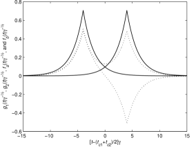
Figure 5: Mode functions $g_{1}(t)$ and $g_{2}(t)$ (solid lines) and $f_{a}(t)$ and $f_{b}(t)$ (dotted lines) for $(t_{c2}-t_{c1})\gamma=8$.

To illustrate the meaning of (22) we consider the case $n=2$ in some detail. Two orthogonal mode functions are constructed from $g_{1}(t)$ and $g_{2}(t)$:

$$f_{a}(t) = \frac{1}{\sqrt{2(1+I_{12})}}\left[g_{1}(t)+g_{2}(t)\right],$$ (23)

$$f_{b}(t) = \frac{1}{\sqrt{2(1-I_{12})}}\left[g_{1}(t)-g_{2}(t)\right],$$ (24)

where

$$I_{ij} \equiv \int g_{i}(t)g_{j}(t)dt$$ (25)

$$= \left(1+\frac{\gamma}{2}|t_{ci}-t_{cj}|\right)\exp\left(-\frac{\gamma}{2}|t_{ci}-t_{cj}|\right).$$

The four mode functions are illustrated in figure 5 for $\gamma(t_{c2}-t_{c1})=8$. Inserting (23) and (24) in (22) we obtain

$$|\psi_{2}\rangle=\frac{1+I_{12}}{\sqrt{2(1+I_{12}^{2})}}|2,0\rangle_{ab}-\frac{1-I_{12}}{\sqrt{2(1+I_{12}^{2})}}|0,2\rangle_{ab},$$ (26)

where $|x,y\rangle_{ab}=|x\rangle_{a}\otimes|y\rangle_{b}$ and $|x\rangle_{j}$ means $x$ photons in the mode $f_{j}(t)$. Figure 6 shows the norm square of the coefficients in (26). Since $f_{a}(t)$ is identical to the optimal mode function for $\epsilon/\gamma\ll 1$ (19), the upper curve shows the maximal two-photon state fidelity as a function of temporal distance between the conditioning clicks (i.e. the same curve as in figure 4). For small $\gamma|t_{c2}-t_{c1}|$ we find from equations (25) and (26) that

$$F_{2}(f_{a}(t))\simeq 1-\left(\frac{\gamma}{4}|t_{c2}-t_{c1}|\right)^{4}.$$ (27)

Hence we still have a good two-photon state even if the trigger detector clicks are not exactly simultaneous.

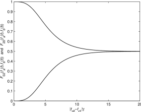
Figure 6: The upper (lower) curve shows the probability to detect two (zero) photons in the mode $f_{a}(t)$ and zero (two) photons in the mode $f_{b}(t)$ as a function of temporal distance between trigger detector clicks when $\epsilon/\gamma\rightarrow 0$.

The optimal mode function for a general $n$ is obtained by maximizing the fidelity between (22) and an $n$-photon state

$$|n\rangle_{f}=\frac{1}{\sqrt{n!}}\left[\int dtf(t)\hat{a}_{-}^{\dagger}(t)\right]^{n}|0\rangle,$$ (28)

where $f(t)$ is the mode function to be optimized. The $n$-photon state fidelity is

$$F_{n}(f(t))=|\langle\psi_{n}|n\rangle_{f}|^{2}=n!|N_{\psi_{n}}|^{2}\prod_{i=1}^{n}\left|\int f(t_{i})g_{i}(t_{i})dt_{i}\right|^{2}.$$ (29)

It is apparent that the phase of $f(t)$ should be time independent to maximize $F_{n}(f(t))$, and hence we choose $f(t)$ real. Variational optimization of $\prod_{i=1}^{n}\int f(t_{i})g_{i}(t_{i})dt_{i}$ leads to

$$\xi f(t)=\sum_{i=1}^{n}g_{i}(t)\prod_{\begin{subarray}{c}j=1\\ j\neq i\end{subarray}}^{n}\int f(t_{j})g_{j}(t_{j})dt_{j},$$ (30)

and thus

$$f(t)=\sum_{i=1}^{n}c_{i}g_{i}(t),$$ (31)

where the constants $c_{i}$ and $\xi$ are determined from the highly nonlinear set of equations

$$\xi c_{i}=\prod_{\begin{subarray}{c}j=1\\ j\neq i\end{subarray}}^{n}\sum_{k=1}^{n}c_{k}I_{kj}$$ (32)

and

$$1=\sum_{i=1}^{n}\sum_{j=1}^{n}c_{i}c_{j}I_{ij}.$$ (33)

For $n=2$ equations (32) and (33) are $\xi c_{1}=c_{1}I_{12}+c_{2}$, $\xi c_{2}=c_{1}+c_{2}I_{12}$, and $1=c_{1}^{2}+c_{2}^{2}+2c_{1}c_{2}I_{12}$, and hence $c_{1}=c_{2}=1/\sqrt{2(1+I_{12})}$ and $\xi=1+I_{12}$ in agreement with Eq. (19). For $n=3$ and $t_{c2}-t_{c1}=t_{c3}-t_{c2}$ we obtain

$$c_{1} = c_{3}=\sqrt{\frac{I_{12}^{2}-2(1+I_{13})+I_{12}\sqrt{I_{12}^{2}+4(1+I_{13})}}{6[2I_{12}^{2}-(1+I_{13})](1+I_{13})}},$$

$$c_{2} = -2c_{1}I_{12}+\sqrt{1+2c_{1}^{2}[2I_{12}^{2}-(1+I_{13})]},$$ (34)

and for $t_{c2}=t_{c1}$

$$c_{1} = c_{2}=\sqrt{\frac{(4-I_{13}^{2})-\sqrt{(4-I_{13}^{2})^{2}-16(1-I_{13}^{2})}}{24(1-I_{13}^{2})}},$$

$$c_{3} = \frac{1-6c_{1}^{2}}{3c_{1}I_{13}}.$$ (35)

The three-photon state fidelity for these special cases is shown as a function of click distance in figure 7. In the former case the fidelity decreases from unity to $3!/3^{3}$, when the click distance increases from zero to infinity, while in the latter case it decreases from unity to $3\cdot 2^{2}/3^{3}$, but in both cases a broad region with a fidelity close to unity exists.

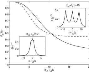
Figure 7: Three-photon state fidelity as a function of temporal distance between the first and the last trigger detector clicks for $t_{c3}-t_{c2}=t_{c2}-t_{c1}$ (solid line) and $t_{c1}=t_{c2}$ (dashed line). The insets show the optimal mode function $f(t)$ for the former case for $|t_{c3}-t_{c1}|\gamma=3$ (left) and $|t_{c3}-t_{c1}|\gamma=15$ (right). $\epsilon/\gamma\ll 1$ is assumed.

VI Conclusion

In conclusion we presented a theoretical description of conditional higher photon number state generation from a continuous-wave light source. We calculated the Wigner function for the output state conditioned on two trigger detector clicks and determined its overlap with a two-photon state. The output state mode function that gives rise to the largest overlap was found. In the low intensity limit, we showed that the state generated in the signal beam when conditioning on $n$ trigger detector click events is $|\psi_{n}\rangle=N_{\psi_{n}}\left[\prod_{i=1}^{n}\int dt_{i}g_{i}(t_{i})\hat{a}_{-}^{\dagger}(t_{i})\right]|0\rangle$, where $g_{i}(t)$ is a function localized around the time for the $i$th click. From this we obtain the optimal mode function and fidelity for $n$-photon state generation at low intensity. For small temporal distance between the trigger detector clicks and $n=2$ the optimized fidelity is unity minus a small correction of fourth order in the temporal click distance.

In the present treatment we averaged over all possible trigger detector outcomes outside the small time windows specified by the trigger mode functions, but for finite intensities larger fidelities are obtained if we condition on dark intervals between the $n$ clicks (see nm ).

Appendix A Conditional signal beam state at low intensity

In this appendix we prove that the state generated in the signal beam when conditioning on $n$ trigger detector clicks at times $t_{c1},\ldots,t_{cn}$ is given by (22) in the limit $\epsilon/\gamma\rightarrow 0$. Since the normally ordered moments determine the phase space P function lee , it is sufficient to prove that the expectation value obtained from (22) of all normally ordered products of signal beam field operators is equal to the expectation value obtained from the two-time correlation functions (11), when conditioning on the trigger detector clicks, i.e.

$$\lim_{\epsilon\rightarrow 0}\bigg{\{}\Big{\langle}\Big{[}\prod_{i=1}^{n}\hat{a}_{+}^{\dagger}(t_{ci})\Big{]}\Big{[}\prod_{j=1}^{m}\hat{a}_{-}^{\dagger}(t^{\prime}_{j})\Big{]}\Big{[}\prod_{k=1}^{p}\hat{a}_{-}(t^{\prime\prime}_{k})\Big{]}\\ \Big{[}\prod_{q=1}^{n}\hat{a}_{+}(t_{cq})\Big{]}\Big{\rangle}\Big{/}\Big{\langle}\Big{[}\prod_{i=1}^{n}\hat{a}_{+}^{\dagger}(t_{ci})\Big{]}\Big{[}\prod_{q=1}^{n}\hat{a}_{+}(t_{cq})\Big{]}\Big{\rangle}\bigg{\}}=\\ \int\Big{[}\prod_{i=1}^{n}g_{i}(t_{i})\Big{]}\Big{[}\prod_{q=1}^{n}g_{q}(t_{n+q})\Big{]}\langle 0|\Big{[}\prod_{i=1}^{n}\hat{a}_{-}(t_{i})\Big{]}\\ \Big{[}\prod_{j=1}^{m}\hat{a}_{-}^{\dagger}(t^{\prime}_{j})\Big{]}\Big{[}\prod_{k=1}^{p}\hat{a}_{-}(t^{\prime\prime}_{k})\Big{]}\Big{[}\prod_{q=1}^{n}\hat{a}^{\dagger}_{-}(t_{n+q})\Big{]}|0\rangle\\ \Big{(}\prod_{i=1}^{2n}dt_{i}\Big{)}\Big{/}\int\Big{[}\prod_{i=1}^{n}g_{i}(t_{i})\Big{]}\Big{[}\prod_{q=1}^{n}g_{q}(t_{n+q})\Big{]}\\ \langle 0|\Big{[}\prod_{i=1}^{n}\hat{a}_{-}(t_{i})\Big{]}\Big{[}\prod_{q=1}^{n}\hat{a}^{\dagger}_{-}(t_{n+q})\Big{]}|0\rangle\Big{(}\prod_{i=1}^{2n}dt_{i}\Big{)}$$ (36)

The left hand side is evaluated using Wick’s theorem for Gaussian states with zero means louisell , which states that

$$\langle\hat{A}_{1}\hat{A}_{2}\ldots\hat{A}_{2k}\rangle=\langle\hat{A}_{1}\hat{A}_{2}\rangle\langle\hat{A}_{3}\hat{A}_{4}\hat{A}_{5}\ldots\hat{A}_{2k}\rangle\\ +\langle\hat{A}_{1}\hat{A}_{3}\rangle\langle\hat{A}_{2}\hat{A}_{4}\hat{A}_{5}\ldots\hat{A}_{2k}\rangle+\ldots\\ +\langle\hat{A}_{1}\hat{A}_{2k}\rangle\langle\hat{A}_{2}\hat{A}_{3}\hat{A}_{4}\ldots\hat{A}_{2k-1}\rangle,$$ (37)

while $\langle\hat{A}_{1}\hat{A}_{2}\ldots\hat{A}_{2k+1}\rangle=0$, where $\hat{A}_{i}$ is either an annihilation or a creation operator and $k$ is a positive integer. The left hand side may thus be expressed in terms of $\langle\hat{a}^{\dagger}_{\pm}(t)\hat{a}_{\pm}(t^{\prime})\rangle$ and $\langle\hat{a}_{\pm}(t)\hat{a}_{\mp}(t^{\prime})\rangle$. For small $\epsilon/\gamma$

$$\langle\hat{a}^{\dagger}_{\pm}(t)\hat{a}_{\pm}(t^{\prime})\rangle = \frac{2\epsilon^{2}}{\gamma}\left(1+\frac{\gamma}{2}|t-t^{\prime}|\right)\mathrm{e}^{-\frac{\gamma}{2}|t-t^{\prime}|},$$ (38)

$$\langle\hat{a}_{\pm}(t)\hat{a}_{\mp}(t^{\prime})\rangle = \sqrt{\frac{2\epsilon^{2}}{\gamma}}\sqrt{\frac{\gamma}{2}}\mathrm{e}^{-\frac{\gamma}{2}|t-t^{\prime}|}.$$ (39)

It follows that the left hand side of (36) is zero if $m\neq p$, since in that case we have to combine operators, where the expectation value of the product of the operators is zero. It also follows that the denominator on the left hand side of (36) is proportional to $\epsilon^{2n}$. In the numerator the lowest order terms in $\epsilon$ are obtained by combining as many $\hat{a}^{\dagger}_{-}$ operators as possible with $\hat{a}^{\dagger}_{+}$ operators and as many $\hat{a}_{-}$ operators as possible with $\hat{a}_{+}$ operators. These terms are proportional to $\epsilon^{\max(2n,2m)}$ for $m=p$. To obtain a nonzero left hand side in the limit $\epsilon/\gamma\rightarrow 0$, it is thus necessary to require that $m=p\leq n$. It is immediately apparent that the right hand side of (36) is zero if $m=p\leq n$ is not satisfied.

We now consider the case $m=p\leq n$ and by combining the operators as described above and using (39) and (38) and the definitions (21) and (25) we obtain for the lowest order terms of the left hand side (LHS) of (36)

$$\mathrm{LHS}=\frac{1}{(n-m)!}\sum_{P_{i}}\sum_{P_{j}}g_{i_{1}}(t^{\prime}_{1})\ldots g_{i_{m}}(t^{\prime}_{m})g_{j_{1}}(t^{\prime\prime}_{1})\ldots\\ g_{j_{m}}(t^{\prime\prime}_{m})I_{i_{m+1},j_{m+1}}\ldots I_{i_{n},j_{n}}\Big{/}\sum_{P_{j}}I_{1,j_{1}}\ldots I_{n,j_{n}},$$ (40)

where the summations are over all permutations of the $n$ $i$-indices and all permutations of the $n$ $j$-indices, respectively. The right hand side of (36) is evaluated using the relation

$$\hat{a}_{-}(t^{\prime\prime}_{k})\left[\prod_{i=1}^{n}\hat{a}_{-}^{\dagger}(t_{i})\right]|0\rangle=\\ \sum_{j=1}^{n}\delta(t^{\prime\prime}_{k}-t_{j})\left[\prod_{\begin{subarray}{c}i=1\\ i\neq j\end{subarray}}^{n}\hat{a}_{-}^{\dagger}(t_{i})\right]|0\rangle$$ (41)

repeatedly, which leads to

$$\langle 0|\prod_{i=1}^{n}\hat{a}_{-}(t_{i})\prod_{j=1}^{m}\hat{a}_{-}^{\dagger}(t^{\prime}_{j})\prod_{k=1}^{m}\hat{a}_{-}(t^{\prime\prime}_{k})\prod_{q=1}^{n}\hat{a}^{\dagger}_{-}(t_{n+q})|0\rangle=\\ \frac{1}{(n-m)!}\sum_{P_{i}}\sum_{P_{j}}\delta(t^{\prime}_{1}-t_{i_{1}})\ldots\delta(t^{\prime}_{m}-t_{i_{m}})\\ \delta(t^{\prime\prime}_{1}-t_{n+j_{1}})\ldots\delta(t^{\prime\prime}_{m}-t_{n+j_{m}})\delta(t_{i_{m+1}}-t_{n+j_{m+1}})\\ \ldots\delta(t_{i_{n}}-t_{n+j_{n}}).$$ (42)

Inserting (42) in (36) we immediately obtain the result (40) for the right hand side of (36).

References

(1) B. T. H. Varcoe, S. Brattke, M. Weidinger, and H. Walther
Nature (London) 403, 743 (2000).
(2) P. Bertet, S. Osnaghi, P. Milman, A. Auffeves,
P. Maioli, M. Brune, J. M. Raimond, and S. Haroche
Phys. Rev. Lett. 88, 143601 (2002).
(3) S. Gleyzes, S. Kuhr, C. Guerlin, J. Bernu,
S. Deléglise, U. B. Hoff, M. Brune, J.-M. Raimond, and S. Haroche,
quant-ph/0612031.
(4) C. Brunel, B. Lounis, P. Tamarat, and M. Orrit,
Phys. Rev. Lett. 83, 2722 (1999).
(5) P. Grangier, A. L. Levenson and J. P. Poizat,
Nature (London) 396, 537 (1998).
(6) S. R. Friberg, S. Machida and Y. Yamamoto,
Phys. Rev. Lett. 69, 3165 (1992).
(7) M. Oxborrow and A. G. Sinclair, Contemp.
Phys. 46, 173 (2005).
(8) A. Ourjoumtsev, R. Tualle-Brouri, and P. Grangier,
Phys. Rev. Lett. 96, 213601 (2006).
(9) M. Dakna, T. Anhut, T. Opatrný, L. Knöll, and
D.-G. Welsch, Phys. Rev. A 55, 3184 (1997).
(10) M. S. Kim, E. Park, P. L. Knight, and H. Jeong, Phys.
Rev. A 71, 043805 (2005).
(11) J. Fiurasek, R. Garcia-Patron, and N. J. Cerf,
Phys. Rev. A 72, 033822 (2005).
(12) A. Ourjoumtsev, R. Tualle-Brouri, J.
Laurat, and P. Grangier, Science 312, 83 (2006).
(13) J. S. Neergaard-Nielsen, B. M. Nielsen, C. Hettich, K. Mølmer,
and E. S. Polzik, Phys. Rev. Lett. 97, 083604 (2006).
(14) K. Wakui, H. Takahashi, A. Furusawa, and M. Sasaki,
quant-ph/0609153.
(15) M. Sasaki and S. Suzuki, Phys. Rev. A 73,
043807 (2006).
(16) K. Mølmer, Phys. Rev. A 73, 063804 (2006).
(17) A. E. B. Nielsen and K. Mølmer, Phys. Rev. A 75,
023806 (2007).
(18) M. Ban, J. Opt. B: Quantum Semiclass. Opt. 1 (1999)
L9-L11.
(19) P. D. Drummond and M. D. Reid, Phys. Rev. A
41, 3930 (1990).
(20) P. P. Rohde, W. Mauerer, and C. Silberhorn, quant-ph/0609004.
(21) C. T. Lee, Phys. Rev. A 45, 6586 (1992).
(22) W. H. Louisell, 1973, Quantum Statistical
Proporties of Radiation. Wiley, New York, 1973.